R E S E A R C H
Open Access
Hierarchical complexity control algorithm
for HEVC based on coding unit depth
decision
Fen Chen, Peng Wen, Zongju Peng
*, Gangyi Jiang, Mei Yu and Hua Chen
Abstract
The next-generation High Efficiency Video Coding (HEVC) standard reduces the bit rate by 44% on average compared to the previous-generation H.264 standard, resulting in higher encoding complexity. To achieve normal video coding in power-constrained devices and minimize the rate distortion degradation, this paper proposes a hierarchical complexity control algorithm for HEVC on the basis of the coding unit depth decision. First, according to the target complexity and the constantly updated reference time, the coding complexity of the group of pictures layer and the frame layer is allocated and controlled. Second, the maximal depth is adaptively assigned to the coding tree unit (CTU) on the basis of the correlation between the residual information and the optimal depth by establishing the complexity-depth model. Then, the coding unit smoothness decision and adaptive low bit threshold decision are proposed to constrain the unnecessary traversal process within the maximal depth assigned by the CTU. Finally, adaptive upper bit threshold decision is used to continue the necessary traversal process at a larger depth than the maximal depth of allocation to guarantee the quality of important coding units. Experimental results show that our algorithm can reduce the encoding time by up to 50%, with notable control precision and limited performance degradation. Compared to state-of-the-art algorithms, the proposed algorithm can achieve higher control accuracy.
Keywords:Complexity control, High Efficiency Video Coding, Maximal coding depth, Rate distortion optimization
1 Introduction
With the development of capture and display technologies, high-definition video is being widely adopted in many fields, such as television, movies, and education. To effi-ciently store and transmit large amounts of high-definition video data, the Joint Collaborative Team on Video Coding (JCT-VC), consisting of ISO-IEC/MPEG and ITU-T/ VCEG, proposed High Efficiency Video Coding (HEVC) [1] as the next-generation international video coding standard in 2013. Compared with the previous-generation video cod-ing standard H.264/AVC [2], HEVC uses new technologies, such as the quad-tree encoding structure [3], which reduces the average bit rate by 44% while providing the same ob-jective quality [4]. However, the computational complexity of HEVC is high [5], and HEVC cannot be implemented on all devices, especially mobile multimedia devices with lim-ited power capacity. To reduce the computational
complexity of HEVC, many algorithms have been proposed to speed up the motion estimation [6], mode decision [7], and coding unit (CU) splitting [8]. However, the speedup performance is obtained at the cost of the degradation of rate distortion performance. In addition, the computational complexity reduction of these algorithms is not consistent for different video sequences. Hence, it is significant to con-trol the coding complexity for different multimedia devices and sequences.
The research goals of HEVC complexity control are high control accuracy and rate distortion performance. High control accuracy can minimize the loss of rate dis-tortion performance. Many researchers have devoted considerable efforts toward achieving these goals. Correa et al. used the spatial-temporal correlation of the coding tree unit (CTU) to limit the maximal depth of restricted CTUs. Thus, they reduced the coding complexity by 50% while incurring a small degradation in the rate dis-tortion performance [9]. Correa et al. further limit the max-imal depth of CTU in restricted frames to achieve * Correspondence:[email protected]
Faculty of Information Science and Engineering, Ningbo University, Ningbo, China
complexity control [10]. The abovementioned algorithms [9,10] do not fully consider the image characteristics when determining the restricted CTUs and frames. Correa et al. used the CTU rate distortion cost in the previous frame as the basis for determining whether the current CTU should be constrained or unconstrained, and they controlled the coding complexity by limiting the modes and the maximal depth [11]. Furthermore, by adjusting the configuration of the coding parameters, they were able to restrict the target complexity to 20% [12]. However, the relationship between the coding parameters and the complexity is obtained off-line and cannot adapt to video with different features. Deng et al. employed the visual perception factor to limit the maximal depth in order to realize complexity allocation [13]. Further, they studied the relationship between the maximal depth and the complexity and limited the max-imal CTU depth by combining the temporal correlation and visual weight. Their algorithm not only controls the computational complexity but also guarantees the subject-ive and objectsubject-ive quality [14]. In addition, they have
proposed a complexity control algorithm for video encing, which is adaptable to the features of video confer-encing [15]. The abovementioned methods of complexity allocation [13–15] are more effective for sequences with less texture, while they result in degradation of the rate dis-tortion performance for sequences with rich texture. Zhang et al. established a statistical model to estimate the com-plexity of CTU coding and restricted the CTU depth tra-versal range to achieve complexity control. However, it cannot achieve accurate complexity control for the videos with large scene changes [16]. Amaya et al. proposed a complexity control method based on fast CU decisions [17]. They obtained thresholds for early termination at dif-ferent depths via online training. These thresholds are used to terminate the recursive CU process in advance. Their al-gorithm can restrict the target complexity to 60% while guaranteeing the coding performance. However, the control accuracy requires improvement and the rate distortion performance undergoes severe degradation as the target computational complexity decreases.
a
b
To further improve the control accuracy and reduce the rate distortion performance degradation, this paper proposes a hierarchical complexity control algorithm based on the CU depth decision. First, according to the target complexity and the constantly updated reference time, the coding complexity of the group of pictures (GOP) layer and frame layer is assigned and controlled. Second, the complexity weight of the current CTU is calculated, and the maximal depth is adaptively allocated according to the encoding complexity-depth model (ECDM) and the video encoding feature. Finally, the rate distortion optimization (RDO) process is terminated early or continued on the basis of the CU smoothness decision and the adaptive upper and low bit threshold decision. This paper has two main contributions: (1) We propose a method with period-ical updating strategy to predict the reference time. (2) We propose two kinds of adaptive complexity reduction methods, which adapt to different video contents well.
The remainder of this paper is organized as follows. Section 2describes the quad-tree structure and the rate distortion optimization process of HEVC. Section3 pro-vides a detailed explanation of the proposed method.
Section 4 presents and discusses the experimental
results. Finally, Section5concludes the paper.
2 Quad-tree structure and rate distortion optimization process of HEVC
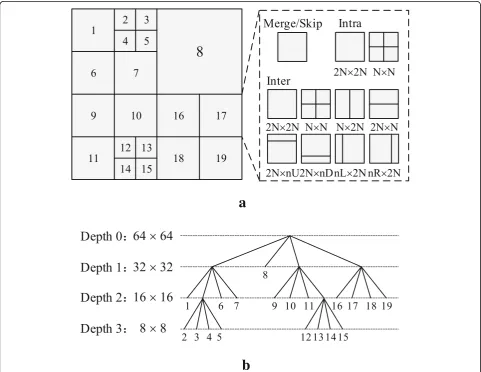
HEVC divides each frame into several CTUs of equal size. If the video is sampled according to the 4:2:0 sampling format, then each CTU contains a luma and two chroma coding tree blocks, which form the root of the quad-tree structure. As shown in Fig.1a, CTU can be divided into several equal-sized CUs according to the quad-tree struc-ture, which ranges in size from 8 × 8 to 64 × 64. The CU is the basic unit of intra or inter prediction. Each CU can be divided into 1, 2, or 4 prediction units (PUs), and each PU is a region that uses the same prediction. HEVC supports 11 candidate PU splitting modes, Merge/Skip mode, two intra modes (2N × 2N, N × N), and eight inter modes (2N × 2N, N × N, N × 2N, 2N × N, 2N × nU, 2N × nD, nL × 2N, nR × 2N). The transform unit (TU) is a shared trans-form and quantization square region defined by a quad-tree partitioning of a leaf CU. Each PU contains luma and chroma prediction blocks (PBs) and the corre-sponding syntax elements. The size of a PB can range from 4 × 4 to 64 × 64. Each TU contains luma and chroma transform blocks (TBs) and the corresponding syntax ele-ments. The size of a TB can range from 4 × 4 to 32 × 32.
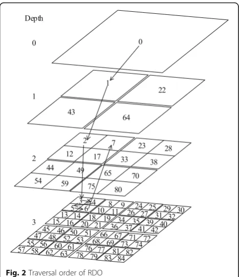
RDO process of the quad-tree structure is used to deter-mine the optimal partition of the CTU. RDO needs to traverse entire depth in the order shown in Fig.2with all the PU splitting modes. By comparing the minimal rate distor-tion cost of the parent CU and the sum of the minimal rate distortion costs of four sub CUs, it is determined whether
the parent CU should be divided into four sub CUs. If the minimal rate distortion cost of the parent CU is smaller, then partitioning is not performed; otherwise, it is performed.
Analysis of the HEVC quad-tree structure and RDO process shows that the high computational complexity of HEVC is mainly caused by the depth traversal with the various modes. Considering the limited computational power of multimedia devices, we design a complexity control algorithm that skips the unnecessary CU depth and performs early termination of the mode search ac-cording to the video coding feature.
3 Methods
This paper proposes a hierarchical complexity control algorithm based on the coding unit depth decision, as shown in Fig. 3. The proposed algorithm includes the complexity allocation and control of GOP layer and frame layer, the CTU complexity allocation (CCA), the
Fig. 2Traversal order of RDO
CU smoothness decision (CSD) method, and the adap-tive upper and lower bit threshold decision (ABD) method. The CCA divides the complexity weight of the CTU and allocates the maximal depth to the CTU in combination with the ECDM model. The CSD and ABD further restrict the RDO process and reduce the compu-tational complexity.
3.1 Complexity allocation and control of GOP layer and frame layer
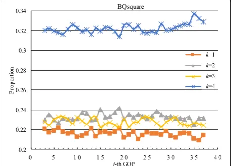
Among the encoding process, the first GOP has only one I frame, and is different from other GOPs. In the second GOP, the number of reference frames in the first three frames is less than that in other frames. Except the first two GOPs, the encoding structures of the subse-quent GOPs are similar, and the encoding time is nearly consistent. Moreover, a GOP except the first GOP con-tainsGframes, and for convenience of presentation, we refer to the m-th frame (m= 1,2,3, …, G) in the j-th GOP as frame (m,j). For certaink, the frames (k, j) are corresponding frames. The encoding parameters of the corresponding frames in consecutive GOPs are consist-ent. Hence, their proportion of the encoding time is similar. Figure 4 shows the proportion of the encoding time in different GOPs for the BQsquaresequence. The encoding time proportionρ(k,j) is calculated as:
ρðk;jÞ ¼ t kð ;jÞ
XG
m¼1
t mð ;jÞ
; ð1Þ
wheret(k,j) is the coding time of frame (k,j). Clearly, the
ρ(k,j) is nearly consistent for certain k. For example,
ρ(4,j) slightly varies in a small range from 0.314 to 0.337. Inspired by the phenomena, we can estimate the refer-ence coding time of entire sequrefer-enceTo by normal
cod-ing some frames.Tois the predicted value of the normal
coding time of entire sequence, and normal coding means that frames should be encoded without complex-ity control.
The first three GOPs are normally coded to obtain the initial To, and after the third GOP, a frame is normally
coded for every four GOPs to updateTo, i.e.,
To ¼
J−3
ð Þ X2G f¼Gþ1
tfþ
X2G
f¼0
tf; if f ¼2G
1 f−2G
ð Þ=ð4GÞ þ1 X
f−2G
ð Þ=ð4GÞ
g¼0
tg4Gþ2G
ρðG;3Þ
ðJ−3Þ þX 2G
f¼0
tf ; if ðf−2GÞ%ð4GÞ ¼0
8 > > > > > > > > > > > > < > > > > > > > > > > > > : ;
ð2Þ
wherefdenotes thef-th frame,f∈[0,F−1],J is the total number of GOPs to be encoded, and tfdenotes the ac-tual coding time of the f-th frame. Constantly updating Tocauses it to further approach its true value.
After encoding the (j−1)-th GOP, the target coding time of the j-th GOP TGOPj is determined according to the remaining target time and the number of remaining frames to be coded. It is calculated as
TGOPj ¼TcTo−Tcoded F−Fcoded
G; ð3Þ
where Tc is the target complexity proportion, Tc⋅To is
the target coding time of entire sequence,Tcoded is the
consumed encoding time,Fcoded is the number of coded
frames, and F is the total number of frames to be encoded.
In the case of complexity control algorithms, the rate distortion performance of video sequences severely dete-riorates as the target encoding time decreases [9–15]. Moreover, the coding time of each frame in one GOP differs significantly because of different coding parame-ters. Hence, the time proportion rather than absolute time is reasonably used to regulate the encoding com-plexity. In the study, to achieve temporal-consistent rate distortion performance, the proportion of time saving is the same in one GOP. To maintain the same proportion of the time saving for each frame in the GOP, we allo-cate the target encoding time by using the temporal sta-bility of the encoding proportion in the frame layer.
For complexity control of the frame layer, it is import-ant to maintain good rate distortion performance. In the proposed algorithm, we estimate the actual time saving of the coded frame by considering the difference be-tween the normal coding time of the coded frame and the actual coding time. Then, the following strategies are adopted. (1) If the sum of the actual time saving of
already coded frames is greater than the target time saving of the entire sequence, normal coding is carried out in time to avoid degradation of the rate distortion perform-ance. (2) When the sum of actual time saving of the coded frames is less than the target time saving of the entire se-quence, the remaining frames still need to be encoded under control. (3) When the actual time saving of the pre-vious frame is much greater than the target time saving of the previous frame, the degree of control of the current frame needs to be reduced. Therefore, the current frame only uses the CSD method to save the coding time and achieve better rate distortion performance.
3.2 CTU complexity allocation
The proportion of the CU at each depth changes according to the characteristics and coding parameters of video se-quences. Based on the residual information and the ECDM model, a complexity allocation method for the CTU layer is proposed in this study. The target complexity of the frame layer is reasonably allocated to each CTU by avoiding the RDO process in the unnecessary CU depth.
3.2.1 Complexity weight calculation
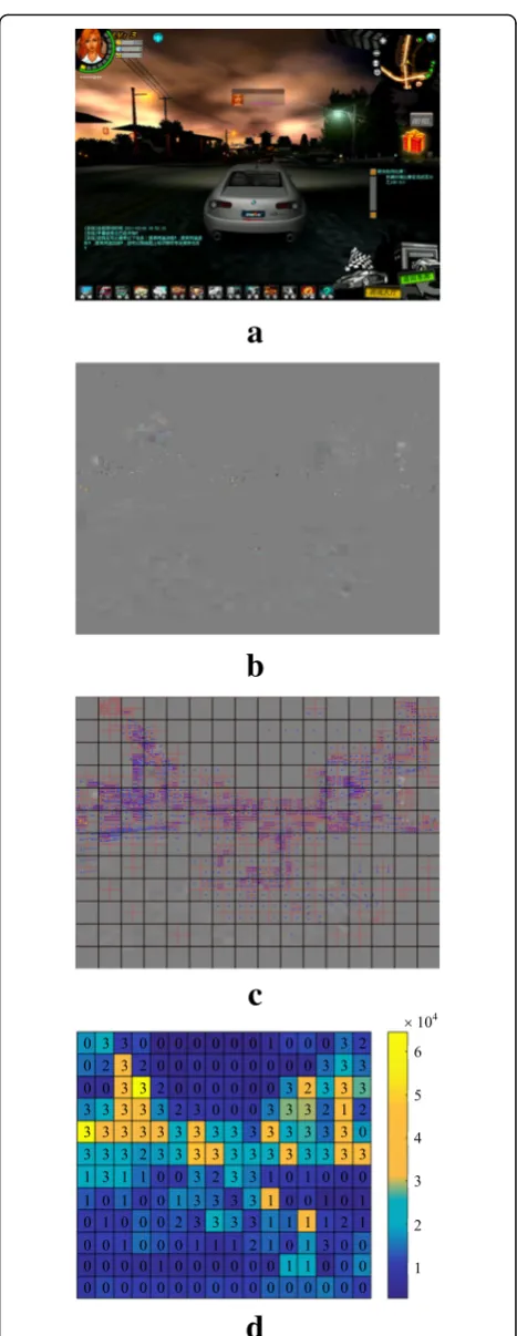
In the low-delay configuration of HEVC, the CTU encoded with large depth often corresponds to the region with strong motion or rich texture. Figure 5a shows the 16th
frame in sequence ChinaSpeed. Figure 5b shows the
residual of the ChinaSpeed. Figure 5c shows the optimal partition of ChinaSpeed and blue solid line indicates motion vector of CU. Clearly, the residual in motion regions is more obvious and the corresponding optimal partition is more precise. Therefore, when the CU depth is 0, the residual is reflected by the absolute difference between the original pixel and the predicted pixel. The mean absolute difference (MAD) of the CU is used as the basis for judging the pixel level fluctuation, and the abso-lute difference that is greater than the MAD is accumu-lated to obtain the effective sum of absolute differences (ESAD). Figure5d shows the relation between the ESAD and optimal depth of CTU. Here, the optimal depth refers to the depth calculated through the RDO process. The digit in each CTU represents the optimal depth, and color de-notes different ESAD. Clearly, the optimal depth is strongly related to the ESAD. Therefore, in the proposed algorithm, ESAD of thei-th CTU, denoted byωi, is used as the
com-plexity allocation weight of thei-th CTU.
3.2.2 Encoding complexity-depth model
Statistical analysis of the average coding complexity under the different maximal depthdmaxwas conducted to explore
the relationship between the coding complexity and dmax
of the CTU. We trained five sequences, as shown in Table1, on HM 13.0 software under the low delay P main configuration. Four different quantization parameter (QP)
a
b
d
c
values (i.e., 22, 27, 32, 37) are used. The coding time Cnð
dnmaxÞis obtained statistically whendnmaxis 0, 1, 2, and 3, re-spectively, in then-th CTU. The coding time whendnmax is 3 is regarded as the reference time, and the coding time is normalized whendnmaxis 0, 1, 2, and 3, respectively, i.e.,
CnðdnmaxÞ ¼
CnðdnmaxÞ
Cnð3Þ ;
dnmax∈f0;1;2;3g: ð4Þ
The normalized coding times whendmaxis 0, 1, 2, and
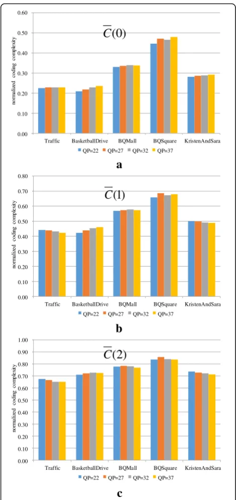
3, respectively, are summed and the average normalized coding timeCðdmaxÞis obtained. Figure6shows
normal-ized coding complexity difference of four QPs with dif-ferent maximal depth. We find that the difference of normalized encoding complexity with different QPs is small. Thus, we get mean of the training results of four QPs, as presented in Table1.
From mean of the training results, the average coding complexity TCTU under different dmax is obtained, and
the ECDM is established as follows:
TCTU ¼
1; dmax ¼3 0:75; dmax¼2 0:52; dmax¼1 0:31; dmax¼0 8 > > < > >
: ; ð5Þ
whereTCTU represents the average coding complexity of the CTU under differentdmax.
The CCA method is summarized as follows:
1) Obtain the target coding time Ttf andωiof thef-th
frame.
2) According to the allocation time of Tt
f and ωi, the
target coding time of thei-th CTUTiCTUis calculated as:
TiCTU ¼T t f−Rcoded XI
m¼i
ωm
ωi; ð6Þ
where Rcoded represents the sum of the actual coding
times of the all the coded CTUs in the current frame,
ωm represents the complexity allocation weight of the
m-th CTU in the corresponding frame of the last GOP, andIrepresents the number of CTUs in one frame.
4) Use the normal coding time of the CTU in the corresponding frame in the third GOP as the
normal-ized denominator to normalize TiCTU in order to
obtain the normalized target coding complexity of CTU T~iCTU.
Table 1Mean normalized coding complexity of four QPs at different maximal depths
Training sequence Cð0Þ Cð1Þ Cð2Þ
Traffic 0.23 0.43 0.66
BasketballDrive 0.22 0.44 0.72
BQMall 0.34 0.57 0.78
BQSquare 0.47 0.67 0.84
KristenAndSara 0.29 0.50 0.73
Average 0.31 0.52 0.75
0.00 0.10 0.20 0.30 0.40 0.50 0.60
Traffic BasketballDrive BQMall BQSquare KristenAndSara
no rm al iz ed c odi ng com p le xi ty
QP=22 QP=27 QP=32 QP=37
(0)
C
0.00 0.10 0.20 0.30 0.40 0.50 0.60 0.70 0.80Traffic BasketballDrive BQMall BQSquare KristenAndSara
no rm al iz ed codi ng com p le xi ty
QP=22 QP=27 QP=32 QP=37
(1)
C
0.00 0.10 0.20 0.30 0.40 0.50 0.60 0.70 0.80 0.90 1.00Traffic BasketballDrive BQMall BQSquare KristenAndSara
no rm al iz ed c o d ing co m p le xi ty
QP=22 QP=27 QP=32 QP=37
(2)
C
a
b
c
5) According to the ECDM andT~iCTU, set the maximal depth of the current CTU as:
dimax¼
0; if T~iCTU≤0:31 1; if 0:31<T~iCTU≤0:52 2; if 0:52<T~i
CTU≤0:75 3; if 0:75<T~iCTU≤1 8
> > > > < > > > > :
ð7Þ
In the proposed method, the frames in the first three GOPs are normally coded. Subsequently, only one frame out of every four GOPs is normally coded to updateT0and
ratio of CTU optimal depth is 0. When the motion is strong or the texture is rich, the maximal CTU depth deter-mined by Eq. (7) will degrade the rate distortion perform-ance. When the ratio is less than 0.4, the CU at depth 0 only tests Merge/Skip and inter 2N × 2N mode, and longer coding time is required for traversal of larger depths. Thus, Eq. (7) becomes:
dimax¼
1; if T~iCTU≤0:31 2; if 0:31<T~iCTU≤0:75 3; if 0:75<T~i
CTU≤1 8
> < >
: ð8Þ
3.3 CU smoothness decision
The CCA method avoids traversal of some unnecessary depths, but after allocating dmax, redundant traversal
may still occur for CUs with depth d∈[0,dmax]. It has
been observed that when the residual volatility is smooth and the motion is weak, the CU is more likely to be op-timal partition, as shown in Fig. 5c. Therefore, the current CU no longer proceeds with the deeper RDO process when the following conditions are satisfied: (1) the absolute difference between the original value and the predicted value of any pixel in the CU is smaller than a certain threshold, and (2) the motion vector is 0.
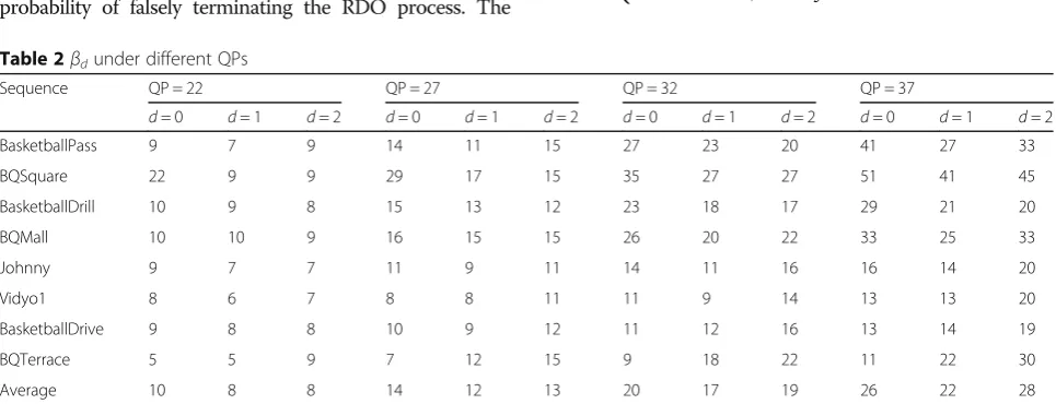
Apparently, the greater the threshold, the greater is the probability of falsely terminating the RDO process. The
threshold should be set on the basis of a tradeoff between the rate distortion performance and the computational complexity. To obtain the threshold, we perform explora-tive experiments by normal coding 150 frames under the low-delay configuration. The training sequences, as shown in Table2, with different features are encoded under QP = 22, 27, 32, and 37. We can obtain the partitioned quad-tree of all the CTUs. Further, we can directly obtain the number of CUs that is not optimal partition, statistically analyze them, and ensure that the former conditions with the threshold (ranging from 1 to 128) are satisfied. Hence, we can set a reasonable threshold by considering the rate dis-tortion performance and encoding speed. On the one hand, we constrain the false termination ratio within 1% by adjusting the threshold in order to achieve better rate dis-tortion performance. On the other hand, we should maximize the threshold to save more time. Hence, in the proposed method, the reasonable threshold βd at depth
leveldis given by:
βd¼ maxð Þχ s:t:
Eχd
Hd<0:01; χ∈1::128 ½ ; ; d¼0;1;2
ð9Þ
whereHdis the number of CUs at depth leveldthat is not optimal partition, and Eβd is the number of CUs at depth level d that is not optimally partitioned and satisfy the former conditions with β (β=1,2,3,…, 128). The βd
values for different training sequences under different QP are listed in Table2.
According to the average value, we obtain the thresh-old by Gaussian fitting:
β¼
49:88e−ðQ32−62:07:85Þ 2
; if d¼0 30:34e−ðQ25−51:42:4Þ
2
; if d¼1 181e−ðQ38−88:04:99Þ
2
; if d¼2 8
> > < > >
: ð10Þ
Table 2βdunder different QPs
Sequence QP = 22 QP = 27 QP = 32 QP = 37
d= 0 d= 1 d= 2 d= 0 d= 1 d= 2 d= 0 d= 1 d= 2 d= 0 d= 1 d= 2
BasketballPass 9 7 9 14 11 15 27 23 20 41 27 33
BQSquare 22 9 9 29 17 15 35 27 27 51 41 45
BasketballDrill 10 9 8 15 13 12 23 18 17 29 21 20
BQMall 10 10 9 16 15 15 26 20 22 33 25 33
Johnny 9 7 7 11 9 11 14 11 16 16 14 20
Vidyo1 8 6 7 8 8 11 11 9 14 13 13 20
BasketballDrive 9 8 8 10 9 12 11 12 16 13 14 19
BQTerrace 5 5 9 7 12 15 9 18 22 11 22 30
where Q is QP value of current sequence and β is the threshold under differentdasQchanges.
According to statistical analysis of the optimal CU mode that satisfies the abovementioned condition, the probability of the optimal mode being inter 2N × 2N is not less than 93.5%. Hence, after testing the inter 2N × 2N mode, the current CU is judged. If the con-dition is satisfied, then the traversal of the remaining modes and the RDO process are terminated.
The CSD method is summarized as follows:
1) Test the inter 2N × 2N mode and obtain the absolute difference between the original pixel value and the predicted pixel value of the current CU as well as the motion vector information.
2) Obtainβfrom the current CU depth and QP value.
3) If the absolute difference between the original value and the predicted value of any pixel in the CU is less thanβ, and the motion vector is 0, then the traversal of the remaining modes and the RDO process are terminated.
3.4 Adaptive upper and lower bit threshold decision On the one hand, due to the strict conditions of the CSD method, the time saving cannot reach to the target time. On the other hand, in the CCA method, the CU depth decision will lead to rate distortion performance degradation. Hence, we should further regulate the computational complexity on the basis of the CSD and CCA methods.
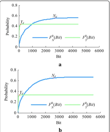
In [14], it has been shown that the greater the cor-responding bit of the current CU, the greater is the probability that it is not optimal partition. For further analyzing the relationship between bit of the current CU and the probability that it is not optimal parti-tion, we used the same experimental environment and training sequences described in Section 3.3. Figure 7a, b shows the statistical results of probability for the 2nd to the 3rd GOP and the 2nd to the 38th GOP, respectively. In these figures, FdYðBitÞ and FdNðBitÞ de-note the probability of the CU being optimal and non-optimal partition, respectively, when its bit is smaller than or equal to Bit with CU depth level d. The probability functions for other depths (i.e., 1, 2) are similar, and the same to other training sequences. According to the figure, the variation ranges of the two image probability functions are highly consistent. The function FdYðBitÞ varies sharply over the interval close to 0, and the function FdNðBitÞ changes grad-ually over a wide range. Statistical analysis of different
sequences shows the same trend as that in Fig. 7.
Therefore, the early termination or continuous parti-tion threshold can be determined adaptively by the
functions FdNðBitÞ and FdYðBitÞ using the normal cod-ing information statistics of the 2nd to the 3rd GOP.
The lower bit bounds Nd and Yd of the extremely
smooth interval of functions FdNðBitÞ and FdYðBitÞ at different depths are used as the reference bits of the lower and upper thresholds, respectively. The upper threshold Hd is obtained by multiplying Yd with 0.7, and the lower threshold Ld is obtained by multiplying
Nd with μ, which is defined as
μ¼0:209e−ðTc0−:0393:3987Þ 2
ð11Þ
The adaptive upper and lower bit threshold decision method is summarized as follows.
a
b
Fig. 7Illustration oftheprobability functionF0
NðBitÞandF0YðBitÞfor Bitof CU at depth 0 for sequenceBasketballDrill.a2nd to 3rd GOP.
b2nd to 38th GOP
Table 3Typical configuration of HM-13.0
CTU size 64×64
Maximal CTU depth 3
SAO 1
FEN 1
FDM 1
Intra period -1
1) According to normal coding of the 2nd to the 3rd GOP,YdandNdunder different depths are obtained. 2) μis obtained by the target complexity proportion;
then,HdandLdare obtained.
3) When the depth isdandBitdcorresponding to the
optimal mode of the CU is smaller thanLd, RDO
traversal is terminated. WhenBitdis greater than
Hdand the current depth is not less thandmax allocated by the CCA method, the current CU continues the RDO process.
4 Results and discussions
To evaluate the performance of the proposed algo-rithm, the rate distortion performance and the
com-plexity control precision are verified via
implementation on HM-13.0, with QP values of 22, 27, 32, and 37. The test conditions follow the recom-mendations provided in [18], and our all experiments only consider the low delay P main configuration.
The detailed coding parameter is summarized in Table 3.
To verify the effectiveness of the proposed algo-rithm, the actual time saving TS is used as a measure of complexity reduction:
TS¼TOriginal−TProposed TOriginal
100%; ð12Þ
where TOriginal denotes the normal encoding time and
TProposed denotes the actual encoding time with a
cer-tain Tc in our algorithm. The mean control error (MCE) is used as a measure of complexity control ac-curacy and calculated as follows:
MCE¼1
n
Xn
i¼1
TSi−Tc
j j; ð13Þ
where n is the number of test sequences and TSi is theTS of the i-th test sequence.
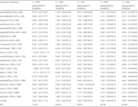
Table 4Coding performance of the proposed algorithm under different target complexities
Sequence (resolution) Tc= 90% Tc= 80% Tc= 70% Tc= 60% Tc= 50%
ΔBR/ΔPSNR/TS
(%/dB/%) Δ
BR/ΔPSNR/TS
(%/dB/%) Δ
BR/ΔPSNR/TS
(%/dB/%) Δ
BR/ΔPSNR/TS
(%/dB/%) Δ
BR/ΔPSNR/TS (%/dB/%)
BasketballPass (416 × 240) 0.76/−0.01/10.07 1.74/−0.02/20.00 3.57/−0.06/29.86 4.72/−0.07/39.79 6.24/−0.10/49.75
BlowingBubbles (416 × 240) 0.99/−0.01/13.77 1.45/−0.02/22.13 1.92/−0.06/31.31 2.21/−0.09/40.22 2.51/−0.13/49.41
BQSquare (416 × 240) 0.68/−0.00/10.08 1.46/−0.03/19.93 1.39/−0.08/30.30 2.82/−0.08/39.74 2.61/−0.15/49.37
RaceHorses (416 × 240) 0.77/−0.00/13.28 2.07/−0.04/22.46 3.28/−0.07/31.80 4.21/−0.10/40.95 5.44/−0.14/50.02
BasketballDrill (832 × 480) 0.51/−0.01/10.16 1.64/−0.02/20.05 2.82/−0.04/30.13 3.86/−0.06/39.75 5.04/−0.09/49.74
BasketballDrillText (832 × 480) 0.59/−0.01/10.26 1.62/−0.02/19.90 2.74/−0.06/30.24 3.69/−0.07/39.81 4.92/−0.10/49.66
BQMall (832 × 480) 0.54/−0.01/10.44 1.72/−0.02/22.34 3.32/−0.05/30.29 4.41/−0.08/40.14 5.73/−0.11/49.93
PartyScene (832 × 480) 0.76/−0.00/11.21 1.33/−0.02/20.16 1.84/−0.07/30.19 2.07/−0.12/39.72 2.58/−0.17/49.69
ChinaSpeed (1024 × 768) 0.44/−0.01/10.09 1.00/−0.02/20.10 1.32/−0.09/30.00 2.30/−0.11/39.74 3.20/−0.18/49.78
FourPeople (1280 × 720) 0.10/−0.00/10.15 0.24/−0.01/20.09 0.93/−0.02/30.14 0.83/−0.01/39.80 1.81/−0.03/49.84
Johnny (1280 × 720) −0.16/−0.01/11.72 0.13/−0.01/21.38 0.10/−0.02/31.21 0.51/−0.01/40.80 0.80/−0.03/50.03
KrustebAndSara (1280 × 720) 0.07/−0.01/9.98 0.46/−0.01/20.02 0.61/−0.03/30.06 1.07/−0.02/39.71 1.80/−0.05/49.50
SlideEditing (1280 × 720) 0.49/−0.01/13.62 0.44/−0.01/23.15 3.14/−0.04/32.25 2.87/−0.07/41.48 5.93/−0.12/50.47
SlideShow (1280 × 720) 0.09/−0.01/11.44 0.75/−0.04/20.91 3.00/−0.09/30.74 3.50/−0.13/40.81 6.98/−0.21/49.89
Vidyo1 (1280 × 720) −0.08/−0.01/10.99 0.04/−0.01/20.81 0.43/−0.02/30.45 0.32/−0.02/40.12 0.75/−0.04/49.62
Vidyo3 (1280 × 720) −0.11/−0.01/12.75 0.08/−0.01/22.13 0.73/−0.03/31.02 1.10/−0.02/40.67 1.81/−0.06/50.04
Vidyo4 (1280 × 720) 0.16/−0.00/13.00 0.13/−0.01/22.56 0.66/−0.02/31.27 0.83/−0.03/40.76 1.48/−0.04/49.98
BasketballDrive (1920 × 1080) 1.25/−0.01/10.55 2.32/−0.02/20.37 3.04/−0.03/30.24 3.76/−0.05/39.85 4.63/−0.06/49.62
BQTerrace (1920 × 1080) 0.64/−0.00/10.47 0.58/−0.02/20.52 −0.06/−0.03/30.34 1.19/−0.05/40.10 1.16/−0.07/49.90
Cactus (1920 × 1080) 0.33/−0.00/11.03 0.65/−0.01/20.27 1.68/−0.04/30.18 3.06/−0.06/40.10 3.35/−0.07/49.84
Kimono (1920 × 1080) 1.08/−0.01/10.92 0.95/−0.02/21.19 2.17/−0.02/30.84 3.27/−0.03/40.50 4.21/−0.04/50.21
ParkScene (1920 × 1080) 1.02/−0.00/10.80 1.98/−0.01/20.30 2.21/−0.04/30.33 4.59/−0.08/40.19 3.69/−0.07/49.97
Average 0.50/−0.01/11.22 1.04/−0.02/20.85 1.86/−0.05/30.60 2.60/−0.06/40.22 3.48/−0.09/49.83
The bit rate increase (ΔBR) and PSNR reduction (ΔPSNR) are used as measures of the rate distortion performance of the complexity control algorithm. The proposed algorithm tests and analyzes five target com-plexity levels,Tc(%) = {90, 80, 70, 60, 50}.
Table 4 summarizes the performance of the
pro-posed algorithm in terms of ΔPSNR, ΔBR, and TS for different sequences under different Tc. The experi-mental results presented in Table 4 indicate that the actual coding complexity of the proposed algorithm is quite close to the target complexity. This means that our algorithm can smoothly code most of the se-quences under limited computing power. Although the individual sequence deviation is large (when Tc = 90%, the maximal complexity deviation is 3.77%), the
MCE is small, with a maximum of 1.22%. For Tc =
90%, 80%, 70%, 60%, and 50%, the average ΔPSNR is
−0.01 dB, −0.02 dB, −0.05 dB, −0.06 dB, and −
0.09 dB, the average ΔBR is 0.50%, 1.04%, 1.86%,
2.60%, and 3.48%, and the MCE is 1.22%, 0.87%, 0.61%, 0.41%, and 0.24%, respectively. From the view-point of the degree of attenuation of the average ΔPSNR andΔBR with decreasingTc, the decrease of our algorithm is relatively smooth; however, the decrease of individual sequences is sharper (e.g., the sequence SlideShow, most of whose frames are smooth, except for some frames that have strong motion). This is because the frames with strong motion influence the CCA method, which depends on the encoding complexity of the previous frame.
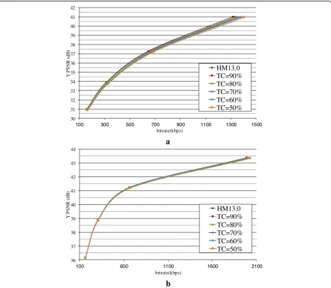
Figure 8 shows rate distortion curves of the
se-quence BasketballPass and Vidyo1 for the five
differ-ent Tc. The rate distortion performance of the
30 31 32 33 34 35 36 37 38 39 40 41 42
100 300 500 700 900 1100 1300 1500
Y P
S
N
R
(
d
B
)
bitrate (kbps)bitrate(kbps)
a
36 37 38 39 40 41 42 43 44
100 600 1100 1600 2100
Y P
S
N
R
(
d
B
)
bitrate (kbps) bitrate(kbps)
b
HM13.0 TC=90% TC=80% TC=70% TC=60% TC=50%
HM13.0 TC=90% TC=80% TC=70% TC=60% TC=50%
sequence BasketballPass with strong motion is not as good as the sequence Vidyo1, which has little scene changes. The conclusions also can be drawn from Table 4.
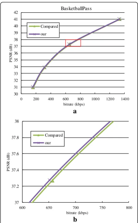
To demonstrate the effectiveness of our frame level complexity allocation method, two frame level
com-plexity allocation methods are compared in Tc =
90%. One of the methods is proposed in this paper, and the other is to get the target encoding time of the frame layer by equally dividing the target encod-ing time of the GOP layer. The same experimental environment described in first paragraph of this sec-tion was used for analyzing the performance of two methods, and the experimental results of the com-parison method are obtained by modifying the frame level complexity allocation method of the proposed
algorithm. As shown in Fig. 9, our method exhibits
better rate distortion performance, which proves that it can balance the complexity and rate distortion effectively in the frame layer.
To evaluate the performance of the proposed algo-rithm more intuitively, we compared our algoalgo-rithm with three state-of-the-art algorithms [14, 16, 17]. The results are listed in Tables 5, 6, and 7. Because the minimal controllable target complexity
propor-tions of [17] and our algorithm is 60% and 50%,
respectively, the performance is compared under the target complexity proportions, 80% and 60%.
Regarding losses in rate distortion performance, we
can find in Tables 5 and 7 that the average ΔBR of
our algorithm is slightly higher than [14, 17], and
the average ΔPSNR difference between our algorithm
and the algorithms [14, 17] is negligible when Tc =
80%. When Tc = 60%, the average rate distortion
performance of our algorithm is better than those of [14, 17]. Specially, for a few sequences, such as
Johnny, for which the performance our algorithm is slightly worse than that of [14, 17] in terms of both
ΔPSNR and ΔBR. It mainly benefits from the fact
that algorithms [14, 17] can effectively skip unneces-sary higher CU depths for little motion videos.
Moreover, we can find in Table 6 that the average
BDBR [19] of algorithm [16] is better than our algo-rithm, but the rate distortion performance of our al-gorithm is better in sequences of class E like Johnny
and FourPeople.
The control accuracy is an important index to
validate the performance of complexity control
algorithm, and the overall control accuracy of our algorithm and other three algorithms is compared by MCE. From Tables 5, 6, and 7, we can obviously see that the MCE of our algorithm is lower than [14, 16,
17], which means that our algorithm can achieve
steady complexity control for different test sequences.
5 Conclusions
This paper proposed a hierarchical complexity control algorithm based on the coding unit depth decision to guarantee the rate distortion performance during real-time coding when the computing power of a device is limited. First, we get the reference time by periodical updating strategy. Second, the GOP layer and frame layer complexity allocation and control method based on the target complexity are used to control the coding time of these layers. Then, the RDO process at unnecessary CU depths layer is skipped by using the correlation between ESAD and the optimal depth and by establishing the ECDM model to adaptive allocate the maximum CTU depth. Next, based on the CU smoothness decision and the
30 31 32 33 34 35 36 37 38 39 40 41 42
0 200 400 600 800 100 0 120 0 140 0
PS
N
R
(
d
B
)
bitrate (kbps)
BasketballPass
Compared
our
37 37.2 37.4 37.6 37.8 38
600 650 700 750 800
PSN
R
(
d
B
)
bitrate (kbps)
Compared
our
a
b
Fig. 9Comparison of rate distortion performance between the proposed frame level complexity allocation method and the average complexity allocation method forsequence BasketballPasswith 90% target complexity proportion.aRate distortion performance.b
Table 5Performance comparison between the proposed algorithm and [14]
Sequence (class) Our HM13.0 [14] HM16.0
Tc= 80% Tc= 60% Tc= 80% Tc= 60%
ΔBR/ΔPSNR/TS (%/dB/%) ΔBR/ΔPSNR/TS (%/dB/%) ΔBR/ΔPSNR/TS (%/dB/%) ΔBR/ΔPSNR/TS (%/dB/%)
BasketballDrive (B) 2.32/−0.02/20.37 3.76/−0.05/39.85 0.33/−0.03/21.42 2.02/−0.15/39.76
BQTerrace (B) 0.58/−0.02/20.52 1.19/−0.05/40.10 0.33/−0.02/20.25 3.20/−0.08/38.10
ParkScene (B) 1.98/−0.01/20.30 4.59/−0.08/40.19 0.60/−0.03/20.00 5.87/−0.14/38.73
Johnny (E) 0.13/−0.01/21.38 0.51/−0.01/40.80 −0.05/0.00/19.16 0.02/0.00/40.90
FourPeople (E) 0.24/−0.01/20.09 0.83/−0.01/39.80 0.13/0.00/19.07 0.44/−0.01/39.77
Vidyo1 (E) 0.04/−0.01/20.81 0.32/−0.02/40.12 0.03/0.00/18.02 0.62/−0.02/37.81
Vidyo3 (E) 0.08/−0.01/22.13 1.10/−0.02/40.67 0.04/0.00/18.89 1.55/−0.05/36.64
Vidyo4 (E) 0.13/−0.01/22.56 0.83/−0.03/40.76 0.15/0.00/17.72 0.21/−0.01/38.99
PartyScene (C) 1.33/−0.02/20.16 2.07/−0.12/39.72 2.53/−0.10/21.27 8.29/−0.25/39.50
RaceHorsesC (C) 1.48/−0.03/22.45 2.86/−0.07/40.93 1.56/−0.08/21.69 7.37/−0.45/41.87
BasketballDrill (C) 1.64/−0.02/20.05 3.86/−0.06/39.75 0.46/−0.02/17.25 4.85/−0.18/37.29
SlideEditing (F) 0.44/−0.01/23.15 2.87/−0.07/41.48 0.42/−0.03/18.47 3.32/−0.30/38.94
SlideShow (F) 0.75/−0.04/20.91 3.50/−0.13/40.81 0.40/−0.03/19.82 0.58/−0.06/38.00
Average 0.86/−0.02/21.14 2.18/−0.06/40.38 0.53/−0.02/19.46 2.95/−0.13/38.95
MCE 1.14% 0.52% 1.25% 1.48%
Table 6Performance comparison between the proposed algorithm and [16]
Sequence (class) Our HM13.0 [16] HM16.9
Tc= 80% Tc= 60% Tc= 80% Tc= 60%
BDBR/TS (%/%) BDBR/TS (%/%) BDBR/TS (%/%) BDBR/TS (%/%)
Kimono (B) 1.84/21.19 4.18/40.50 0.44/23.39 0.98/41.65
ParkScene (B) 2.05/20.30 5.79/40.19 0.32/24.60 1.76/42.79
Cactus (B) 1.07/20.27 5.59/40.10 0.17/24.54 1.72/42.59
BasketballDrive (B) 3.34/20.37 5.95/39.85 0.23/21.20 1.95/38.99
BQTerrace (B) 1.67/20.52 3.96/40.10 0.28/21.67 2.02/40.43
BasketballDrill (B) 2.24/20.05 5.38/39.85 0.29/20.56 2.60/39.54
BQMall (C) 2.27/22.34 6.60/40.14 0.59/24.59 2.98/42.90
PartyScene (C) 1.83/20.16 5.31/39.72 0.17/21.28 1.43/39.92
RaceHorsesC (C) 2.08/22.45 4.64/40.93 0.30/23.39 1.95/41.57
BasketballPass (D) 2.32/20.00 6.30/39.79 0.64/26.90 2.08/44.21
BQSquare (D) 2.08/19.93 4.89/39.74 0.02/19.08 1.44/38.65
BlowingBubbles (D) 1.96/22.13 4.56/40.22 0.42/22.71 1.90/40.73
RaceHorses (E) 2.93/22.46 6.72/40.95 0.52/23.40 1.35/41.73
FourPeople (E) 0.50/20.09 1.06/39.80 1.24/19.90 3.06/39.11
Johnny (E) 0.32/21.38 0.86/40.80 1.32/19.29 2.64/38.04
KristenAndSara (E) 0.45/20.02 1.55/39.71 1.10/19.47 2.58/39.07
Average 1.81/20.85 4.58/40.15 0.50/22.27 2.03/40.75
adaptive low bit threshold decision, the redundant traversal process within the allocated maximal depth is reduced to further save the time. Finally, the adap-tive upper bit threshold is used to guarantee the qual-ity of important CUs by performing the RDO process at depths larger than the maximal depth allocated by the CCA method. The experimental results showed that the minimum target complexity of our algorithm
can reach 50% with smooth attenuation of ΔPSNR
and ΔBR as Tc decreases. Compared with other
state-of-the-art complexity control algorithms, our al-gorithm outperforms better in control accuracy. In the future, we will design an effective mode decision method to save more time. In addition, we will fur-ther investigate the frame layer complexity allocation and improve the frame layer control accuracy.
Abbreviations
ABD:Adaptive upper and lower bit threshold decision; CCA: CTU complexity allocation; CSD: CU smoothness decision; CTU: Coding tree unit; CU: Coding unit; ECDM: Complexity-depth model; ESAD: Effective sum of absolute
differences; FDM: Fast decision for merge rate-distortion cost; FEN: Fast encoder decision; GOP: Group of picture; HEVC: High Efficiency Video Coding; HM: HEVC test model; JCT-VC: Joint Collaborative Team on Video Coding; MAD: Mean absolute difference; MPEG: Moving Picture Experts Group; PB: Prediction block; PU: Prediction unit; QP: Quantization parameters; RDO: Rate distortion optimization; SAO: Sample adaptive offsets;
TB: Prediction block; TU: Transform unit; VCEG: Video Coding Experts Group
Acknowledgements
The authors would like to thank the editors and anonymous reviewers for their valuable comments.
Funding
This work is supported by the Natural Science Foundation of China (61771269, 61620106012, 61671258) and Natural Science Foundation of Zhejiang Province (LY16F010002, LY17F01000 5). It is also sponsored by K.C. Wong Magna Fund in Ningbo University.
Availability of data and materials
The conclusion and comparison data of this article are included within the article.
Authors’contributions
FC designed the proposed algorithm and drafted the manuscript. PW carried out the main experiments. ZP supervised the work. GJ participated in the algorithm design. MY performed the statistical analysis. HC offered useful Table 7Performance comparison between the proposed algorithm and [17]
Sequence (class) Our HM13.0 [17] HM13.0
Tc= 80% Tc= 60% Tc= 80% Tc= 60%
ΔBR/ΔPSNR/TS (%/dB/%) ΔBR/ΔPSNR/TS (%/dB/%) ΔBR/ΔPSNR/TS (%/dB/%) ΔBR/ΔPSNR/TS (%/dB/%)
BasketballPass (D) 1.74/−0.02/20.00 4.72/−0.07/39.79 1.11/−0.06/20.44 4.84/−0.25/35.15
BlowingBubbles (D) 1.45/−0.02/22.13 2.21/−0.09/40.22 2.26/−0.08/20.43 11.79/−0.47/43.75
BQSquare (D) 1.46/−0.03/19.93 2.82/−0.08/39.74 1.40/−0.05/17.75 12.74/−0.58/39.14
RaceHorses (D) 2.07/−0.04/22.46 4.21/−0.10/40.95 0.92/−0.05/13.77 15.42/−0.78/38.92
BasketballDrill (C) 1.64/−0.02/20.05 3.86/−0.06/39.75 0.79/−0.02/17.06 5.19/−0.24/39.76
BasketballDrillText (C)
1.62/−0.02/19.90 3.69/−0.07/39.81 0.75/−0.03/17.28 6.35/−0.30/41.12
BQMall (C) 1.72/−0.02/22.34 4.41/−0.08/40.14 0.71/−0.03/20.78 12.20/−0.49/46.59
PartyScene (C) 1.33/−0.02/20.16 2.07/−0.12/39.72 3.62/−0.17/21.18 25.05/−1.02/52.67
ChinaSpeed (E) 1.00/−0.02/20.10 2.30/−0.11/39.74 0.89/−0.07/21.15 26.67/−1.38/42.66
FourPeople (E) 0.24/−0.01/20.09 0.83/−0.01/39.80 0.16/−0.01/20.93 0.66/−0.02/44.46
Johnny (E) 0.13/−0.01/21.38 0.51/−0.01/40.80 0.08/−0.00/19.35 −0.10/−0.00/39.44
KrustebAndSara (E) 0.46/−0.01/20.02 1.07/−0.02/39.71 −0.18/−0.00/18.39 0.12/−0.00/39.08
SlideEditing (F) 0.44/−0.01/23.15 2.87/−0.07/41.48 0.23/−0.02/17.66 0.48/−0.07/42.49
SlideShow (F) 0.75/−0.04/20.91 3.50/−0.13/40.81 0.50/−0.04/16.58 6.97/−0.54/35.56
Vidyo1 (E) 0.04/−0.01/20.81 0.32/−0.02/40.12 0.24/−0.01/18.61 0.26/−0.01/39.48
Vidyo3 (E) 0.08/−0.01/22.13 1.10/−0.02/40.67 −0.17/−0.00/15.93 0.46/−0.01/41.46
Vidyo4 (E) 0.13/−0.01/22.56 0.83/−0.03/40.76 0.01/−0.00/18.07 0.87/−0.04/44.83
BasketballDrive (B) 2.32/−0.02/20.37 3.76/−0.05/39.85 0.32/−0.01/17.10 1.72/−0.05/38.21
BQTerrace (B) 0.58/−0.02/20.52 1.19/−0.05/40.10 0.59/−0.02/20.60 7.92/−0.25/54.10
Cactus (B) 0.65/−0.01/20.27 3.06/−0.06/40.10 0.14/−0.01/14.91 2.42/−0.08/39.58
Kimono (B) 0.95/−0.02/21.19 3.27/−0.03/40.50 0.29/−0.01/19.69 1.07/−0.04/42.06
ParkScene (B) 1.98/−0.01/20.30 4.59/−0.08/40.19 0.57/−0.03/19.51 7.28/−0.31/48.62
Average 1.04/−0.02/20.85 2.60/−0.06/40.22 0.69/−0.03/18.50 6.83/−0.31/42.23
suggestions and helped to modify the manuscript. All authors read and approved the final manuscript.
Competing interests
The authors declare that they have no competing interests.
Publisher’s Note
Springer Nature remains neutral with regard to jurisdictional claims in published maps and institutional affiliations.
Received: 22 March 2018 Accepted: 18 September 2018
References
1. G.J. Sullivan, J.-R. Ohm, W.-J. Han, T. Wiegand, Overview of the high efficiency video coding (HEVC) standard. IEEE Trans. Circuits Syst. Video Technol.22(12), 1649–1668 (2012)
2. T. Wiegand, G.J. Sullivan, G. Bjøntegaard, A. Luthra, Overview of the H.264/ AVC video coding standard. IEEE Trans. Circuits Syst. Video Technol.13(7), 560–576 (2003)
3. I.-K. Kim, K. Mccann, K. Sugimoto, B. Bross, W.-J. Han, G. Sullivan,High Efficiency Video Coding (HEVC) Test Model 13 (HM13) Encoder Description ITU-T/ISO/IEC Joint Collaborative Team on Video Coding (JCT-VC) Document JCTVC-O1002, in 15th Meeting of JCT-VC(CH, Geneva, 2013)
4. T.K. Tan, R. Weerakkody, M. Mrak, N. Ramzan, V. Baroncini, J.-R. Ohm, G.J. Sullivan, Video quality evaluation methodology and verification testing of HEVC compression performance. IEEE Trans. Circuits Syst. Video Technol.
26(1), 76–90 (2016)
5. J.-R. Ohm, G.J. Sullivan, H. Schwarz, T.K. Tan, T. Wiegand, Comparison of the coding efficiency of video coding standards—including high efficiency video coding (HEVC). IEEE Trans. Circuits Syst. Video Technol.22(12), 1669– 1684 (2012)
6. R. Fan, Y. Zhang, B. Li, Motion classification-based fast motion estimation for high-efficiency video coding. IEEE Trans. Multimedia.19(5), 893–907 (2017) 7. J. Zhang, B. Li, H. Li, An efficient fast mode decision method for inter prediction
in HEVC. IEEE Trans. Circuits Syst. Video Technol.26(8), 1502–1515 (2016) 8. F. Chen, P. Li, Z. Peng, G. Jiang, M. Yu, F. Shao, A fast inter coding algorithm
for HEVC based on texture and motion quad-tree models. Signal Process. Image Commun.44(C), 271–279 (2016)
9. G. Correa, P. Assuncao, L. Agostini, L.A. da Silva Cruz, Computational complexity control for HEVC based on coding tree spatio-temporal correlation (IEEE 20th International Conference on Electronics, Circuits, and Systems (ICECS), Abu Dhabi, United Arab Emirates) (2013), pp. 937–940 10. G. Correa, P. Assuncao, L. Agostini, L.A. da Silva Cruz, Coding tree depth
estimation for complexity reduction of HEVC (2013 data compression conference, Snowbird, UT, USA) (2013), pp. 43–52
11. G. Correa, P. Assuncao, L. Agostini, L.A. da Silva Cruz, Complexity scalability for real-time HEVC encoders. J. Real.-Time Image Process.12(1), 107–122 (2016) 12. G. Correa, P. Assuncao, L. Agostini, L.A. da Silva Cruz, Encoding time control
system for HEVC based on rate-distortion-complexity analysis (2015 IEEE International Symposium on Circuits and Systems (ISCAS), Lisbon, Portugal) (2015), pp. 1114–1117
13. X. Deng, M. Xu, L. Jiang, X. Sun, Z. Wang, Subjective-driven complexity control approach for HEVC. IEEE Trans. Circuits Syst. Video Technol.26(1), 91–106 (2016)
14. X. Deng, M. Xu, C. Li, Hierarchical complexity control of HEVC for live video encoding. IEEE Access.4(99), 7014–7027 (2016)
15. X. Deng, M. Xu, Complexity control of HEVC for video conferencing (2017 IEEE International Conference on Acoustics, Speech and Signal Processing (ICASSP), New Orleans, LA, USA) (2017), pp. 1552–1556
16. J. Zhang, S. Kwong, T. Zhao, Z. Pan, CTU-level complexity control for high efficiency video coding. IEEE Trans. Multimedia.20(1), 29–44 (2018) 17. A. Jiménez-Moreno, E. Martínez-Enríquez, F. Díaz-De-María, Complexity
control based on a fast coding unit decision method in the HEVC video coding standard. IEEE Trans. Multimedia.18(4), 563–575 (2016) 18. F. Bossen,Common Test Conditions and Software Reference Configurations,
ITU-T/ISO/IEC Joint Collaborative Team on Video Coding (JCT-VC) Document JCTVC-H1100, in 8th Meeting of JCT-VC(CA, San Jose, 2012)