2D face recognition techniques by

112404-5858 IJVIPNS-IJENS © August 2011 IJENS _{I J E N S} 

Abstract— This paper presents a passive stereo vision face recognition system which uses stereo camera to detect and recognize a person’s face. The propose algorithm improves classical monocular 2D face recognition techniques by additionally considering the facial 3D surface, which is rather stable under various illumination conditions. Initially, individual faces are detected and their facial 3D surfaces are reconstructed from the stereo images. Next, the 3D face is then composed into its 2D image data with appropriate depth data and then decomposed into its principle components. The principle components are used to recognize a 3D face by comparing characteristics of the current face to those faces available in database. The results of our approach show a good improvement in recognition rate. For evaluation purposes, we then compared the performance of our approach to a classical face recognition algorithm and observed that the recognition rate increased on average by 9.03 percent.

Index Term— Stereo vision, fuzzy clustering, principle component analysis, face recognition

I. INTRODUCTION

FACE recognition has been widely applied in computer vision and pattern recognition areas. Face recognition was first developed by Bledsoe [1], uses only geometry relationship to detected facial features in monocular 2D images to identify a person. Then during the 90’s, Turk and Pentland [2] proposed a new approach using eigenface value for face recognition. The method in [2] which is based on Principle Component Analysis (PCA) was later refined by Frey et al. [3].

PCA is defined by its capabilities to transform a number of possible correlated variables into a small number of uncorrelated variables known as principle component. By expressing the data this way, their similarity ratio can be observed. Monocular 2D face recognition method suffer from limited input data and insufficient information due to it nature on evaluating only 2D images region which are not invariant under various illumination condition.

Tsalakanidou et al. [4] introduced the application of depth information to improved face recognition. Wang et al. [5] proposed an approach using morphological filter with combination of some heuristics method to detect the closest face to the camera. Therefore, only single face is detectable

Lim Eng Aik is with Institut Matematik Kejuruteraan, Universiti Malaysia Perlis, 02000 Kuala Perlis, Perlis, Malaysia (Phone: 985-5485; fax:

604-985-5432; e-mail: ealim@ unimap.edu.my).

Tan Wee Choon is with School of Mechatronic Engineering, Universiti Malaysia Perlis, Ulu Pauh, 02600 Arau, Perlis, Malaysia (E-mail:

[email protected]).

and analyzed. Recently, a number of face recognition methods using 3D information were reported [6, 7], but none of these 3D face recognition method approaches is capable to detect and recognize multiple person or non-person from photo print person found in images.

Our proposed approach uses Fuzzy C-means clustering (FCM) and 3D depth information to significantly improve the recognition rate. Furthermore, it capable of detect and recognize multiple person or none-person in images. The depth information from the stereo images is estimated using a fast variational disparity solver. Subsequently, FCM is applied on the disparity vector to reduce the input sizes and fasten the detection and recognition process. Then, the 2D image intensity and depth information at each face point are transformed into Principle Component Analysis (PCA) space.

Therefore, two separate PCA transformation is calculated, one for the image intensity and one for the depth information. The incoming 3D face is transformed to PCA space and the Mahalanobis distance (MD) to each trained faces is calculated. If the MD is small enough, the system classifier will return the person whose face has the smallest MD to the current one; otherwise, if the MD is too large, the system will classifies that person as new face, and will be added to PCA database. In our experiments, there are 50 persons store within the PCA database.

II. OVERVIEW OF SYSTEM

Fig. 1 gives an overview of our propose face recognition system. The input consists of a sequence of stereo image pairs and the output is a listed of person that are recognized in current image. The system consists of four major blocks: disparity estimation, clustering section, PCA face detection, and face recognition. Our approach for disparity estimation and face detection is summarized in the next section. Section 4 introduces the PCA and FCM approach for face recognition. In Section 5, we evaluate our proposed approach and the paper ends with a conclusion.

Enhancing Passive Stereo Face Recognition

using PCA and Fuzzy C-Means Clustering

Fig. 1. Overview of our propose face recognition system.

III. DISPARITY ESTIMATION AND FACE DETECTION The stereo image pair acquire by using two cameras with an image resolution of 320 x 240 pixels. Both cameras are mounted next to each other with baseline distance of 10 cm and an angle of convergence of 10 degrees. After complete calibration task on the cameras, we rectify the input images to standard stereo geometry and estimate it disparity map.

To perform the disparity estimation, we choose the Sum of Absolute Difference (SAD) by [8] to compute its correlation values. To implement the algorithm effectively, a three dimensional Disparity Space Image (DSI) [9] is constructed. The cuboids dimension is determined by the width and height of the images, and the disparity search range. Each position (x, y, d) in the cuboids memory denoted the absolute difference value between the value at position (x, y) in the left image and the value at the position (x + d, y) in the right image (Fig. 2).

After DSI is computed, an initial dense disparity map is calculated. An array DSI (x, y, d) has an absolute difference value at position of (x, y) and disparity d. (1) expresses the mathematical form of SAD.

 

 

   

1 1

1 1

2 2

1 1

1 1

2 2

SAD( , , )

( , ) ( , )

x y

x y

w w

L R

i w j w x y d

I x i y j I x i d y j

 

   



 

      (1)

where IL and IR are the left and right images respectively, and wx and wy are the sub-correlation window size for left and right images respectively. The disparity at (x, y), d(x, y), is the point where minimum correlation value of SAD is found. Consequently, the disparity value is calculated as follows:

min max

( , ) arg min SAD( , , ) d d d

d x y x y d

 

 (2)

Then, we apply the left/right consistency check [10]. The left and right disparities should satisfy (3). DR(x, y) and DL(x, y) are the disparity at (x, y) in right and left images respectively. If (3) is not satisfied, then DL(x, y) turn out to be invalid and a value -1 is assigned as replacement.

( ( , ), ) ( , )

R L L

D xD x y y  D x y (3)

The faces are detected using a stereo-enhanced face detection algorithm in [11]. For each detected face, we extract the face region and it corresponding disparity map (Fig. 3). Each region is scaled to resolution of N x N pixels with N = 60 in our experiments. For each face region, we extract two matrices with N x N elements. The first matrix contains image intensities, and the second matrix consists of disparity values. Each matrix is separated. The rows of the matrix are resembles into N2 x 1 vector. As a result, we obtain two N2 x 1 vectors, the intensity vector x and the disparity d for each detected face. FCM clustering is then performed on these two vectors to reduce the vector size by 50 percent.

Fig. 2. Three-dimensional disparity space image [9].

Fig. 3. Example of extracted face and their corresponding disparity map.

IV. FACE RECOGNITION

For face recognition task, we applied PCA [12] which capable of creating the face subspace, defined as orthogonal basis of vectors that contains the most relevant information about a face. These vectors are the eigenvectors of the covariance matrix of the distribution that covered by the training set of faces. Hence, new face can be projected into the face subspace which represented by a linear combination of these eigenvectors. The recognition process is achieved by representing new face as a point in face subspace, and then computes the distances between these points to other points which correspond to the known faces in the training set.

In this work, we used a training set of K = 417 faces with corresponding disparity maps (Fig. 3). We test our propose approach with testing set data of 120 faces. Each image has a resolution of N x N pixels.

A. Principle Component Analysis (PCA)

Let x_k as the intensity vectors and d_k as the disparity

112404-5858 IJVIPNS-IJENS © August 2011 IJENS _{I J E N S} 1 1 K k k x x K 





is computed. The average face x and the

corresponding disparity map d are shown in Fig. 3. Subsequently, the N2 x N2 covariance matrix C describing the variation in our dataset is given by

1 1 ( )( ) K T k k k

C x x x x

K 





  (4)

The covariance matrix C is a symmetrical matrix with a

spectral decomposition of the form C U UT, where U is an orthogonal matrix and is a diagonal matrix [13]. The columns of U are the eigenvectors of C and the diagonal elements , are the eigenvalues. The eigenvectors in U are sorted in ascending order to their corresponding eigenvalues. The eigenvectors are also known as principle components.

The eigenvector with the highest eigenvalue is the principle component of data set which describes the most significant relationship between data dimensions. The average face and the face constructed for our data set are shown in Fig. 4. Eigenvectors with small singular values contain less information on the variance of our dataset which can be dropped without losing information. Thus, the resulting face space will have fewer dimensions than the original one.

The PCA transformed a N2 x 1 input vector x to a N x 1 (N= K in this experiment) vector y in face space can now be

performed with yUT(xx). Therefore, our K training

vector

x

_k into PCA space with

( ), 1,...,

T

k k

y U x x  k K (5)

To compute the weighted distance of the face, given by an input vector x, we have to calculate y and compare it with all transform vectors y_k. We then calculate the Mahalanobis

distance using (yy_k)T_y1(yy_k). Therefore, the NxN

matrix _yis the reduce version of matrix that contains only

the N largest eigenvalues.

In order to obtain an even better result during PNN classification, we employ the disparity information. Based on

(5), the disparity vector d_kof the training set are projected into

PCA space given by V:

( ), 1,..., .

T

k k

e V d d  k K (6)

To obtain the input vector for a face, we now calculate the weighted Mahalanobis distance, W, as follow:

1 1

( )T ( ) (1 )( )T ( )

k y k k e k

W  yy  yy   ee  ee (7)

for all k = 1,…,K and return as the face distance vector.

Fig. 4. Disparity map estimation and 3D face reconstruction: a) left frame of stereo image, b) reconstructed disparity map, c) corresponding depth-map on 3D grid, d) average face constructed from depth-map, e) reconstructed 3D

face.

B. Fuzzy C-Means Clustering (FCM)

The Fuzzy C-means (FCM) algorithm was originally developed by Dunn [14], and later generalised by Bezdek [15]. To describe the algorithm, we set some notations. The set of all points considered is X = {x1, x2, …, xn}. We write

: [0,1]

i

u X  for the i-th cluster, i =1,…,c, and we will use

uik to denote ui(xk), i.e. the grade of membership of xk in cluster

ui. We use U  uik for the matrix of all membership values.

The midpoint of ui is vi, and is computed according to

1 1 n m ik k k i n m ik k U x v U   





(8)

A parameter m, 1m , will be used as a weighted exponent, and the particular choice of value m is application dependent [16]. For m = 1, it coincides with the FCM algorithm, and if m , then all uik values tend to 1/c [17]. Membership in fuzzy clusters must fulfil the condition

1

1,

1,...,

c

ik i

U

k

n



  



(9)

i.e. for each x



X, the sum of memberships of x in respective ci

must be 1. A typical distance measure  is the Euclidean distance.

The objective of the clustering algorithm is to select ui so as to minimize the objective function

 

2

1 1

m c n

ik k i i k

J u x v

 





 (10)

The following algorithm for FCM clustering will meet this objective:

1. Fix c and m. Initialise U to some U(1). Select



0for stopping condition.

2. Update midpoint values vi for each cluster ci.

3. Compute the set_k 



i: 1 i c: x_k v_i 0



, and update U( )according to the following: if_k ,

then





  2 1 1 1 m c

ik k i k j

j

x v x v











_

 



_







, otherwise

0,

ik i k

    and

1

k

ik i









. (



i: 1 i c: x_k v_i 0



).

4. Stop if J



, otherwise go to step 2.

In step 1, c( 1 ) is set to a fixed number of clusters. In the rule generation phase, each cluster will be the basis for one rule. Usually we keep c as small as possible in order to keep the number of rules within reasonable bounds. Further, the

matrix U  u_ik is to be initialized. A crisp, and even

random, partition of X into c subsets can be sufficient to provide a good starting point for the algorithm.

In step 2, midpoint values vi are computed, and respective midpoints will of course move towards points with higher membership values in their clusters. Note that a midpoint can

coincide with some

x

_. In such a case we will have u_i 1,

and then, for all  i, we will have u_ 0.

Step 3 is the core of the algorithm. There, membership values uik are updated. Note that we must distinguish between cases depending on whether or not midpoints coincide with data points. The variable denotes the iteration number.

In step 4, we compute the difference between present and previous matrices of membership values. If the stopping condition is met, we are done.

V. EXPERIMENT AND RESULTS

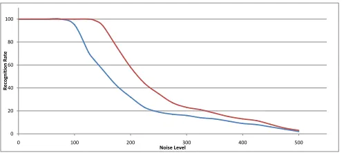
The proposed model approach was tested on 200 images input samples consists of different faces or non-faces are used during the training with PCA database of 417 faces in order to evaluate our approach. We repeated this experiment two times: 1) for classical monocular PCA based face recognition algorithm, 2) for our FCM-PCA face recognition that used reduced version of disparity information as training input. Furthermore, we repeated the experiment for different noise

levels of variance 2 perturbed by Gaussian noise. Fig. 5 compares the recognition rates for the two approaches.

Additional feature of our proposed approach is that it can not be deceive by a photo print of a person. Table I shows the timings for the different steps of our algorithm are given. On average, overall noise levels, the propose approach improves the recognition rate by 9.03 percent compare to classical monocular approach.

0 20 40 60 80 100

0 100 200 300 400 500

R

e

co

gn

ition

R

ate

Noise Level

Fig. 5. Recognition rate (in percent) over noise level



for the classic monocular recognition (green), and our propose FCM-PCA method (red).

TABLEI

Timings for the algorithms using Intel Core 2 Duo CPU with 2.66 GHz

Step Mono (msec) Stereo (msec)

Estimate disparity map - 104

FCM - 7

Face detection 126 164

Face recognition 2 2

Total 128 277

VI. CONCLUSION

In this paper, a PCA based algorithm is extended by additionally applying FCM for reducing the input sizes to fasten the detection and recognition processes. The system correctly recognized faces by 9.03 percent on average. This work shows that it is beneficial to use disparity information provided by stereo camera system for improving recognition rate. Additional feature of our approach in practice is that it can differentiate between real faces and photos of faces due to photo has a flat surface. This makes it more difficult to fake an identity and this is especially important, if the application of face recognition software is data encryption or security.

REFERENCES

[1] W.W. Bledsoe, “The model method in facial recognition,” Tech. Report 15, Panoramic Research Inc., Palo Alto, CA, 1997.

[2] M.A. Turk, A.P. Pentland, “Face recognition using eigenfaces,” In:

Proc. IEEE Computer Vision and Pattern Recognition, pp. 586-591, 1991.

[3] B.J. Frey, A. Colmenarez, T.S. Huang, “Mixtures of local linear subspaces for face recognition,” In: Proc. IEEE Conference on Computer Vision and Pattern Recognition, pp. 32-37, 1998.

[4] F. Tsalakanidou, D. Tzovaras, M.G. Strintzis, “Use of depth and color eigenfaces for face recognition,” Pattern Recognition Letter, 24, no. 9-10, pp. 1427-1435, 2003.

[5] J.G. Wang, E.T. Lim, X. Chen, R. Venkateswarlu, “Real-time stereo face recognition by fusing appearance and depth fisherfaces,” Journal of VLSI Signal Process System, 49, no. 3, pp. 409-423, 2007.

[6] A. Hayasaka, K. Ito, T. Aoki, H. Nakajima, K. Kobayashi, “A robust 3d face recognition algorithm using passive stereo vision,” In: Proc.IEICE Transactions92-A, no. 4, pp. 1047-1055, 2009.

[7] T.H. Sun, M. Chen, S. Lo, F.C. Tien, “Face recognition using 2D and disparity eigenfaces,” Expert System and Applications, 33, no. 2, pp. 265-273, 2007.

[8] O. Faugeras, B. Hotz, H. Mathieu, T. Vieville, Z. Zhang, P. Fua, E. Theron, L. Moll, G. Berry, J. Vuillemin, P. Bertin, C. Proy, “Real-time correlation-based stereo: algorithm, implementations, and application,”

INRIA, Technical Report, no. 2013, 1993.

[9] K. Muhlmann, D. Maier, J. Hasser, R. Manner, “Calculating dense disparity maps from colour stereo images, an efficient implementation,”

Internet Journal of Computer Vision, 47, pp. 79-88, 2002.

[10] P. Fua, “A parallel stereo algorithm that produces dense depth maps and preserves image features,” Machine Vision Application, 6, pp. 35-49, 1993.

[11] K. Sergey, S. Kristina, K. Faber, T. Thorsten, H.P. Seidel, “Rapid stereo-vision enhanced face detection,” In: Proc. IEEE International Conference on Image Processing,pp. 1221-1224, 2009.

112404-5858 IJVIPNS-IJENS © August 2011 IJENS _{I J E N S} [13] W.H. Press, S.A. Teukolsky, W.T. Vetterling, B.P. Flannery,

“Numerical Recipes in C++: The art of scientific computing,” Cambridge University Press, 2002.

[14] J.C. Dunn, “A fuzzy relative of ISODATA process and its use in detecting compact well separated clusters,” Journal of Cybernetics, 3, pp. 32-57, 1973.

[15] J.C. Bezdek, “Cluster validity with fuzzy sets,” Journal of Cybernetics, 4, pp. 58-73, 1974.

[16] J.C. Bezdek, “Pattern recognition with fuzzy objective function algorithms,” Plenum, New York, 1981.