Constrained GA Based Online PI Controller
Parameter Tuning for Stabilization of Water Level in
Spherical Tank System
S.P.Selvaraj
1, A.Nirmalkumar
21Deparmemt of Electronics and Instrumentation Engineering, Bannari Amman Institute of Technology, sathyamanagalam, Tamilnadu, India-638401.Ph: +91-4295 226227, Fax:+91-4295226666 [email protected]
2 Principal, Karpagam College of Engineering, Myleripalayam Village, Coimbatore, Tamilnadu, India- 641032. Ph: +91-422 2619047, Fax: +91- 422 2619046, [email protected]
Abstract— Level Control of spherical tank is one of the requirements in industries, where the storage of large volumes of highly pressurized liquids takes place. The level control in spherical tank is cumbersome due to variation of cross sectional area with respect to its height. In the proposed work, PI controller is used to control the level of spherical tank. Initially, the Ziegler Nicholas step response method is used to geta first order plus dead time mathematical model and single set of PI parameter.Multiple models or multiple sets of PI controller parameters are also obtained at different operating points using Z-N and online CGA based tuning methods. By conducting experimental study, the servo and regulatory responses of the spherical tank process are obtained with the controller parameters obtained through various tuning methods.The online CGA based tuning method produce better output response with minimum Integral Square Error (ISE) and Integral Absolute Error (IAE) in real-time, with respect to set point and load changes.
Index Term— Constrained GA, PI controller, Spherical Tank, Online tuning, IAE and ISE.
I. INTRODUCTION
Liquid level control is one of the important schemes in many products and process industries including manufacturing, storage and service industries to get product accuracy, safety and reduce energy consumption. Proportional-Integral-Derivative (PID) controller is the most used continuous controllers in the industry and universally accepted control algorithm for industrial control due to its robust performance, functional simplicity and operator friendly. The PID controllers can be implemented tocontrol a variable at any given operating point within an acceptable degree of accuracy, which eliminates the need for continuous operator attention. Basically the level process has fast output response, single energy storage element (capacitive), considerable disturbance and transportation lag. The use of proportional control may require a large gain to minimize the steady state error and the increase in gain will reduce the system stability. The PI action offers both fast response and zero steady state error due to the proportional and integral actions respectively. So, the Proportional-Integral (PI) controller is commonly used to control the level processes in industries.
The PI controller or PID controller performance is based on its parameters controller gain (Kc), Integral/reset time (Ti) and derivative time (Td). In industries, trial and error method is used to assign the controller parameters and analyze the response of the process. After analysis the parameters are adjusted manually to improve the responses and this kind of parameter selection is cumbersome even though the process tank is linear. A tuning method is essential in order to select suitable PI controller parametersfor the proposed level control scheme, because small step change also introduce considerable oscillations in the process due to variation in the cross section of the tank.
Anandanatarajan R et al (2006) has tuned the controller parameter at a nominal operating point using Ziegler-Nichols Proportional Integral (ZNPI) controller method and response of nonlinear systems has been obtained. A simulation study has been conducted for the system using Non-Linear PI (NLPI) controller and it produced less oscillatory response [1]. The NLPI controller is implemented only in simulation, in real time the NLPI controller may behave differently due to process dynamics. Nithya S et al (2008) has implementedan Internal Model Control (IMC) and Skogestad’s IMC (SIMC) for level control of spherical tank, at four different operating points and it was concluded that the IMC and SIMC based tuning exhibits minimum overshoot with faster settling time when compared to ZN tuned controller for set point and load changes [8]. The result shows that IMC controller also exhibits considerable overshoot. This method requires a mathematical model for each operating point and it is difficult to get mathematical model for each operating point of a spherical tank in real time.
technique and implementing them in real time may not give robust performance.So, intelligent tuning algorithms are essential to tune the parameters [2].
Genetic algorithms (GAs) are search algorithms based on the mechanics of natural selection and natural genetics. GAs has been applied to a wide range of optimization problemsto find optimum solutions and the PI controller requires best possible parameters to produce satisfactory response. Hence, they are admirably suited to the controller parameter tuning. Constraints are added in the GA during population initialization and mutation process in order to reduce the tuning period and keep the process variable in a specified limit. After adding constraints, the algorithm is named as Constrained Genetic Algorithm (CGA). Since CGA has better intelligence than GA, it can be implemented when the process is running and optimum parameters can be obtained.
The objective of the work is to maintain the water level in the spherical tank system at various operating points using LabVIEW software and CGA based tuningas a framework. In section 2, the real time spherical tank system and the development of mathematical models of the process are analyzed. The traditional tuning method based results and need for multiple models for controlling the level of spherical tank system is discussed in section 3. The section 4, deals with the development of CGA from GA. Section 5 and 6 investigates the implementation of CGA based online PI controller parameter tuning for level control of a spherical tank. The results obtained from real time process and comparative studies are given in section 7. The section 8 gives the conclusions based on the obtained results.
II. MATHEMATICAL MODEL FOR SPHERICAL TANK SYSTEM
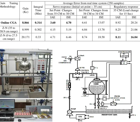
The spherical tank system exhibits non-linear behaviour due to variation on its shape. The Fig. 1, shows the experimental setup considered for modelling and analysis.The outline of the system is shown in the Fig. 2.
A. Spherical Tank System
The real time system consists of one input (inflow) and one output (level of the tank). The inflow is taken from a reservoir tank through a centrifugal pump with 3-phase motor, which is operated witha Variable Frequency Drive (VFD). The inlet pipe has a Rotameter, Orifice with Differential Pressure Transmitter (DPT) called as Flow Transmitter (FT), air-to-open type pneumatic Control Valve (CV) and a hand valve to monitor and regulate the flow rate. The orifice converts the flow into differential pressure and FT converts differential pressure into electrical signals (4 to 20 mA). The outlet has a wheel type flow meter and air-to-open type pneumatic CV to measure and regulate the outflow rate respectively. The tank level is measured using a DPT, called as Level transmitter (LT) and digital panel meters are used to monitor process and control variables. The level in the tank is directly proportional
to the pressure created by liquid in it. LT measures the bottom tank pressure with reference to the atmosphere and generates an electrical signal (4 to 20mA).
The DPTs are energized with 24V DC source and Lower Rage Value (LRV) & Upper Range Value (URV) are set using a
Highway Addressable Remote Transducer (HART)
communicator. The system is interfaced to the computer through NI USB 6211 data acquisition card (NI DAQ) and it can handle a maximum of 10 V. So, the DPT outputs (4 to 20 mA) are converted into 2 to 10V using a 500Ω resistances and scaled up using LabVIEW. The control signal (0 to 10V) from computer via NI DAQ is converted into 4 to 20 mA using a voltage to current convertor and given to current to pressure (E/P) convertor or VFD. The pneumatic line from the compressor is connected with an air regulator to obtain a constant pressure of 20 Pounds per Square Inch (PSI) and E/P converters needs this constant pressure to generate a variable pressure of 3 to 15 PSI with respect to electrical signal of 4 to 20 mA. The CVs are operated based on the pneumatic outputs from E/Ps. The VFD can vary the pump speed proportional to control signal (4 to 20 mA) and regulate the inflow rate.The description of components used in the spherical tank system is listedin Table I.
B. Process Modelling
The process modelling of spherical tank system is given by mathematical mass-balance equation (1)
) 1 ( -πR 3 4 = V = Ah = F -F 3 out in
From the equation (1), the transfer function can be determined. h. = R and R 4 = A Where, (2) -Ah 3 1 AR 3 1 F -F 2 out
in
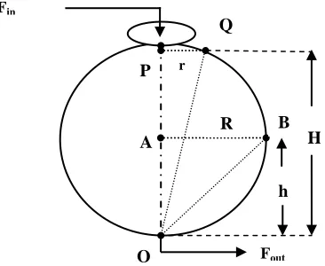
Where, Fin = input flow rate, Fout= output flow rate, A= cross sectional area, h = overall height of the tank, R = Radius of the tank, r = Variable radius with respect to Actual level of liquid.From theFig. 3, by applying side-angle-side similarity theorem ) 3 ( H rh R R r h
H
out in F F dt dh A dt
dV
R h dt dh A F , h C R h F Where V in V
out
By taking Laplace Transformation
R H(s) AsH(s) (s) F V
in
Rearranging this equation
s 1 K s AR 1 R (s) F H(s) V V
in
Where, RV = valve resistance,H= Actual level of liquid, K=RV, τ=ARV, C= valve constant, RV=
C h
The step response based open loop test is commonly adopted procedure for system identification. The process reaction curve is obtained by performing an open loop test on the real time process and model parameters are identified from the curve. LabVIEW platform is used to code the logic and the process is allowed settle at 0 cm by assigning random gain to the PI controller in closed loop and the LabVIEW Program stores flow rate with the help of FT. Now the loop is made open and flow rate is increased by P% from the stored value using LabVIEW based soft switching, which isolates the controller and the level starts increasing from 0 cm after a considerable delay called delay time. Each 400 millisecond the level is stored in a file for further analysis and it is allowed to settle through self regulation. The flow increment P% is selected therefore to make the level to reach more than half of the tank (>21.5 cm) for obtaining single mathematical model or only one set of PI parameters for the spherical tank system.
The open loop response is plotted and the values like percentage change in level from 0 to 27.5 cm (Q%), delay time (td), the time taken by the level to reach 28.3% (t1) and 63.2% (t2) are noted for getting mathematical model of the spherical tank. Two-point method is used to estimate the time constant (τ) of the system and delay time is taken directly from the response curve. The process reaction curve obtained in real time system for 0 to 27.5 cm range is shown in the Fig. 4.
τ = 1.5 (t2 - t1)
The First Order Process with Time Delay (FOPTD) model =
1 τs e K G(s) s -t P d
Maximum flow =1500 lph, and 100 lph change in flow = P% change in input.
Maximum level = 43 cm, 1% = 0.43 cm, 27.5 cm change=Q% change in output
τ =1.5 (t2 - t1) =1290 seconds
Kp= 9.593
P Q input in Change % output in Change % ) 6 ( 1 1290s 9.593e G(s) -6s
The G(s) in equation (6) is the obtained mathematical model for the entire operating range of spherical tank system
III. THE ZIEGLER-NICHOLS (Z-N) METHOD FOR PI CONTROLLER PARAMETER TUNING
The Z-N open-loop tuning method uses three process characteristics: process gain, delay time, and time constant, obtained from process reaction curve to tune the PI parameters. The controller gain (Kc) and Integral Time (Ti) are calculated using the formula given by Ziegler-Nichols. For PI control: Kc = 0.9 τ / (Kp* td);=20.171
Ti = 3.3 * td = 0.33 min
In this test the process reaction curve starts from 0 cm and ends at 27.5 cm and the PI parameters tuned from this curve is expected to providesatisfactoryvalue of the ISE and IAE when set point or load changes are given to the process for the entire operating range from 0 cm to 43 cm.
The above procedure is followed to find one more open loop response and PI controller parameters for spherical tank system, in which the initial level is maintained at 10 cm by running the process in closed loop and assigning random gain to PI controller. After level settled at 10 cm, the step change in inflow of P1% is given in open loop. In this test the process reaction curve starts from 10 cm and ends at 16.3 cm (say level change is Q1%) which is shown in the Fig. 5. The PI parameters tuned from this curve using the Z-N method is expected to provide minimum ISE and IAE when set point or load change is within the range of 10 to 16.3 cm.
Kp= 8.14
8 . 1 65 . 14 P1%
Q1%
) 7 ( 1 1065s 8.14e G(s) -5.44s
Kc= 21.411, and Ti=0.299
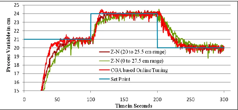
The G(s) in equation (7) is the obtained mathematical model for 10 cm to 16.3 cm range of spherical tank system From the Fig. 5, it is found that, the response of the system is more oscillatory for random PI parameters and it takes approximately 500 seconds to settle from 0 cm to 10 cm in closed loop. Now the tuned parameters are assigned to PI controller and the level of the non-linear tank is controlled in closed loop at various set points in real time when outlet valve is opened 65%. During this test, the process variable, ISE and IAE are noted at the interval of 400 milliseconds. The responses of the system, the average value of the ISE and IAE for 250 samples are compared to analyze the performance controller settings obtained from two different open loop tests, which is shown in the Fig. 6 and Table II.
The analysis shows that the model or PI controller parameters obtained in the range 10 cm to 16.3 cm performs better for positive and negative set point changes, than a single model or only one set of PI controller parameters obtained from the process reaction curve 0 to 27.5 cm range. It is concluded that multiple models and set of PI parameters are essential to improve the responses of level control process in a spherical tank at various set points or load changes.
points can be obtained. It is difficult to get 43 different open loop tests in practice and the finest responses for entire operating range are essential in industrial applications to improve product quality, productivity and safety. So the proposed method adopts an intelligent tuning method using Constrained Genetic Algorithm to get the best response in the spherical tank system.
IV. GENETIC ALGORITHMS
Genetic algorithms are random search and optimization technique based on the descriptions of natural biological evolution. GAs starts out with an initial “population” of possible solutions (individuals) to a given problem (the environment) where each individual is represented using some form of encoding called as a “chromosome”. These chromosomes are evaluated in some way for their fitness (i.e. The extent to which the individuals they represent are suitable to the environment). Using their fitness as a criterion, certain chromosomes in the population are selected for reproduction (survival of the fittest); the process of reproduction generally consists of the introduction of stochastic modifying processes such as mutation and crossover, and mechanisms by which new chromosomes can be generated.
In the proposed work, Population = group of chromosomes/solutions/individuals/parents, each chromosome in the population is a combination of two genes, Proportional Gain and Integral Time respectively.
Initial population: Each chromosome (solutions) in the population is initialized through a random process.
Evaluation: The proportional gain (gene1) and integral time (gene2) from the each chromosome are assigned to PI controller and the system responses are obtained. Maximum fitness is assigned to a chromosome, which yields better system response.
A. Selection
Selection is the stage of a genetic algorithm in which fittest individual chromosomes are chosen from a population for breeding (crossover). Tournament Selection: Tournament selection is similar to rank selection in terms of selection pressure, but it is computationally more efficient and more amenable to parallel implementation. In binary tournament selection, two chromosomes are taken at random, and the better chromosome is selected from the two by comparing the fitness values of them. In proposed work, the two chromosomes are selected for reproduction by executing the above selection process twice and the already selected ones were not replaced in the original population for the next selection.
B. Crossover
Single point crossover - The crossover point is selected between two genes and a number ‘n’ is generated through a
random process. When ‘n’ is odd, the parents’ genes from left side of crossover points are swapped or ‘n’ is even, the parents’ genes from right side of crossover points are swapped to get two offspring.
Parent 1 = {12.185 | 0.289} Parent 2 = {15.301 | 0.309}
When ‘n’ is an odd number Child 1 = {15.301 0.289} Child 2 = {13.185 0.309} (Or)
‘n’ is even number Child 1 = {13.185 0.309} Child 2 = {15.301 0.289}
C.Mutation
Mutation is a genetic operator used to preserve genetic diversity from parents to children. It alters one or more gene values in a chromosome from its initial state. Delta: First a gene of the child is chosen at random, and then that parameter (gene) is perturbed by a fixed amount, set by a delta input parameter. A gene is selected from two genes of the child through a random process with 50% probability and the selected gene is modified using delta value.
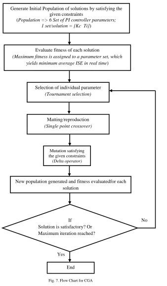
D. Constrained Genetic Algorithm (CGA)
It has all the operations of GA and constrains are assigned during mutation and initialization of the population. The sequence of operation of CGA is shown Fig. 7, in the form of flow chart
1)Constrained Initialization: During initialization, after generating each gene of the chromosome through a random process, the genes are checked to satisfy the specified constraints (lower and upper bound limits). If a gene is found to be outside the boundary limit, then it is discarded and new gene is generated randomly to satisfy the specified constraints, which leads to maintain the process variable close to set point when the CGA is operating.
2)Mutation: Delta parameter is used to modify the gene, which is selected from the child through 50% probability. After modification the lower and upper bounds are checked to avoid deviation of the process variable from set point. If the modified value is found to be, beyond the boundary limit, then it is brought to within the limit by giving suitable modification.
Let the lower and upper boundary limits of proportional gain (gene1) and integral time (gene2) are 12 and 15and Integral Time 0.2min and 0.32 min respectively.
Let the delta value gene1=0.2 and gene2 = 0.005.
↓ ↓ x y
Let the Selected gain = x
Modified gain = x-0.2 If (Modified gain < 12) then Modified gain =x+0.2
Child = {13.385 0.309} (OR) Let the Selected gain = y
Modified gain = Ti-0.005 If(Modified gain < 0.2)
then Modified gain =Ti + 0.005
Child = {13.185 0.304}
V. CGA BASED ONLINE PI CONTROLLER PARAMETER TUNING
In online method, the PI controller parameters are altereddynamically while the process is running and the performance of the parameter is analyzed based on the real time ISE. This method requires only one set of approximate PI parameter values to set the constraints when the CGA is operating, which can be obtained from Z-N open loop response and it does not require mathematical model.
Initially the parameter obtained from the Z-N method is assigned to the PI controller and required set point is given in LabVIEW. The feedback from the spherical tank is taken and connected to the controller through LT and NI DAQ. The controller controls the inflow through VFD. When the process variable reaches a nearby set point, CGA initiates operation.
The population is initialized through the constrained initialization process. In the proposed work the constraints for gene1 (Kc) is set from 8 to 16 and gene2 (Ti) is from 0.2 to 0.33. Since constraints are set, the real time response (process variable) does not deviate much from set point and minimizes the search space. One set of parameter from the populations is assigned to PI controller and tested in real time and ISE is monitored for each 400 milliseconds over a period of 30 seconds. The set of parameters (Chromosome) yields minimum average ISE for 30 seconds is assigned with maximum fitness and this chromosome influence more in the next generation. When ISE exceeds 10, then the parameters are discarded immediately, the fitness of that chromosome is assigned to zero and next set of parameter of the population is loaded. Since the chromosome with larger ISE is given minimum fitness value, the chromosome will not have any impact in the next generation. Once, all the chromosomes in the population are tested, then selection, crossover, constrained mutation operators are used to get new population and the process is repeated 6 times to get optimum solution.
Population size: 6 (6 possible set of PI parameters) Chromosome: 2 genes/ chromosome
Number of generations: 6
Crossover: single point crossover Mutation: delta operator with constraints.
Since the real time process responses are compared for performance analysis,the PI controller parameters obtained through online CGA tuning gives satisfactory responses. The intelligent is added in the process by comparing real time ISE, helps to maintain the level very close to set point, even when the PI parameters are changed during CGA operation. Based on the requirements the stopping conditions, population size and number of generations can be changed to get optimal responses.
VI. REAL TIME IMPLEMENTATION OF LEVEL CONTROL The PI controller parameters are tuned using 3 different methods, Z-N with 0 to 27.5 cm range, Z-N with specific range (Say 10 to 16.3cm), and CGA based online tuning. The servo responses of the real time system are obtained through experimental study, by assigning tuned parameters to the controller for maintaining the level of the spherical tank at various set points, 0 to 10 cm, 10 to 13 cm & 13 to 9 cm. The set point changes at every 100 seconds are given through the LabVIEW program. The real time process variable (level), ISE and IAE are stored in a file (File extension: lvm) at every 400 milliseconds for further analysis.
The regulatory response is taken through experimental study, by allowing the process variable to settle at a specified set point with 20% disturbance (outlet valve is 20% open). Now the outlet valve is opened to 100% for 15 seconds and then the valve is set to the previous level of 20% open through soft switching, then the process parameters are recorded for 100 seconds.
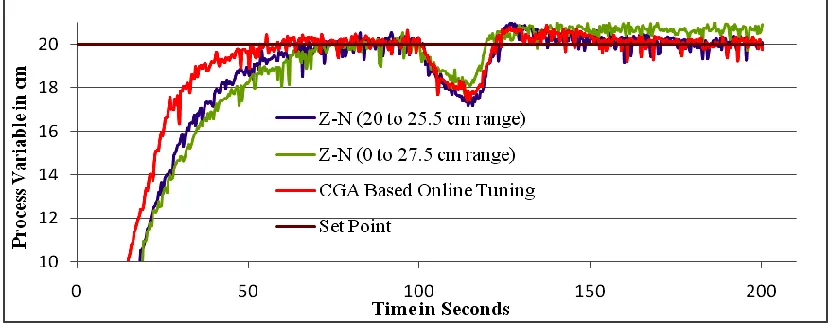
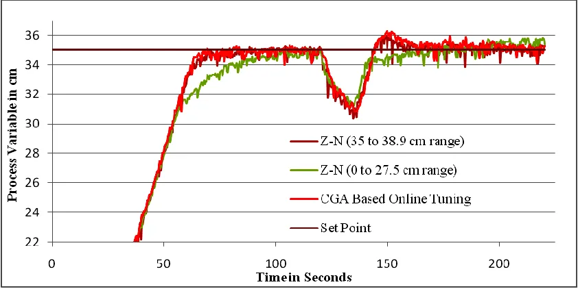
The servo and regulatory responses are obtained for all gain tuning methods separately for giving uniform step and load change and the results are consolidated for analysis. Similarly, the PI controller parameter tuning and implementation of the middle range (20 to 25.5cm) and upper range (35 to 38.9 cm) of the spherical tank are done and results are stored in different files for analysis.
VII. RESULTS AND COMPARATIVE ANALYSIS The servo and regulatory responses of the four different tuning methods are compared in terms of the performance indices such as ISA and IAE. The real time ISE and IAE values are taken from the resultant files; the average of value IAE and ISE are calculated for 250 samples and tabulated for comparison. The Table III, Shows the comparative results of the lower range of set points (9 to 13 cm). The results of middle (20 to 24 cm) and upper (34 to 38) set points are compared in Table IV, and Table V respectively.
response plots are shown in Fig. 11, Fig. 12, and Fig. 13. The CGA based online tuned parameters gives satisfactory responses both in transient and steady state periods. The response of a spherical tank system obtained at 21 cm during the operation of CGA based online tuning at run time is shown in the Fig. 14, and the process variable is oscillates only at nearest set point boundary region.
VIII. CONCLUSION
The data obtained from the experimental results shows that the proposed CGA based online tuning of PI controller parameter yields better servo and regulatory response (minimum ISE and IAE) over traditional and simulation based tuning techniques. The conventional method requires 43 different sets of PI parameters (say 1 set of parameters for 1 cm) or more to control the level at various set points from 0 to 43 cm forspherical tank having a diameter of 43 cm. It is difficult to conduct 43 numbers of open loop tests in real time for a spherical tank system to get 43 sets of PI parameters using Z-N open loop tuning method. So the 4 different sets of Z-Z-N tuned parameters provideoscillatory responses for most of the step and load changes.
Based on the performance indices analysis from Tables III, IV and V (IAE and ISE), the proposed online CGA based tuning method gives the optimized parameter values of the PI controller with minimum average of IAE and ISE for various set point and load changes when compared to conventional tuning methods. In this method, the dynamic behaviour of the real time system having good set point tracking capability when compared to other tuning methods because, the PI controller parameters are tuned at run time as per its requirement. The proposed method can be adapted for level control schemes for linear and non-linear tanks to improve productivity, product quality and safety in industries. The algorithm can be easily implemented through advanced controllers used by industries like Programmable Logic Controllers and Distributed Control Systems.
ACKNOWLEDGEMENT
I express my deep sense of gratitude and heartfelt thanks to the management of the Bannari Amman Institute of Technology for extending the required facilities in the college campus. I wish to thank all the teaching and non-teaching staff of the Department of Electronics and Instrumentation Engineering for the help rendered by them at times of need. I am thankful to All India Council for Technical Education (AICTE) for funding my project. I have used the fund to get field instruments and National Instruments Data Acquisition Cards.
Title of the Project: Automation of Level Control of Non-Linear Tanks (Spherical and Conical).
Fund Name: AICTE-Research Promotion Scheme. Fund Value: INR 8, 20, 000.00; Duration 3 Years. Reference Number: 20/AICTE/RIFD/RPS(POLICY- III)70/2012-13 Date: February 15, 2013.
REFERENCES
[1] R. Anandanatarajan, M. Chidambaram and T. Jayasingh, “Limitations of a PI controller for a first-order nonlinear process with dead time,” ISA Transactions, vol. 45, no. 2, 2006, pp. 185-199.
[2] S.P. Selvaraj and A. Nirmalkumar, “Implementation of GA Based Online PI Controller Parameter Tuning for Conical Tank Level Control,” International Journal of Applied Engineering Research, ISSN 0973-4562, vol. 9, no. 22, 2014, pp. 14319-14342.
[3] R. Anandanatarajan, M. Chidambaram and T. Jayasingh, “Design of controller using variable transformations for a nonlinear process with dead time,” ISA Transactions, vol. 44, no. 1, 2005, pp. 81-91. [4] R. Dhanalakshm and R. Vinodha, “Design of Control Schemes to
Adapt PI controller for Conical Tank Process,” International Journal of Advance Soft Comput. Appl., vol. 5, no. 3, 2013, pp. 1-20. [5] V.R. Ravi, T. Thyagarajan and G. Uma Maheshwaran, “Dynamic
Matrix Control of a Two Conical Tank Interacting Level System,” Procedia Engineering, vol. 38, 2012, pp. 2601 – 2610.
[6] N.S. Bhuvaneswari, G. Uma and T.R. Rangaswamy, “Neuro based model reference adaptive control of a conical tank level process,” Journal of Cont. and Intelligent Sys., vol. 36, no. 1, 2008, pp. 98-106. [7] P. Madhavasarma and S. Sundaram, “Model Based Tuning of a Non
Linear Spherical Tank Process with Time Delay,” Instrumentation Science and Technology, vol. 36, no. 4, 2008, pp. 420-431.
[8] S. Nithya, N. Sivakumaran,T. Balasubramanian and N. Anantharaman, “Model Based Controller Design for a Spherical Tank Process in Real Time,” International Journal of Simulation Systems, Science and Technology, vol. 9, no. 4, 2008, pp. 25-31.
[9] Ziegler, JG and Nichols, “Optimum Settings for Automatic Controller,” Transaction of ASME, vol. 64, NB 1942, pp. 759-768.
[10] G.H. Cohen, and G.A. Coon, “Theoretical Consideration of Retarded Control,” Trans. ASME, vol. 75, 1953, pp. 827–834.
[11] K.J. Astrom and T. Hagglund, “Revisiting the Ziegler–Nichols step response method for PID control,” Journal of Process Control, vol. 14, 2004, pp. 635–650.
[12] I. Pan, S. Das and A. Gupta, “Tuning of an Optimal Fuzzy PID Controller with Stochastic Algorithms for Networked Control Systems with Random Time Delay,” ISA Transactions, vol. 50, no. 1, 2011, pp. 28 – 36.
[13] W. Jie-sheng, Z. Yong and W. Wei, “Optimal Design of PI/PD Controller for Non-Minimum Phase System,” Transactions of the Institute of Measurement and Control, vol. 28, no. 1, 2006.
[14] S. Mohd Saad, hishamuddin jamaluddin and Z. Intan, M. Darus, “PID Controller Tuning Using Evolutionary Algorithms,” Wseas Transactions on Systems And Control, vol. 7, no. 4, 2012, pp. 139-149. [15] J. Zhang, J. Zhuang, H. Du and S. Wang, “Self‐ Organizing Genetic Algorithm Based Tuning of PID Controllers,” Information Sciences, vol. 179, no. 7, 2009, pp. 1007 – 1018.
[16] S.M. GirirajKumar, R. Sivasankar, T.K. Radhakrishnan, V. Dharmalingam and N. Anantharaman, “Genetic Algorithms for Level Control in a Real Time Process; Sensors and Transducers,” vol. 97, no. 10, 2008, pp. 22-33.
[17] S. Nithya, N. Sivakumaran,T. Balasubramanian and N. Anantharaman, “Design of Controller for Nonlinear Process using Soft Computing”, Instru. Science And Technology, vol. 36, 2008, pp. 437-450.
Prof. S.P.Selvaraj obtained graduation in Electronics and Instrumentation Engineering from Annamalai University and Post Graduation in Control Systems from Bharathiyar University in 2001. Obtained Research fund from AICTE in RPS scheme as a Co-PI and Published many International Journal & conference papers, He has provided a major contribution to establish center of excellence in Industrial Automation at Bannari Amman Institute of Technology, 2014. He has good industry contacts to enhance teaching-learning and research activities. Research interests: Evolutionary computation, Process Control and Automation, Control Systems.
He is the recipient of “Institution of Engineers” gold medal for the year 1989. He has about 37 Years of teaching experience.
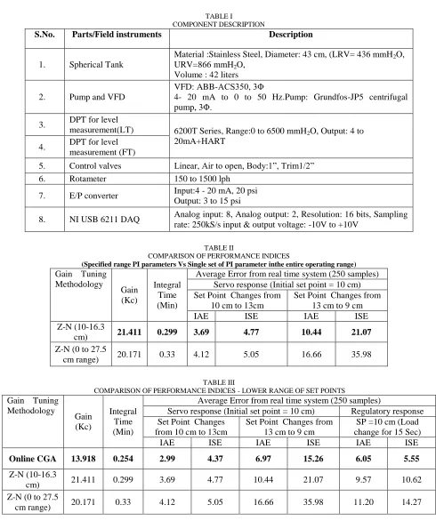
TABLE I
COMPONENT DESCRIPTION
S.No. Parts/Field instruments Description
1. Spherical Tank
Material :Stainless Steel, Diameter: 43 cm, (LRV= 436 mmH2O, URV=866 mmH2O,
Volume : 42 liters
2. Pump and VFD
VFD: ABB-ACS350, 3Φ
4- 20 mA to 0 to 50 Hz.Pump: Grundfos-JP5 centrifugal pump, 3Φ.
3. DPT for level
measurement(LT) 6200T Series, Range:0 to 6500 mmH2O, Output: 4 to 20mA+HART
4. DPT for level
measurement (FT)
5. Control valves Linear, Air to open, Body:1”, Trim1/2”
6. Rotameter 150 to 1500 lph
7. E/P converter Input:4 - 20 mA, 20 psi
Output: 3 to 15 psi
8. NI USB 6211 DAQ Analog input: 8, Analog output: 2, Resolution: 16 bits, Sampling rate: 250kS/s input & output voltage: -10V to +10V
TABLE II
COMPARISON OF PERFORMANCE INDICES
(Specified range PI parameters Vs Single set of PI parameter inthe entire operating range)
Gain Tuning Methodology
Gain (Kc)
Integral Time (Min)
Average Error from real time system (250 samples) Servo response (Initial set point = 10 cm) Set Point Changes from
10 cm to 13cm
Set Point Changes from 13 cm to 9 cm
IAE ISE IAE ISE
Z-N (10-16.3
cm) 21.411 0.299 3.69 4.77 10.44 21.07
Z-N (0 to 27.5
cm range) 20.171 0.33 4.12 5.05 16.66 35.98
TABLE III
COMPARISON OF PERFORMANCE INDICES - LOWER RANGE OF SET POINTS Gain Tuning
Methodology
Gain (Kc)
Integral Time (Min)
Average Error from real time system (250 samples)
Servo response (Initial set point = 10 cm) Regulatory response Set Point Changes
from 10 cm to 13cm
Set Point Changes from 13 cm to 9 cm
SP =10 cm (Load change for 15 Sec)
IAE ISE IAE ISE IAE ISE
Online CGA 13.918 0.254 2.99 4.37 6.97 15.26 6.05 5.55
Z-N (10-16.3
cm) 21.411 0.299 3.69 4.77 10.44 21.07 9.57 10.62
Z-N (0 to 27.5
TABLE IV
COMPARISON OF PERFORMANCE INDICES – MIDDLE RANGE OF SET POINTS
TABLE V
COMPARISON OF PERFORMANCE INDICES - HIGHER RANGE OF SET POINTS
Gain Tuning Methodology
Gain (Kc)
Integral Time (Min)
Average Error from real time system (250 samples)
Servo response (Initial set point = 35 cm) Regulatory response Set Point Changes
from 35 CM to 38 CM
Set Point Changes from 38 CM to 34 CM
35 CM (Load change for 15 Sec)
IAE ISE IAE ISE IAE ISE
Online CGA 8.866 0.314 3.60 4.70 6.61 13.07 8.92 20.24
Z-N (35 to
38.9 cm range) 8.999 0.302 4.15 5.19 6.84 13.78 8.25 21.06
Z-N (0 to 27.5
cm range) 20.171 0.33 4.71 6.46 8.74 18.58 8.11 16.04
Fig. 1. Spherical Tank Experimental Setup Fig. 2. Layout of Spherical Tank System Gain Tuning
Methodology
Gain (Kc)
Integral Time (Min)
Average Error from real time system (250 samples)
Servo response (Initial set point = 21 cm) Regulatory response Set Point Changes
from 21 CM to 24 CM
Set Point Changes from 24 CM to 20 CM
20 CM (Load change for 15 sec)
IAE ISE IAE ISE IAE ISE
Online CGA 15.101 0.228 3.36 4.97 7.11 16.32 5.46 6.84
Z-N (20 to
25.5 cm range) 13.791 0.302 3.92 6.39 8.16 18.22 6.22 8.96
Z-N (0 to 27.5
Fig. 3. Outline of a Spherical Tank
Fig. 4. Open loop Response of Spherical Tank System for 0 to 27.5 cm
Fig. 5. Open loop Response of Spherical Tank System for 10 to 16.3 cm range Fin
Fout O
R r
h H A
B P
Fig. 6. Servo Response of Spherical Tank System
Fig. 8. Servo Response of Spherical Tank System for Lower Range of Set Points
Fig. 10. Servo Response of Spherical Tank System for Higher Range of Set Points
Fig. 11. Regulatory Response of Spherical Tank System for Lower Range of Set Point
Fig. 13. Regulatory Response of Spherical Tank System for a Higher Range of Set Point
Fig. 7. Flow Chart for CGA Yes
Generate Initial Population of solutions by satisfying the given constraints
(Population => 6 Set of PI controller parameters; 1 set/solution = {Kc Ti})
Evaluate fitness of each solution
(Maximum fitness is assigned to a parameter set, which yields minimum average ISE in real time)
Selection of individual parameter
(Tournament selection)
Matting/reproduction
(Single point crossover)
Mutation satisfying the given constraints
(Delta operator)
New population generated and fitness evaluatedfor each solution
If
Solution is satisfactory? Or Maximum iteration reached?
No