Abstract—Prequalification plays a crucial role in selecting a capable contractor in construction project. Contractor prequalification studies seldom address contractor financial risk, despite the importance of contractor’s evaluation in successful project completion. Based on a cash flow based structural model using the dynamic threshold by Liao, Chen and Su, this study evaluates the credit quality of construction contractor. Via uses of the area under curve (AUC), the discriminatory performance of the cash flow model in ranking the credit qualities of construction contractors for three year is evaluated, in whichS & P issuer credit ratings are used as the benchmarks. Empirical results indicate that the proposed model has an excellent discriminatory power under AUC. Result of this study demonstrates that the proposed model is highly effective in evaluating the credit risk of construction contractors. Importantly, the proposed model only requires financial statement, making it applicable to both listed and private construction contractors.
Index Terms—Construction industry, prequalification, credit risk, cash flow.
I. INTRODUCTION
Prequalification of contractors plays a prominent role in awarding construction project. Russell and Skibniewski [1] suggested that the prequalification of contractors plays a major role in determining the success or failure of a construction project. Previous studies have suggested that prequalifying a contractor should encompass financial stability, technical ability, management capability, health and safety, as well as reputation [1], [2]. However, this information heavily relies on the subjective assessments of decision makers to identify the weights. Such information only reflects firm’s past situation under historical economic state, and it is inherently backward-looking. It is possibly incapable of assessing and forecasting the present or future credit situation.
From a cash flow perspective, contractors with adequate provision of cash or with more effective cash management ability could tolerate the adverse cash situation. However for contractors with a low consciousness priority of cash management, continuous outflow weakens their financial capability. As the cash flow of a construction contractor differs from that of other economic sectors due to the peculiarities of commercial processes in construction
Manuscript received April 22, 2013; revised June 24, 2013.
Wen-Haw Huang is with the Long Reign Development Co., Taipei (email: [email protected]).
Hui-Ping Tserng and Shu-yi Lee are with the Department of Civil Engineering of National Taiwan University (email: [email protected]; [email protected]).
Hsien-Hsing Liao is with at Department of Finance of National Taiwan University (email: [email protected]).
industry, understanding the variation of cash flow could facilitate the management of financial risk in the construction industry. However, cash flow is seldom used in previous literature as the predicting variables in the contractor prequalification. Therefore, this study assesses empirically the financial capacity of construction contractors by using a cash flow based structural model (CFB) with a dynamic threshold [3]. In particular, this study evaluates the performance of CFB with a dynamic threshold in identifying the credit level of construction contractors in the United States.
II. METHODOLOGY
Based on a CFB with a dynamic threshold, this study evaluates the credit level of construction contractors in the United State. The historical data of firms’ free cash flow is first used as the main input data of CFB with a dynamic threshold. The credit quality scores of each contractor within 3 years are then assessed by simulating the future free cash flows of contractors. Three years of performance are assessed because most construction projects are completed within three years. Additionally, effectiveness of the CFB credit model in differentiating between construction contractors as either high risk or medium/low risk is evaluated by using the receiver operating characteristics (ROC) curve.
A. CFB Credit Model
According to Liao and Chen [4], a firm’s cash flow is determined mainly by its long-term average level of cash flows, systematic state shocks, and firm specific shocks. Equation 1 established the relationship between the ith firm’s
free cash flow (Cit) at time t and the state of the economy.
1
( ) k ~ (0, 1 )
it it ij jt it it it
j
C E C α F ξ ξ N h
=
= +
∑
+ −(1) where
it
C : The ith firm’s free cash flow ij
α
: The sensitivities of the ith firm’s Cit to the jth state factor
jt
F
: The unobservable state factorsit
ξ
: The ith firm’s idiosyncratic factor representing the partof the variations of the ith firm’s C it it
h : The variance explained by the systematic factors
In this model, ith firm’s C
it is affected by a set of k
systematic factors and idiosyncratic (firm specific) effect. Unable to be explained by the state factors, the idiosyncratic factor is normally distributed with a mean of zero and a
Wen-Haw Huang, Hsien-Hsing Liao, Hui-Ping Tserng, and Shu-Yi Lee
variance equal to the residual variance not explained by the systematic factors. That is, 1- hit.
Liao and Chen [5] indicates that in most situations, a firm’s free cash flow follows a mean-reverting process, as that flow of most of the firms can be described as weakly stationary. In (1), the number of factors (k) and the factor loading
α
ij can be estimated by factor analysis.After assessing the systematic factors by using factor analysis, the model adopts a mean-reverting Gaussian process to model each state factor process for generating the paths of the future state factor. The formula of state factor process is shown as (2).
, 1
[ ]
j j j
jt F F j t F j
dF =a b −F − dt+
σ
dz(2) where
F
jtdenotes the jth state factor value at time t;j
F
a
represents the mean-reverting speed of
F
jt; jF
b
refers to the long-term average level ofF
jt;F
j t, -1denotes the jth statefactor value at time t-1; j
F
σ
refers to the standard deviation of the term variation ofF
jt, anddz
jrepresents a Wiener process. By assuming that the stochastic characteristic of the economy does not structurally change in the foreseeable future, the parameters of each state factor’s process are set as constants.Once the future free cash flows of a firm at time t are obtained, the firm asset value can be derived by discounting future cash flow. By assuming that a firm has a two-stage growth pattern in its free cash flow, the firm asset value can be obtained through (3). In the first stage, the free cash flow follows the previously developed process for the future T periods. The free cash flow is then accompanied with a constant growth rate, g, in the second stage. Therefore, for each free cash flow path, a firm’s present value Vit can be obtained at any t.
1
(1 )
(1 ) (1 ) ( )
T
i iT
it t T t
t A A A
C C g
V g τ τ τ= + γ − γ − γ ⎡ ⎤ + =⎢ + ⎥+ + −
⎣
∑
⎦ (3)In (3), Vitdenotes a firm’s present value for the ithfirm free
cash flow path at time t; Ciτrepresents the firm’s remedial cash flow for the ith free cash flow path at time t; Trefers to the
beginning time of constant growth; CiTdenotes the firm’s remedial cash flow for the ith free cash flow path at time T.
A
γ
represents the firm’s weighted average cost of capital, and
grepresents the firm’s constant growth rate after time T.
B. Default Threshold with Stationary Leverage Ratio
Duffie and Lando [5] assumed that investors lack complete information on default threshold Dt. Those investors also
formulate their default threshold assessment based on an asset value derived in previous periods. Giesecke [6] presents a structural model in which investors have incomplete information for either the firm’s asset value or the default threshold or for both. That model also assumes that investors gather more information on default threshold when a firm reaches a historical low of asset value. By following this logic,
Liao, Chen and Su (2007) set ,i.e. the upper bound of default threshold range, as historical low of the simulated asset value.
Collin-Dufresne and Goldstein [7] stated that investors believe that firms adjust their debt level Dt based on the asset
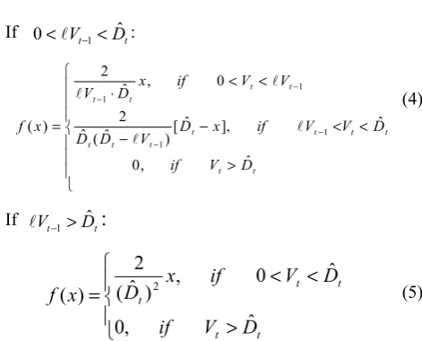
value derived in the previous period Vt-1while attempting to maintain a stationary leverage ratio. Based on this concept, Liao, Chen and Su [3] assume that investors consider the firms most likely to adjust their debt level until the current debt level divided by latest realized asset value (Dt / Vt-1) is equal to the long-term average leverage ratio(ℓ ). For simplification, Liao, Chen and Su suggest a triangular shaped distribution with probability density peaks at long-term average leverage ratio l. The probability density function of default threshold is described in (4) and (5), as shown in Fig. 1.
Fig. 1. Probability Density of Default Threshold
If 0<AVt−1<Dˆt:
t t t t t t t t t t t t t D V D V if V if x D V D D V V if x D V x f ˆ ˆ , 0 ], ˆ [ ) ˆ ( ˆ 2 0 , ˆ 2 ) ( 1 1 1 1 < ⎪ ⎪ ⎪ ⎩ ⎪ ⎪ ⎪ ⎨ ⎧ > < − − < < ⋅ = − − − − A A A A
(4)
If AVt−1>Dˆt
:
⎪ ⎩ ⎪ ⎨ ⎧ > < < = t t t t t D V if D V if x D x f ˆ , 0 ˆ 0 , ) ˆ ( 2 )
( 2 (5)
Given the derivation of an asset value path, a firm’s marginal probability of default at time t, PDt, is the area below
probability density curve within the range ( Vt-1,Vt) in Fig.1
when Vt<Vt-1 and equals zero when Vt>Vt-1.The equations are
shown in (6) and (7). In this study, PDt refers to the credit
quality score (CQSt) to more thoroughly elucidate credit
quality. If CQSt is close to 0, the contractor is either classified
as a better credit quality contractor or regarded as qualify contractor. If CQSt is close to 1, the contractor is classified as
worse credit quality contractor or regarded as a disqualified contractor.
If 0<AVt−1<Dˆt
:
⎪ ⎪ ⎪ ⎪ ⎩ ⎪⎪ ⎪ ⎪ ⎨ ⎧ > < < − − < < − = > = = − − − − t t t t t t t t t t t t t t t t t t t D V if D V V if V D D V D V V if V D V V D ob PD CQS ˆ , 0 ˆ , ) ˆ ( ˆ ) ˆ ( 0 , ) ( ˆ 1 ) .( Pr 1 1 2 1 1 2 A A A
If AVt−1>Dˆt
:
⎪ ⎪ ⎩ ⎪⎪ ⎨ ⎧
> < <
⎟ ⎟ ⎠ ⎞ ⎜ ⎜ ⎝ ⎛
− = > =
=
t t
t t
t
t t t
t
D V if
D V if D V V
D ob PD CQS
ˆ ,
0
ˆ 0 ,
ˆ 1 ) .( Pr
2
(7)
C. Model Evaluation Approach (ROC Curve)
This study also evaluates to what extent the proposed model achieves the differentiation ability in credit quality assessment. Therefore, the ROC curve is used to evaluate the extent to which the proposed model can differentiate between firms with an improved credit quality condition and those with worse credit quality condition. In contrast to the traditional evaluation method in which a single cut-off point is set, the ROC curve views every possible point as a cut-off point and, then, shows the type II error and one minus type I error accordingly. A model in which AUC=0.5 generally suggests no discrimination; with 0.7≦AUC≦0.8, it is considered an acceptable discrimination; with 0.8≦AUC≦
0.9, it is considered an excellent discrimination; with AUC≧
0.9, it is considered an outstanding discrimination (Hosmer and Leme show [8]).
III. DATA COLLECTION AND EMPIRICAL RESULTS
This study examines the credit quality of construction contractors by using the cash flow based structural model. The data is collected from the Compustat Industrial file-Quarterly data as well as CRSP (Wharton Research Data Services 2011) within the category of construction industry with the Standard Industrial Classification (SIC) code between 1,500 and 1,799. This selection criterion is the same as the one used in Severson et al. [9] and Russell and Zhai [10].
Given the restriction of collecting firms only in the construction industry, 83 construction firms were collected in 2010. However, a large number of those firms are missing quarterly operating cash flow. Moreover, the sample selection has some criteria similar to those of the cash flow based structural model, which requires a continuously free cash flow over a long term to estimate the future trend. The selection criteria are as follows:
(1) Contractors without continuously quarterly financial data are excluded.
(2) Contractors without S&P rating in the estimated period are excluded, since S&P rating is compared to the credit quality derived by the cash flow based structural model.
Following screening, the final sample consists of 22 construction contractors. Parameters of the cash flow based structural model are then estimated using continuous financial data from 2001 to 2010 (10 years data). Next, credit risk of the construction contractors is assessed.
Assessing the credit quality score:
Assessing the future credit quality score (CQS) of 22 construction contractors initially involves estimating parameters and the stimulation process. The procedures are described as follows:
Step 1. Implement a free cash flow proxy.
The quarterly financial data (2001Q1-2010Q4) of 22 construction contractors are adopted for modeling and empirical analysis because calculating parameter estimates that require a sufficient time series of data points and quarterly financial data are the most assessable source. FCFF per unit asset book value (calculated as FCFF divided by total asset book value in 2010Q4, TA) is used hereinafter to eliminate the scale effect of firms.
Step 2. Perform factor analysis and estimate the parameters of the state factor process.
Factor analysis is performed in this study to extract factors and derive the relationship between a firm’s cash flow and state factors from (1). The SPSS software is used in this study for the factor analysis. Quarterly free cash flows per unit asset (FCFF/TA) of the 22 firms are the input data for factor analysis with the estimation period from 2001Q1 to 2010Q4. Five factors are extracted with eigen values greater than unity, account for about 80.86% of free cash flow variation of these firms, as shown in Table I. Simultaneously, factor analysis generates factor loadings on the free cash flows and time-series state factor values of each firm. The time series state factor values are the inputs to maximum likelihood estimation (MLE) method to estimate the parameters of the state factor process, denoted as , and σ in (2). Table II lists the estimated parameters. With these estimated parameters, simulating 1,000 paths of each factor serves as the foundation of future state factor paths of firms. Based on each set of simulated factor paths and the factor loadings of each firm, the corresponding 1,000 future cash flow paths of each firm can be derived from (2). The simulation process and all of the calculations of the procedures are developed by using Excel software with Visual Basic programming language.
TABLEI:FACTOR EXTRACTION
Eigenvalue %of Variance Explained
Cumulative % Explained
Factor 1 9.515199 43.250907 43.250907 Factor 2 3.318260 15.083001 58.333908 Factor 3 2.190636 9.957437 68.291345 Factor 4 1.489273 6.769424 75.060769 Factor 5 1.276551 5.802504 80.863273
TABLEII:PARAMETERS ESTIMATIONS FOR STATE FACTOR PROCESS
Paramet ers
Mean-revertin g speed
Long-term average
S.D. of variation
Factor 1 0.305476 0.042297 0.793111 Factor 2 0.380616 0.042297 0.914608
Factor 3 0.830884 0.021168 1.31247
Factor 4 1.067592 0.004778 1.499048 Factor 5 0.410348 0.216035 0.990554
Step 3. Discount the future cash flow time series to forecast the future firm asset value and estimate the shift term to a firm’s cash flow paths.
A. Estimation of a Firm’s Weighted Average Cost of Capital
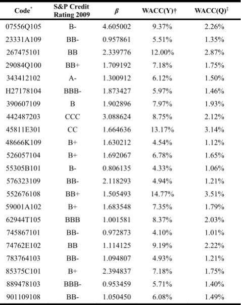
A firm’s weighted average cost of capital (WACC) consists of equity required return ( ) and cost of debt ( ), as shown in (6). A firm’s equity required return is estimated using a one-factor CAPM. Where D denotes the firm’s 2010 Q4 total liability; E represents the firm’s 2010Q4 equity book value; A refers to the firm’s 2010 Q4 total asset. The required parameters are as follows: risk free rate ( ),market risk premium ( − ) and firm’s market beta (β). The risk free rate ( ) is the 10 year U.S. treasury rate on 2010/12/31-3.98%, as obtained from the Federal Reserve Bank. The market risk premium is set at 6.70% according to Ibbotson Associates [11]. The market beta (β) of each firm is estimated as the covariance of firm’s equity return and the market over the variance of market return. The β are obtained from 5 year monthly stock data. For simplicity, a firm’s cost of debt is assumed to be a constant and equal to the market rate of the corporate bonds that have the same credit rating. Given the above information, WACC ( ) of each firm can be estimated. Tables III shows the estimated WACC.
TABLEIII:THE ESTIMATION RESULT OF EACH FIRM’S WACC
Code* S&P Credit
Rating 2009 β WACC(Y)† WACC(Q)‡
07556Q105 B- 4.605002 9.37% 2.26%
23331A109 BB- 0.957861 5.51% 1.35%
267475101 BB 2.339776 12.00% 2.87%
29084Q100 BB+ 1.709192 7.18% 1.75%
343412102 A- 1.300912 6.12% 1.50%
H27178104 BBB- 1.873427 5.97% 1.46%
390607109 B 1.902896 7.97% 1.93%
442487203 CCC 3.088624 8.75% 2.12%
45811E301 CC 1.664636 13.17% 3.14%
48666K109 B+ 1.630212 4.54% 1.12%
526057104 B+ 1.692067 6.78% 1.65%
55305B101 B- 0.806135 4.33% 1.06%
576323109 BB- 2.118293 4.94% 1.21%
552676108 BB+ 1.505493 14.77% 3.51%
59001A102 B+ 1.683548 7.35% 1.79%
62944T105 BBB 1.001581 8.37% 2.03%
745867101 BB- 0.972873 4.10% 1.01%
74762E102 BB 1.114125 9.19% 2.22%
783764103 BB- 1.094807 4.93% 1.21%
85375C101 B+ 2.394837 7.18% 1.75%
889478103 BBB- 0.953459 5.71% 1.40%
901109108 BB- 1.050450 6.08% 1.49%
B. Estimation of Constant Growth Rate
This study follows the assumption of Liao and Chen [4], in which a firm grows at a constant rate after 10 years from the pricing time. Namely, T is set as 10 in (3). A firm starts with constant growth at the beginning of 10 years. For simplicity, the average of 10-year U.S. GDP growth rate 0.3874 (quarterly) is proxy for a firm’s constant growth rate, which is obtained from Federal Reserve Bank.
C. Estimation of the Shift Term to a Firm’s Cash Flow Paths
As is well known, the asset values in the first period may
vary from path to path and apart from the present market asset value. Therefore, the calibration step adjusts a firm’s present value of the future free cash flows at the same points, which is the current market asset value. After adding back a shift term (m) in each simulated cash flow path, the adjusted simulated cash flow paths match the market value. Notably, the adding back of shift term does not change the correlation structure and volatility characteristic of the cash flow paths. Table IV summarizes those results.
TABLEIV:SHIFT TERM AND LONG-TERM AVERAGE LEVERAGE RATIO
Code* Implied Cash Flow Shift Term† Long-termAverage Leverage Ratio†
07556Q105 0.02519 64%
23331A109 -0.06995 17%
267475101 -0.16549 24%
29084Q100 -0.05782 25%
343412102 -0.08699 34%
H27178104 -0.05698 65%
390607109 -0.08113 93%
442487203 -0.00395 71%
45811E301 -0.03342 82%
48666K109 -0.04249 57%
526057104 -0.03225 58%
55305B101 -0.02353 42%
576323109 -0.06127 81%
552676108 -0.02432 45%
59001A102 -0.01123 87%
62944T105 -0.18540 13%
745867101 -0.04353 54%
74762E102 -0.07129 62%
783764103 -0.02551 48%
85375C101 -0.03721 46%
889478103 0.01444 48%
901109108 -0.02143 61%
Step 4. Utilize the dynamic default threshold with stationary leverage ratio.
The long-term leverage ratio (ℓ) for each firm is evaluated with financial information from 2001Q1 to 2010Q4.The ratio of the book value of debt to the sum of book value of debt and market value of equity are the proxy for leverage ratio. Market value of equity equals the stock price multiplied by outstanding equity shares. The data are collected from the COMPUSTST database. Table IV summarizes the long-term average ratio results. After the leverage ratio and default threshold are set, the CQS of each firm at any time t can be calculated by (6) and (7) with 1,000 simulated adjusted firm value paths.
Credit Quality Score and Model Discriminatory Power: With simulation and parameters estimation, the credit quality scores of each firm at every t period can be obtained. Long-term performance of the proposed model is assessed by evaluating the firm’s credit quality scores in 1-year, 2-year and 3-year (Table V).
to meet financial obligations) to SD (selected default). In this study, a firm with a rating higher or equal to BBB is known as investment grade, whereas a firm’s rating below BBB is considered speculative grade. Therefore, based on the Area Under Curve (AUC) assessment criteria, this study evaluates the model discriminatory power between investment and speculative grade.
The AUC results of model in 1-year are 0.8611; 2-year is 0.8333; and 3-year is 0.8194.
TABLEV:CREDIT QUALITY SCORE
Code* Rating 2011 S&P Credit Year Year Year
07556Q105 B- 0.023973 0.058117 0.087973 23331A109 BB- 0.036922 0.069484 0.091817 267475101 BB 0.005414 0.006811 0.020313
29084Q100 BB+ 0.001820 0.001926 0.003174 343412102 A- 0.002590 0.003145 0.004342 H27178104 BBB- 0.001643 0.001961 0.003357 390607109 B 0.051796 0.065093 0.112568 442487203 CCC 0.016404 0.030066 0.062276 45811E301 CC 0.030949 0.056664 0.083805 48666K109 B+ 0.011563 0.019102 0.047116 526057104 B+ 0.016602 0.047504 0.055119 55305B101 B- 0.024439 0.067662 0.096082 576323109 BB- 0.194006 0.237980 0.267509
552676108 BB+ 0.000755 0.000751 0.00091 59001A102 B+ 0.058006 0.107361 0.154975 62944T105 BBB 0.004363 0.005873 0.014316 745867101 BB- 0.034835 0.068183 0.096924 74762E102 BB 0.001963 0.001915 0.002717 783764103 BB- 0.019687 0.053788 0.083328 85375C101 B+ 0.065777 0.098407 0.149882 889478103 BBB- 0.003631 0.006429 0.011971 901109108 BB- 0.007247 0.011428 0.012414
IV. CONCLUSION
Prequalification of construction contractor plays a critical role in construction risk management. As the cash flow of a construction contractor mainly reflects its financial ability, this study investigates the prequalification of construction contractor from a financial perspective. The contractors’ credit risk is then assessed by using CFB with a dynamic threshold. Next, based on use of S&P issuer credit ratings as the benchmarks, the model’s discrimination power is evaluated to differentiate high risk from medium/low risk. Empirical results indicate that the CFB with a dynamic threshold achieves an excellent discriminatory ability in assessing the credit risk of construction contractors in the United States.
This study has several implications. First, CFB with a dynamic threshold is applicable to construction contractors in the United States. Second, CFB with a dynamic threshold requires only quantitative information in modeling to avoid a bias in human judgment. Third, CFB with a dynamic threshold attains a long-term stable performance within the duration of a construction project period, mainly in two to
three years.
REFERENCES
[1] J. S. Russell and M. J. Skibniewski, “Decision criteria in contractor prequalification,” Journal of Management in Engineering, vol. 4, no. 2, pp. 148-164, 1988.
[2] A. Merna and N. J. Smith, “Bid evaluation for UK public sector construction contractors,” in Proc. The Institution of Civil Engineers, vol. 1, no. 88, pp. 91-105, 1990.
[3] H.-H. Liao, T.-K. Chen, and Y. H. Su, “Credit analysis of corporate credit portfolio─A cash flow based conditional independent default approach,” presented at The Asian Finance Association 2009 International Conference, Brisbane, Australia, June 30–July 3. [4] H.-H. Liao and T.-K. Chen, “A cash flow based multi-period corporate
credit model,” SSRN eLibrary (2004). [Online]. Available: http://ssrn.com/abstract=753304 [cited 1 March 2011]
[5] D. Duffie, and D. Lando, “Term structures of credit spreads with incomplete accounting information,” Econometrica, vol. 69, pp. 633-644, 2001.
[6] K. Giesecke, “Correlated default with incomplete information,” Journal of Banking and Finance, vol. 28, pp. 1521-1545, 2004. [7] P. Collin-Dufresne and R.S. Goldstein, “Do credit spreads reflect
stationary leverage ratios,” Journal of Finance, vol. 56, pp. 1929-1957, 2001.
[8] D. W. Hosmer and S. Lemeshow, Applied Logistic Regression, John Wiley & Sons, Inc., New York, 2000.
[9] G. D. Severson, J. S. Russell, and E. J. Jaselskis, “Predicting contract surety bond claims using contractor financial data,” Journal of Construction Engineering and Management, vol. 120, no. 2, pp. 405-420, 1994.
[10] J. S. Russel land H. M. Zhai, “Predicting contractor failure using stochastic dynamics of economic and financial variables,” Journal of Construction Engineering and Management, vol. 122, no. 2, pp. 183-191, 1996.
[11] Ibbotson Associates, Stocks, Bonds, Bills and Inflation, Ibbotson Associates, annual, 2011.
Wen-Haw Huang is a general manager of the Long Reign Development Co., a real estate company in Taipei. Currently, he is a Ph.D. Student in the Department of Civil Engineering at National Taiwan University. His research interests are construction finance, construction management, and project performance evaluation.
Hui-Ping Tserng is a professor at the Department of Civil Engineering of National Taiwan University. He has a Ph.D degree in Construction Engineering and Management from University of Wisconsin-Madison and he is an official reviewer or editorial board member of several international journals. His research interests include advanced techniques for project management, construction finance, knowledge management, management information system, GPS/Wireless Sensor Network, and automation in construction.
Hsien-Hsing Liao is a professor at Department of Finance of National Taiwan University. He has a Ph.D. degree in Rutgers University. His research fields are speculative Bubbles in Real Estate Market, Risk Factors in Real Estate Market, Information Content of Real Estate Related Information.
Shu-yi Lee received her bachelor and master degree from the Department of Civil Engineering of National Taiwan University. She is now working as research assistance in the Department of Civil Engineering of National Taiwan University.