Parallel Performance of Domain Decomposition Method on Distributed Computing Environment

(1)

IACSIT International Journal of Engineering and Technology Vol. 2, No.1, February, 2010 ISSN: 1793-8236

28 1

Abstract— Distributed parallel computing, which uses general- purpose workstations connected by a network as a large parallel computing resource, is one of the most promising trends in parallel computing. Over the last two decades, the growth in the use of such parallel computing environment has ensured the interest on the parallel finite element method. In this work, parallel finite element method using domain decomposition technique has been adapted to the distributed parallel environment of networked workstations and the supercomputer. Using the developed parallel code, two model problems are solved and the parallel performances are analyzed on the network of eight Pentium IV PC cluster and GP7000F workstations. The models are High Temperature Test Reactor and Advanced Boiler Water Reactor. The later model with very large size, over 11 million degrees of freedom has been solved using 1024 SR8000 supercomputer. We have tested the numerical and parallel scalable properties of the domain decomposition method with employing suitable preconditioners. The result shows that the method is numerically scalable and efficient in parallel processors.

Index Terms— Domain decomposition, finite element, parallel computing, workstation cluster.

I. INTRODUCTION

Large scale problem, particularly those defined in three dimensional domain, often need substantial computation time and memory to run on ordinary sequential computers. Even if they can be solved, powerful computation capability is required to obtain the accurate and precise results within a reasonable time. Parallel computing can meet requirements of high performance computation [1]. Among the various parallel computing algorithms, Domain Decomposition Method (DDM) has become much popularity in the recent years [2]. In this method, the whole domain to be solved is first decomposed into a number of subdomains without overlapping. Finite Element Analysis (FEA) is defined and solved in each subdomain in parallel and then partial solutions are assembled together to get the global solution.

This method is exclusively implemented on structural analysis [3], heat conduction problem [4] and fluid analysis [5]. Most of the papers emphasizes only on the implementation of the method without analyzing the parallel performance as well as taking the necessary advantages of the parallel computing environment. In this research, the two

Manuscript received November 11, 2009

A. M. M. Mukaddes is with department of Industrial and Production Engineering, Shahjalal University of Science and Technology, Sylhet, Bangladesh (email: [email protected]).

Ryuji Shioya is with Toyo University, Japan

parallel approaches (dynamic load distribution [6] and static load distribution) of domain decomposition method with a suitable preconditioner have been adapted to the distributed parallel environment of networked workstations [7] and the supercomputer. The scalability of the preconditioners has been evaluated in the parallel computers.

Using the developed code several models are solved and the performances are measured in different computing environments. The important factors affecting the performance of parallel computing using the domain decomposition method are found and analyzed. This analysis will be useful as a guideline for the user of the domain decomposition based software in the parallel computing environment.

II. DOMAIN DECOMPOSITION METHOD Main method:

Consider a linear system of algebraic equations,

[ ]

K

{ } { }

u

=

f

(1) arising from a finite element discretization of a linear elliptic

boundary value problem in the domain

Ω

,

where

K

is the global stiffness matrix,

u

is an unknown vector and

f

is a known vector. The domain

Ω

to be solved is first decomposed into N number of subdomains,

{ }

( )

N ,..., i i

1 =

Ω

as shown in Fig. 1, for which the union of all subdomains boundaries is

( )

U

_iN i

_.

1 =

Γ

=

Γ

(2) Let

u

(i)be the vector corresponding to the variables in

) (i

Ω

, and let R(i) be the 0-1 matrix that maps the degrees of freedom

u

(i)into global degrees of freedom. R(i)Tis the transpose of R(i), then

u

(i)

=

R

(i)T

u

and by the standard subassembly process,

Parallel Performance of Domain Decomposition

Method on Distributed Computing Environment

(2)

29

Fig. 1 Partition of non-overlapping subdomains

Fig. 2 Action of

R

_B( )iT

∑

= = N i T i i i _K _R

R K 1 ) ( ) ( )

( ₍₃₎

where

K

( )i be the local stiffness matrix corresponding to

subdomain

Ω

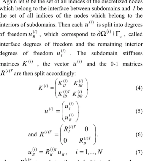
(i)

Again letBbe the set of all indices of the discretized nodes which belong to the interface between subdomains and Ibe the set of all indices of the nodes which belong to the interiors of subdomains. Then each

u

(i) is split into degrees of freedom

u

_B(i) , which correspond to

∂

Ω

( )i

\

Γ

_u , called interface degrees of freedom and the remaining interior degrees of freedom

u

(_Ii) . The subdomain stiffness matrices

K

(i) , the vector

u

(i) and the 0-1 matrices

T i

R

() _{are then split accordingly:}

, ) ( ) ( ) ( ) ( ) ( ⎟ ⎟ ⎠ ⎞ ⎜ ⎜ ⎝ ⎛ = _i BB T i IB i IB i II i K K K K

K (4)

,

) ( ) ( ) (

⎟

⎠

⎞

⎜

⎝

⎛

=

_i B i I i

u

(5)

and

_⎟

⎟

⎠

⎞

⎜

⎝

⎛

=

_i_T

B T i I T i

R

) ( ) ( ) (

0

. (6)

( )

_R

( )

_u

_,

_i

_,...,

_N

u

iT _B

B i

B

=

1

(7)

where

( )iT B

R

translates the global interface nodes

to local interface numbering as shown in fig. 2 .

Let

V

( )i be the space of the interface degrees of freedom for

the subdomain

Ω

( )i and

V

denotes the space of all degrees of freedom on

Γ

.

The unknown in the interior of the

subdomain

Ω

( )i is eliminated by Gaussian elimination according to the equation (8) using an initial value of

u

B( )i ,

( ) ( )

(

( ) ( ) ( )i

)

B i IB i I i II i

I

K

f

K

u

=

−1

−

_{. (8)} Then, after elimination of the interior degrees of freedom,

the problem (1) reduces to a problem on the interface space

V

,

g

Su

_B

=

(9) where

S

is the Schur complement matrix:

( ) ( ) ( )

∑

=

N_i iT B i i B

S

R

S

₁ , (10)

( ) ( ) ( )

( )

( ) ( )i IB i II T i IB i BB

i

_K

S

=

−

−1 . (11) The problem (9) is solved using the preconditioned

conjugate gradient method.

Again it is important to remember that if

Ω

( )i is an interior subdomain (floating subdomain), then

S

( )i is a singular matrix. We must therefore apply a pseudoinverse or a generalized inverse. We choose a generalized inverse that uses a small regularization parameter

α

, replacing problems with

S

( )i by non-singular problems with

( )₊

[

( )

{

( )

}

]

−1

α

+

=

S

max

diag

K

I

S

i

BB i

i _{, (12)}

where the

max

{

diag

( )

K

_BB( )i

}

is the maximum value of diagonal elements of matrix

K

(_BBi) and I is the identity matrix.

Preconditioners [8]:

The present domain decomposition method includes the following preconditioning techniques [8]

Simplified diagonal scaling:

( )

(

)

∑

=

−

=

_iN iT

B i BB i

B

DIAG

R

diag

K

R

Q

₁ () () 1 () ₍₁₃₎

Balancing domain decomposition (BDD): This preconditioning matrix is defined as

(

c

) (

l c

)

c

BDD

Q

I

Q

S

Q

I

SQ

M

−1

=

+

−

₍₁₄₎

where

Q

_l is the local level part and

Q

_c is the coarse level part of the preconditioner.

Balancing domain decomposition with diagonal scaling:

DIAG c

DIAG

BDD

I

Q

S

Q

M

−1

₌

(

₋

)

− (15) Incomplete balancing domain decomposition (IBDD):

(

c

) (

l c

)

c

IBDD Q I Q S Q I SQ

M−1 = ~ + −~ − ~ ₍₁₆₎

where Q~_c is constructed from the incomplete factorized coarse operator

Incomplete balancing domain decomposition with simplified diagonal scaling (IBDD-DIAG):

(

c

)

DIAG

(

c

)

c DIAG

IBDD Q I Q S Q I SQ

M−1 ₌ ~ ₊ ₋ ~ ₋ ~

− (17)

III. PARALLELISM OF THE DOMAIN DECOMPOSITION

METHOD

(3)

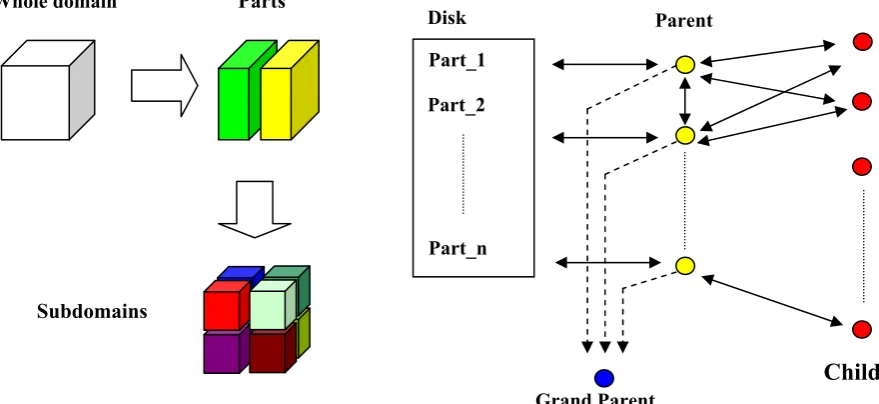
30 which are further decomposed into smaller subdomains. In this research we adopt Hierarchical Domain Decomposition Method (HDDM) [6] which is a well known parallel DDM. This hierarchically structured DDM classifies processors in two different following ways.

Dynamic load distribution (h-mode):

The h-mode classifies processors into 3 groups, ‘Grand Parent’, ‘Parent’ and ‘Child’. Fig. 3 illustrates the practical implementation of hierarchical organized processors in the present method. One of the processors is assigned as Grand Parent, a few as Parent, and others as Child. The number of processors assigned as Parent is the same as that of parts. The number of Child processors can be varied; and it affects the parallel performance.

The role of Grand Parent is to organize all processor communications (i.e. message passing) which occur between all processors.

Parents prepare mesh data, manage FEA (Finite Element Analysis) results, and coordinate the CG iteration, including convergence decision for the CG iteration.

Parents send data to Child processors, where FEA is performed in parallel. After the FEA, Child processors send

the results to Parents. This computation will be repeated until the CG iteration is convergent.

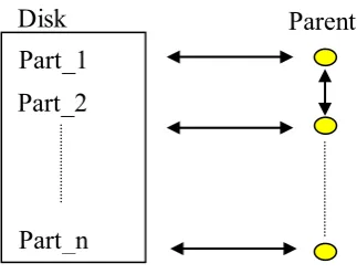
Static load distribution (p-mode):

However, because almost all computation is performed in Child processors and the most communication time is taken between Parent processors and Child processors, so the communication speed becomes important. In recent years although the communication performance has also been improving by improvement in network technology, the high-speed network is still expensive. On the other hand, for the PC cluster generally used, the network speed becomes a bottleneck to the processing performance of CPU. Moreover, when a parallel processing performance is considered, it is important to reduce the amount of communication time as much as possible. Therefore, the Parent-Only type (static load distribution: p-mode) is useful than the conventional Grand-Parent-Child type (h-mode).

Fig. 4 shows the parallel processor scheme of p-mode. In the p-mode, the Parent processors perform the FEA by themselves, which is computed by the Child processors in the h-mode. In the h-mode, although Parent processors store some of the subdomain analysis data and coordinate the CG iteration as the main work, the idling time of CPU increases because of less computation in Parent processors.

Fig. 3 Hierarchical domain decomposition method (left), dynamic load distribution (right)

Whole domain Parts

Subdomains

Disk

Part_1

Part_n Part_2

Parent

Grand Parent

(4)

31

Disk

Part_1

Part_n

Part_2

Parent

Fig. 4 Parallel processor scheme (p-mode)

On the other hand, in the p-mode, since all processors perform the FEA and CPU can be used without futility, in uniform processor’s environment, p-mode is considered to be predominance to h-mode. In the p-mode also, the number of Parent processors should be equal to the number of parts.

IV. PARALLEL PERFORMANCE Speed up:

The key issue in the parallel processing in a single application is the speed up achieved, specially its dependence on the number of processors used. For simplicity speed up with

n

processors,

S

n is defined as follows:

( )

A

t

A

t

S

n

=

1 (18)

where

t

₁

( )

A

and

t

_n

( )

A

are total time for solving the problem using one processor and

n

processors, respectively. Also scaled speed up

S

_n

′

is defined as follows:

( )

nA

t

A

t

n

S

n

n 1

×

=

′

(19)

where

t

_n

( )

nA

is the total time for solving the problem of size

nA

.

Sequential processing and parallel processing:

The program might be sequential, parallel or combination of sequential and parallel. The execution time to solve a problem of size

n

having the sequential processing is given by the equation (20)

( )

n T

( )

n T

( )

n

T = _calc + _i_/_o (20) where

T

( )

n

,

T

_calc

( )

n

,

T

_i_/_o

( )

n

are the total execution

time, calculation time and input/output time. Again the execution time to solve a problem of size

n

, having the parallel processing also is given by the equation (21)

( )

n p T

( )

n p T

( )

n p T

( )

n p

T , = _calc , + _i_/_o , + _comm , (21) where

T

( )

n

,

p

,

T

_calc

( )

n

,

p

,

T

_i_/_o

( )

n

,

p

and

T

_comm

( )

n

,

p

are the execution time, calculation time input/output time and time for communication respectively.

The ratio of the calculation time, input/output time and communication time over the total execution time is defined as follows

( )

n p T

p n T R_calc calc

, ) , (

= ,

) , (

) , ( / / T_T _nn_pp

R_i _o= i o ,

) , (

p n T

R_comm= comm (22)

and

1

/ + =

+ i o comm calc R R

R (23)

V. NUMERICAL RESULTS AND DISCUSSIONS

A. Physical model and computational environment:

Using the developed code, two heat transfer models [4] are analyzed here. Models are High Temperature Test Reactor (HTTR) and Advanced Boiling Water Reactor (ABWR) which are shown in fig. 5. The calculations are performed in three different computational environments shown in Table 1 and the model descriptions are shown in Table 2.

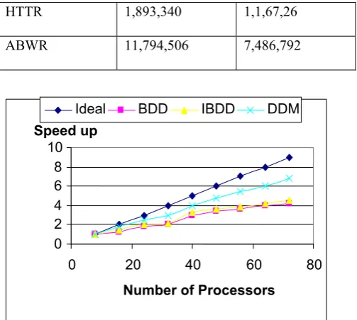
B. Scalability and speed-up:

We evaluate the parallel scalability of the BDD and IBDD-DIAG preconditioner, varying the number of processors employed. Such evaluation is performed using the HITACHI SR8000. Fig. 6 reports that BDD and IBDD-DIAG can compute faster solutions of a fixed mesh problem when the number of processors is increased. The speed-up is compared with the number of processors, referring the value for using 8 processors in Fig. 7 while the scaled speed-up with different number of processors refereeing the value of using 8 processors in Fig. 8. The results shown in Fig. 6 confirm the parallel scalability properties of the BDD and IBDD-DIAG preconditioners. Since the program has both parallelable and nonparallelable portion, results are too far from the ideal one. For the parallelable portion, parallel computing with n processors can shorten computation time to 1/n in ideal.

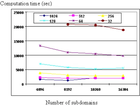
C. Results concerning the number of subdomains:

The number of subdomains is the major concern in the domain decomposition method. We compare the computation time (for IBDD-DIAG) in two different computational environments corresponding to the number of subdomains and results are shown in Fig. 9. CM shows better

Fig. 5 Part decomposition of HTTR and ABWR model

(5)

32 Fig. 10 (p-mode) and Fig. 10 (h-mode). In p-mode with the increase of number of subdomains, ratio of calculation time decreases while ratio of input/output time and communication time increases. Since the network speed of GP7000F is faster than the CM, the communication takes less time compared to the CM clustures. The Fig. 11 shows the computation time for h-mode in two different computation environments, which shows that when the number of subdomain is 3000 the computation time increases in CM cluster compared to the GP7000F. This is because, in the h-mode the more communication takes place between the Parents and Childs as the number of subdomains increases thereby in CM it takes more time for the communication. So in the parallel computing environment having low performance it is better to use the static load distribution mode and having high performance it is better to use the dynamic load distribution mode. From Fig. 9 and 11 it can be recognized the optimum number of subdomains for two computational environments for both h-mode and p-mode.

ABWR model is analyzed in the vector type supercomputer SR8000 changing number of processors. Fig. 13 (p-mode) and Fig. 14 (h-mode) shows the variation of the computation time using the different number of processors in SR8000. As the number processor increases, the difference decreases. As a result, the difference between the time required using 512 processors and 1024 processors is too small. So it is not necessary to use more than 1024 processors for this model.

Fig. 6 Computation time in different number of processors

TABLE 1PARALLEL COMPUTATIONAL ENVIRONMENTS

CPU Memory Network

PC Cluster Pentium4,

2.0GHz 1GB/CPU Ethernet (100Mbp)

GP7000F SPARC64 ,

333MHz

1GB/CPU Ethernet (1Gbps) Hitachi

SR8000

250 MHz 1 GB/CPU

TABLE 2MODEL DESCRIPTION

Model Number of Nodes Number of

Elements

HTTR 1,893,340 1,1,67,26

ABWR 11,794,506 7,486,792

Fig. 7 speed up for different number of processors ( HTTR model)

Fig. 8 Scaled speed up for different number of processors ( HTTR model)

Fig. 9 Computation time in two different computational environments (p-mode)

0 2 4 6 8 10

0 20 40 60 80

Number of Processors Speed up

Ideal BDD IBDD DDM

0 2 4 6 8 10

0 20 40 60 80

Number of processors Scaled speed up

Ideal BDD IBDD-DIAG DDM

0 500 1000 1500 2000

0 2 4 6 8

Number of processors Computation time (sec

(6)

33

Fig. 10 Ratio of calculation, input/output and communication time (p-mode)

Fig. 11 Execution time in two different computational environments (h-mode)

Fig. 12 Ratio of calculation, input/output and communication time (h-mode)

Fig. 13 Computation time vs number of subdomains in different number of processors (p-mode)

Fig. 14 Computation time vs number of subdomains in different number of processors (h-mode)

Number of subdomains

N

um

ber

o

f

iter

at

io

ns

Fig. 15 Numerical scalability of BDD type preconditioners (p-mode)

α

(7)

34

α

Fig. 17 Effect of

α

on the computation time (sec)

D. Numerical scalability:

The numerical scalability has been evaluated for the preconditioners discussed in the section II. Fig. 15 shows the number of subdomains vs the number of iterations for this analysis. The number of iterations increases with the increase of the number subdomains for the case of simplified diagonal scaling (DIAG) while the number of iterations remains constant with the number of subdomains in the case of BDD type preconditioners. So these results demonstrate that the domain decomposition method with the BDD type preconditioners is numerically scalable.

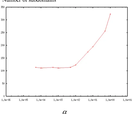
E. Effect of

α

The HTTR model is analyzed with the BDD preconditioner by changing the values of

α

in (12) to see its effect on the number of subdomains. Fig. 16 shows the number of iterations of the PCG method with the BDD preconditioner when the parameter

α

is varied. The effect of

α

on the computation time is shown in Fig. 17. When the parameter

α

is set to be less than 1.0e-3_{, the PCG}

method obtains a good convergence rate with the good performance. So, the optimum value of

α

is taken as 1.0e-3 _.

VI. CONCLUSION

Two parallel approaches, static load distribution and dynamic load distribution of the domain decomposition method are adapted to the parallel computing environment and their parallel performances are analyzed. Static load distribution seems to be more efficient in the parallel computer having low network speed while dynamic load distribution shows good performance in the high speed networked parallel computers. By the performance test, the effectiveness of the domain decomposition method in the parallel computer is verified. Important factors affecting the performance of the distributed parallel computing are found and analyzed. By using workstation cluster, a huge size of problem having over 11 million degrees of freedom is solved successfully.

REFERENCES

[1] Almasi G S and Gottlieb A, Highly parallel computing [M]. The Benjamin/Cummings Publishing Company, Inc., Redwood City, Ca, 1990

[2] Farhat, C., Chen, P.S. and Mandel, J., A scalable lagrange multiplier based domain decomposition method for time-dependent problems,

International Journal for Numerical Methods in Engineering, Vol. 38 , p. 3831-3853, 1995

[3] Shioya, R., Ogino, M., Kanayama, H. and Tagami, D., Large scale finite element analysis with a balancing domain decomposition method, Key Eng. Mate., 243-244 , p.21-26,2003.

[4] A.M..M..Mukaddes, M. Ogino, H. Kanayama and R. Shioya, A scalable balancing domain decomposition based preconditioner for large scale heat transfer problems. JSME International Journal, Series B, vol 49, No. 2 pp-533-540, 2006

[5] Kanayama, H., Ogino, M., Takesue, N and A.M.M.Mukaddes, Finite element analysis for stationary incompressible viscous flows using balancing domain decomposition, Theoretical and Applied Mechanics,

54, p.211-219, 2005.

[6] Yagawa, G. and Shioya, R., Parallel finite elements on a massively parallel computer with domain decomposition, Computing Systems in Engineering 4:4-6 , p.495-503, 1993.

[7] Kim S J, Kim J H. Large-scale structural analysis using domain decomposition method on distributed parallel computing environment. Proceedings of High-Performance Computing in the Information Superhighway. HPC-Asia, 573-678,1997.