Developing a 3D CFD Code to Simulate Incompressible Simultaneous Two-Phase Flow through a Horizontal Bend Using VOF Principle



Abstract—Most hydrocarbons production systems inevitably operate under multiphase flow conditions. While there is an agreement that Navier-Stokes equations govern variables for single-phase flow; there is no such consensus for the multiphase flow yet.

Different numerical methods with dissimilar concepts are being conveniently used to simulate multiphase flow systems. Some of these methods do not respect the balance while others damp down strong gradients. The degree of complexity of these models makes the solution practically not reachable by numerical computations despite the fact that many rigorous and systematic studies have been undertaken so far. The essential difficulty is to describe the turbulent interfacial geometry between the multiple phases and take into account steep gradients of the variables across the interface in order to determine the mass, momentum and energy transfers.

Different numerical techniques have been developed to simulate the gas-liquid simultaneous flow utilizing the CFD (Computational Fluid Dynamics) discipline. For example, the Volume of Fluid (VOF) model, the Eulerian-Langrangian models and the Eulerian-Eulerian models and combinations between these models.

This paper presents the outcomes of numerical investigation carried out to probe the effect of a horizontal bend on the behavioral phenomenon of incompressible air-water simultaneous flow. A 3D CFD code has been developed based on NASA VOF code, which was designed for a different application. Major modifications were implemented on the original program to develop a fit-for-purpose one. The results have been qualified with the experimental data available from a different part of the same project and satisfactory agreements were obtained.

Index Terms—CFD, VOF, incompressible multiphase flow, horizontal bends, pressure drop, velocity profile.

I. INTRODUCTION

Numerous number of techniques available in the literatures for the numerical simulation of two-phase flows. In general, these techniques could be classified under two main categories:

A. Correlations and Analytical Approaches

These approaches provide predictive means to establish the features of two-phase flow through formulating correlations from experimental data. Although correlations may be complex and incorporate many variables, they are generally limited to use with systems that are similar to those used to provide the data for their construction. In this

 Manuscript received June 14, 2016; revised October 10, 2016. Amir Alwazzan is with Dragon Oil Ltd., Dubai, UAE (e-mail: [email protected])

respect, it would be far from satisfactory to describe the features of a two-phase flow analytically. Generally though, gross simplification of the governing equations is necessary for a complete analytical solution to be possible. In this case, closure relationships are necessary which relate phase interaction and these have to be established on an empirical basis.

B. Numerical Modeling of the Free Surfaces

Several numerical methods have been designed and developed to describe time-dependent flows of multiple immiscible fluids. These flows are characterized by the presence of interface between phases, which divide the flow domain into regions of individual component fluids. The interface may be identified to be a demarcation surface across which steep changes (or discontinuities) in fluid properties exist. The free surface may be an extreme form of such interfaces in which the density of one fluid (gas) is negligibly small in comparison to the other fluid (liquid).

Where the phases are completely separated, as in the stratified and annular flows, the effect of the interfaces position becomes significant and analytical methods are usually unable to provide adequate solution.

The method of Volume of Fluid (VOF) was suggested by Nichols et al. [11] and Hirt & Nichols [5]. They defined the function F, whose value is unity at any point occupied by fluid and zero otherwise. VOF specifies that a free surface cell is identified as one, which has a fractional volume between zero and one. The conservation equations for the field variables are solved by using an advection scheme on an arbitrary Lagrangian-Eulerian mesh. Fluids’ interface is traced by tracking the sharp variation of the fluid volume fraction. This approach is capable of depicting the interface with a minimum requirement of storage.

Torrey et al. [14] presented a two dimensional, transient free surfaces hydrodynamics program (NASA-VOF 2D). This program is based on the VOF method and it allows multiple free surfaces with surface tension and wall adhesion. It also has a partial cell treatment that allows curved boundaries and internal obstacles. Torrey et al. [15] developed the NASA-VOF 3D code based on NASA-VOF 2D [14] and SOLA-VOF code [11]. NASA-VOF 3D has been designed to calculate confined flows in a low gas environment including multiple free surfaces with surface tension and wall adhesion. It also has the capability to address partial cell treatment that allows curved boundaries and internal obstacles.

Kwak & Kuwahara [8] presented a new scheme for the VOF method by including the cross directional upstream effects. This advection scheme is interlinked with the Flux Corrected Transport (FCT) technique to guarantee the

Developing a 3D CFD Code to Simulate Incompressible

Simultaneous Two-Phase Flow through a Horizontal Bend

Using VOF Principle

monotonicity in the solution. Together with the interface tracking method, they constructed an efficient solution algorithm of the second order accuracy in time to the Navier-Stock equation.

Rudman [12] and Rider & Kothe [12] presented a comprehensive literature review of the earlier VOF advection methods.

Holmås et al. [6] studied and evaluated the capability of two different turbulence models (RNG k- ε and MSST k-ω) to predict stratified two-phase flow. The results have been compared with experimental data. Special attention is given to the turbulence near the gas-liquid interface.

Lo and Tomasello [9] conducted computer simulations of two-phase gas-liquid pipe flow cases have been performed with the commercial code STAR-CD using the VOF method. Computed pressure losses for stratified flow and stratified-wavy flow and time-averaged liquid levels showed good agreement with the experimental data.

Xing and Yeung [17] carried out a numerical study to obtain an understanding of the slug flow induced forces. They used the STAR-OLGA coupling to achieve a co-simulation of 3D CFD and 1-D pipeline models. The coupling model consisted of a horizontally oriented 90o bend, which was modelled using 3D CFD code STAR-CCM+ and the pipeline upstream of the bend is modelled using 1D code OLGA. The predictions of the coupling model have been compared with experimental data where available. They concluded that significantly large forces appear when the highly turbulent slug front arrives at the bend center hitting the bend in the wall and the slug body is travelling in the bend. The distribution of the force on the bend wall and gas/liquid phases in the bend has been exhibited.

Mazumder [10] used the commercial package FLUENT to perform CFD analysis of single- phase and two-phase flow in a 90 degree horizontal to vertical bend. Commercial CFD code FLUENT was used to perform analysis of both single and multiphase flows. Pressure and velocity profiles at six locations showed an increase in pressure at the bend geometry with decreasing pressure as fluid leaves from the bend. The author stated that the mixture model is relatively easy to understand and accurate for multi-phase flow analysis compared to Eulerian and VOF models.

Khaksarfard et al. [7] studied the effect of crude API density, water to oil flow-rate ratio (water-cut) as well as pipeline internal diameter, inclination angle and total flow rate on the water-wetted surface area for a stratified multi-phase flow regime is investigated using a 3D numerical simulation technique. The work shows that the secondary flow, the Dean flow, due to a change of orientation of the pipe spreads the water on the wall of the pipe for a positive slope and accumulates the water in the center for a negative slope.

Vorobieff et al. [16] used OpenFoam package to study the effect of multiphase flow. They applied the interFoam solver in the package OpenFoam, which uses the VOF method. They emphasized on the advantage of VOF with respect to the Eulerian-Lagrangian approaches (which traces the interface and re-grid if the position of the interface changes) that it is able to represent complicated changes in the interface since it does not depend on re-gridding but can use

a stationary grid.

In this study, NASA-VOF 3D code has been considered as the platform for a new code developed to investigate the effect of a horizontal bend on the behavioral phenomenon of simultaneous air-water flow. Major changes have been done to the original code to develop the fit the purpose one for this investigation and to further tune the calculations toward better convergence.

The works presented either simulate the multiphase flow through a bend using a commercial package or detail the basics of the governing equations of general multiphase flow problem. The novelty of this work is that it addresses the basics and governing equations of simulation codes rather than using commercial packages as black boxes. It unlocks the horizon for researchers to address their particular problems with more thorough, rigorous and robust but yet flexible approaches through focusing on particular section of the simulated system.

Next sections will present the theory, modifications and outcomes of the newly developed code and study.

II. THEORY

A. The Governing Equations

Two important equations are used to solve most of the fluid dynamics problems. These are the Continuity and Momentum equations. In treating two-phase flow problems, a new equation is introduced, which is the Fractional Volume-of-Fluid equation (VOF). These three equations are the governing ones of the NASA-VOF 3D program. The derived equations in this program are for incompressible fluid where the fluid velocity should be less than 0.3 times the sound velocity.

1) Continuity equation (mass conservation)

The application of the principle of conservation of mass to a steady flow in an element results in the Equation of Continuity, which describes the continuity of the flow from boundary to boundary of an element.

Considering an infinitesimal two-dimensional fluid element, the control volume is defined as the volume of the whole cell. The total mass flow rate stored in the fluid element is represented by:

    0                          dx dy y v v dy dx x u u vdx udy dxdy t        (1)

where ρ is the density and u and v are the velocities in x and y directions, respectively.

Assuming incompressible three-dimensional fluid flow, the continuity equation for cylindrical coordinates takes the following form:













2) Momentum equations (navier-stokes equations) The Momentum Equations (aka equations of motion or Navier-Stokes equations) can be derived by either applying Newton’s second law to an element of fluid or applying the impulse-momentum principle for control volumes. The derived equations are known to accurately represent the flow physics for Newtonian fluids in very general circumstances, including three-dimensional unsteady flows with variable density. The derived Momentum Equations are applicable to both laminar and turbulent flows and underline much of the practice of modern fluid mechanics.

In NASA-VOF 3D, the momentum equations form the basis of the whole program. They have been introduced in the Cartesian coordinates.

In this study, relevant equations have been derived for cylindrical coordinates. Their final forms are as follows:

                                             v r z u u r r u r u r r u r p g z u w r v u r v r u u t u

r 2 2

2 2 2 2 2 2 2 2 2 1 1 1 (3)                                                u r z v v r r v r v r r v p r g z v w v r v r uv r v u t v 2 2 2 2 2 2 2 2 2 2 1 1 1 (4)                                    2 2 2 2 2 2 2 1 1 1 z w w r r w r r w z p g z w w w r v r w u t w

z _  _



(5) where νis the kinematic viscosity, P is the pressure, ρ is the density, r, θ and z refer to the radial, azimuthal and axial coordinates, respectively. These equations could be applied at any point inside the fluid.

B. Provisional Velocities

As an aid to incrementing the pressure and velocity variables, a new subroutine has been developed in this study to calculate the provisional velocities (TILDE). For example, in the term ui+1/2,j,k, the cycle n variables were used to provide provisional values for the specific pressure acceleration (SPGX), the advection (ADVX) and the viscous acceleration (VISX). Thus, the TILDE velocities are determined by equations of the form:





k j i k j

i u tg SPGX ADVX VISX

u1/2,,  1/2,,   1/2,,  1/2,,  1/2,,

(6)

The expressions used for the x, y and z components of SPG, ADV, and VIS are the direct 3D analogs of the 2D algorithms adopted in Torrey et al. [14].

In order to obtain the velocities of the cycle n1 that satisfy the continuity equation, TILDE velocities must be corrected further. This has been done through using one of two options, which are the Successive Over-Relaxation (SOR) and the Conjugate Residual (CR). These options have been implemented to solve equations for the pressure increments ( n1

p

 ) in all fluid cells (excluding surface,

isolated and void cells), which relate the pressures at successive cycles. For example:

1

1 

 _ n_ n n

p p

p  (7)

C. SOR Option for Pressure and Velocities Calculations In the Successive Over-Relaxation (SOR) option, a straightforward generalization of the 2D SOR option presented by Torrey et al. [14]. Pressure increment is calculated from the equation:

S

p 

  (8)

where p S    1

 and S is the continuity equation written in

finite-difference form.

An algorithm has been developed in this study to obtain updated velocities from p. The updated values for velocity and pressure were used in reevaluating the continuity equation. The process continues iterating until achieving



S EPSI where EPSI is an input parameter to the program

to be specified by the user based on the needed accuracy. Usually convergence is accelerated by multiplying the pressure differential ( p ) of equation (8) by an over-relaxation parameter ().

D. CR option for Pressures and Velocities Calculations In the Conjugate Residual (CR) option used to solve for pressure differential (p) in fluid cells, the pressure increments are assembled into a vector, P, and the cycle

1



n velocities are expressed in terms of the TILDE velocities and P.

The continuity equation at cycle n1 is then written as the vector equation APh where A is the symmetric matrix and the vector h contains the TILDE velocities and boundary conditions.

The conjugate residual algorithm is then used to iteratively solve this equation for the pressure increments. The CR algorithm is terminated when the convergence criterion once EPSI is satisfied. Upon obtaining the pressure, the cycle n1 for pressure and velocity fields are constructed from their defining relations in terms of pressure.

E. Modified NASA-VOF 3D Code

Several other improvements have been made to the original version of the source code besides deriving the original equations for cylindrical coordinates (Equations 3, 4 and 5) and implementing both SOR and CR approaches. These modifications include:

1) Using explicit approximations to the momentum equations (3), (4) and (5) from time n values to find provisional values of the new time velocities;

2) Fixing the Donor-Acceptor Differencing (DAF); 3) Introducing a new control parameter (defoamer – IDIV)

to further correct the value of F by a term proportional to the divergence of the actual velocity field, which is not rigorously zero;

4) Improving the algorithm for picking the fluid orientation flags;

parameter (NOWALL) to reduce possible substantial errors in wall adhesion forces caused by curved containing walls;

6) Developing and implementing a new subroutine (TILDE) to aid further tuning pressure and velocity variables through calculating provisional velocities; 7) Improving surface tension calculations through

introducing the computational of surface tension pressure and imposing this pressure forces on all interfaces; and

8) Presenting qualitative description of the velocity field distribution for different flow conditions and locations; Furthermore, suitable boundary conditions have been imposed at all mesh, free surface and obstacle boundaries during each stage. Several debugs have been performed on the new code to ensure accomplishing reasonable simulation process. The details of all derivations, original source code, details of the modifications, flow charts and limitations are presented in Alwazzan [2].

III. SIMULATION RESULTS AND DISCUSSIONS

Extensive simulations were performed to probe the velocity profiles and pressure variation of simultaneous air-water flow in a 90o bend with 50 mm inside diameter and an R/D ratio of 10. The simulation investigation focused on the inlet, mid and outlet parts of the bend section.

Due to the lengthy nature of the outcomes of the simulations, limited samples will be presented in this paper. In order to qualify the outcomes of the code, simulation results have been compared with the results acquired from three different techniques developed for the same project. These techniques were:

1) High-accuracy pressure sensors used to probe pressure variation along the bend [1];

2) Fiber optic sensing system (with Laser) used to determine the liquid film thickness and interfacial wave velocity [3]; and

3) High-speed video imaging system developed to determine the interfacial wave velocity [4].

The comparison showed a reasonable agreement. The input parameters needed for the code (e.g. pipeline dimensions, inflow velocities and pressures ... etc) were used consistently with the experimental setup configuration and the experiments’ specifics. Complete description of all simulations, experimental setup and the details of the above mentioned techniques are available in Alwazzan [2].

A. Meshing

An appropriate numerical strategy is required to ensure reaching a convergence during the solution process. It is also needed for the calculation of multiphase flow for a complex geometry such as bend. Transient solution strategy with relatively small time steps (0.05 sec) was used instead of using a steady-state solution. The second order upwind discretization scheme used for the momentum equation in the original code was maintained along with the first order upwind discretization scheme used for the volume fraction and kinetic energy turbulence.

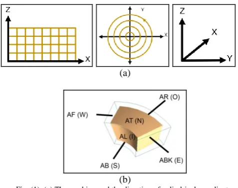
The bend mesh is generated using the straight pipe mesh with activating the parameter of the cylindrical coordinates.

The computational mesh was defined in a separate subroutine (MESHSET). A typical computational grid is illustrated in Figure (1) below:

(a)

(b)

Fig. (1). (a) The meshing and the direction of cylindrical coordinate; and (b) The six faces of a cell or a sub-mesh.

B. Simulation of Stratified Flow through Bend

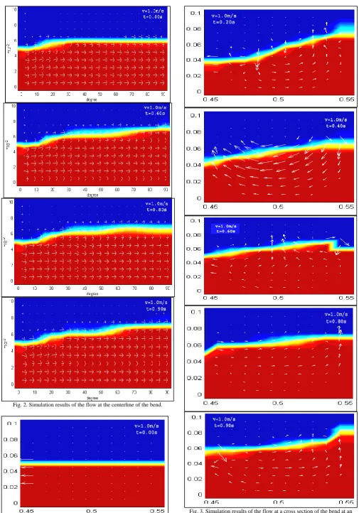
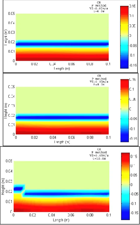
Fig. 2. Simulation results of the flow at the centerline of the bend.

Results depicted in Fig. 1 and (2) show the segregation of the phases. However, Fig. 2 shows a fluctuation in the value of the liquid film height at the inlet section and almost a stable higher value at the outlet section. This is consistent with the physical fact that the energy associated with the flow dissipates across the bend causing an accumulation of water at the outlet section.

Fig. 3 shows that the phenomenon of the piling effect at the right wall is significant during passing the bend. This phenomenon is associated with a clear disturbance caused by the secondary flow. Secondary flow, as shown, causes a change in the direction of the flow fields. At certain times (0.4 sec), the free surfaces tends to flatten once an equilibrium between the two opposite flow field directions could take place.

The vortex in the secondary flow is the main phenomena that causes pressure drop through bend. When liquid passes through a bend, the piling effect will happen near the outer radius. The right side of arrows show the liquid tends to pile up, however, the surface tension and gravitational force tend to pull down and flatten the liquid. The liquid flows to the left through the bottom of the pipe.

Several other simulation cases have been conducted with different parameters, locations and approaches. Acceptable agreements with experimental data were acquired.

C. Velocity Vector and Surface 3D Plot

Further efforts were carried out using Matlab to present a better visual of the 3D flow pattern. Sample of the 3D plot with velocity vector and surface functions is depicted in Fig. 4.

Fig. 4. Velocity vector and surface plot.

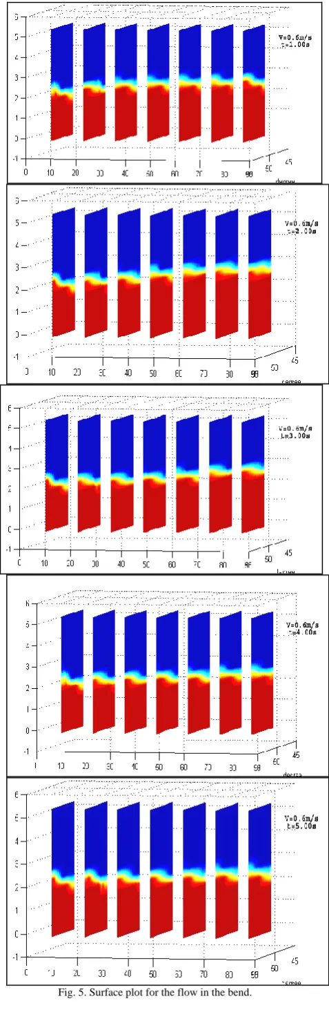
To avoid the complexity of Figure 4 above, an alternative approach has also been developed through surface plot with few planes arranged along the bend, as shown in Figure (5):

D. Wavy Flow Simulation

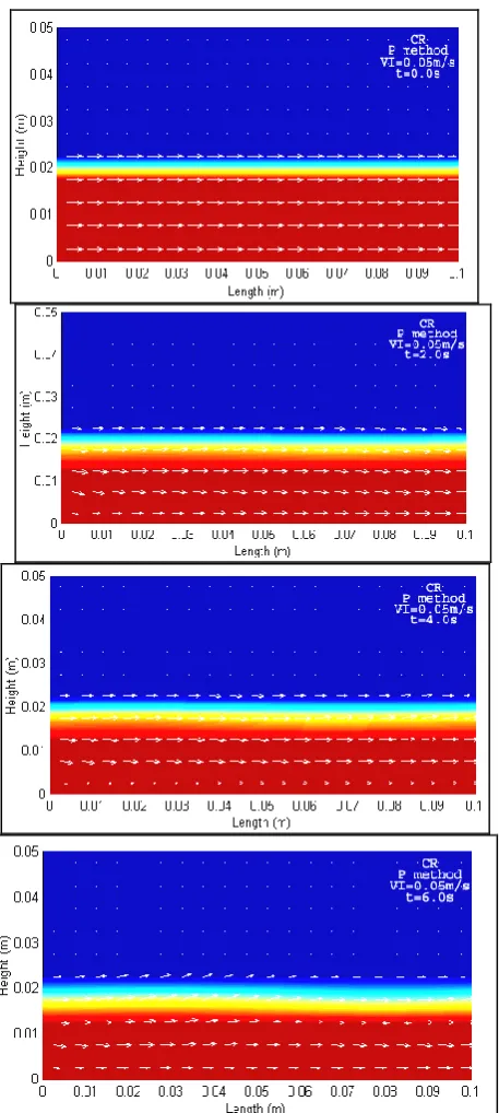
Simulation of stratified wavy flow is done through varying the surface pressure corresponding to the in-situ surface velocity. The interfacial shear stress is formulated into the surface cell pressure. For straight pipe, two alternatives were run to achieve an acceptable result on wavy flow pattern. First method is to add the interfacial shear stress into the subroutine of the boundary conditions while the second alternative is done on subroutine of the pressure in surface cells, obstacle cells and void cells.

The first modification done on the boundary condition method was to define the free-slip boundary for the circular section instead of no-slip wall, which is not suitable for large mesh. The second modification is to calculate the interfacial shear stress and to add into the surface cell pressure. Fig. 6 shows the stratified wavy flow for the modified boundary conditions in the mid-section of the pipe while Fig. 7 depicts the pressure distribution in that section.

Fig. 7. Pressure distribution of wavy flow with modified boundary conditions

The wave formation shown in Fig. 6 is due to interfacial shear stress. However, the gravitational force and surface tension tend to flatten the wave.

The results of pressure distribution presented in Fig. 7 show that the surface pressure is negative and lower than that at the no fluid cells. In other words, empty cells have zero pressure while the pressure of full fluid cells is differentiated by its hydrostatic value. The upper part is marked with lower hydrostatic pressure while the lowest fluid cells have the highest hydrostatic pressure. The surface pressure begins to change once the wave is generated.

The liquid film variations shown in these results reveals the fact that it's build up upstream of the bend part is the main reason for slug formation. The results of these simulations are consistent with the findings presented in [1], [3], [4].

REFERENCES

[1] A. Alwazzan, “Semi-empirical model to determine liquid velocity and pressure loss of two-phase flow in a horizontal bend – Part I (stratified flow),” International Journal of Petroleum Technology, vol .

2, no. 1, July 2015.

[2] A. Alwazzan, “Two-phase flow through horizontal pipe with bend,” PhD Thesis, University of Malaya, KL, Malaysia, 2006.

[3] A. Alwazzan and C. F. Than, “Calibration of a fiber optic sensing system for stratified flow in a pipe elbow,”National Conference on Engineering and Technology, Kuala Lumpur, Malaysia, May 26-27, 2004.

[4] A. Alwazzan, C. F. Than, M. Moghavvemi, and C. W. Yew, “Video imaging measurement of interfacial wave velocity in air-water flow through a horizontal elbow,”International Symposium of Photonics Systems and Applications, Singapore, November 26-30, 2001. [5] C. W. Hirt and B. D. Nichols, "Volume of fluid (VOF) method for the

dynamics of free boundaries," Journal of Computational Physics, vol. 39, pp. 201-225, 1981.

[6] K. Holmås, J. Nossen, D. Mortensen, R. Schulkes, and H. P. Langtangen, “Simulation of wavy stratified two-phase flow using computational fluid dynamics (CFD),” in Proc. 12th International Conference on Multiphase Production Technology, Barcelona, Spain 25-27 May, 2005.

[7] R. Khaksarfard, M. Paraschivoiu, Z. Zhu, N. Tajallipour, and P. Teevens, “CFD based analysis of multiphase flows in bends of large diameter Pipelines,”NACE Corrosion Conference, Orlando, Florida, 17-21 March, 2005.

[8] H. S. Kwak and K. Kuwahara, “A VOF-FCT method for simulating two-phase flows on immiscible fluids,” The Institute of Space and Astronautical Science, 1996.

[9] S. Lo and A. Tomasello, “Recent progress in CFD modelling of multiphase flow in horizontal and near-horizontal pipes,”in Proc. 7th North American Conference on Multiphase Technology, Banff, Canada, 2-4 June, 2010.

[10] Q. H. Mazumder, “CFD analysis of single and multiphase flow characteristics in bend,”Scientific Research – Engineering, pp. 210-214, 2012.

[11] B. D. Nichols, C. W. Hirt, and R. S. Hotchkiss, “SOLA-VOF: A solution logarithm for transient fluid flow with multiple free boundaries,” Technical Report LA-8355, Los Alamos National Laboratory, 1980.

[12] W. J. Rider and D. B. Kothe, “Reconstructing volume tracking,”

Journal of Computational Physics, vol. 141, pp. 112-152, 1998. [13] M. Rudman, “Volume-tracking methods for interfacial flow

calculations,”International Journal for Numerical Methods in Fluids, vol. 24, pp. 671-691, 1997.

[14] M. D. Torrey, L. D. Cloutman, R. C. Mjolsness, and C. W. Hewit, “NASA-VOF2D: A computer program for incompressible flows with free surfaces,”Technical Report LA-10612-MS, Los Alamos National Laboratory, 1985.

[15] M. D. Torrey, R. C. Mjolsness, and L. R. Stein, “NASA-VOF3D: A three dimensional computer program for incompressible flows with free surfaces,”Technical Report LA-11009-MS, Los Alamos National Laboratory, 1987.

[16] P. Vorobieff, C. A. Brebbia, and J. L. Munoz-Cobo, “Computational methods in multiphase flow VIII,”WIT Press, 2015.

[17] L.Xing and H. Yeung, “Investigation of slug flow induced forces on pipe bends applying STAR-OLGA coupling,” in Proc. 15th International Conference on Multiphase Production Technology, Cannes, France 15-17 June, 2011.