A Complete Study
of Algorithm Selection in Data
Mining
N.N.Krishnaveni
Assistant Professor, Holy Cross Home Science College, Tuticorin. India R.Waheetha
Assistant Professor, Holy Cross Home Science College, Tuticorin, India.
ABSTRACT:
Data mining involves the use of sophisticated data analysis tools to discover previously unknown, valid patterns and relationships in large data set. These tools can include statistical models, mathematical algorithm and machine learning methods. Consequently, data mining consists of more than collection and managing data, it also includes analysis and prediction. This paper puts forward the most used data mining algorithms used in the research field. With each algorithm, a basic explanation is given with a real time example, and each algorithms pros and cons are weighed individually. These algorithms are seen in some of the most important topics in data mining research and development such as classification, clustering, statistical learning, association analysis, and link mining.
Keywords: C4.5, K-means, SVM, Apriori, EM, Page Rank, k-nearest neighbor, Cart.
I. INTRODUCTION
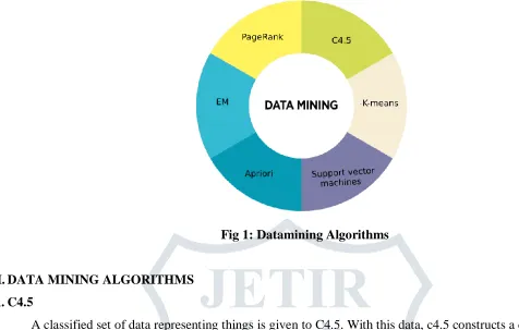
Fig 1: Datamining Algorithms
II.DATA MINING ALGORITHMS
A.C4.5
A classified set of data representing things is given to C4.5. With this data, c4.5 constructs a classifier in the form of a decision tree. Usually data mining uses classifier as a tool to classify a bunch of data representing things and predicts which class the data may be grouped to.
Example for C4.5:
To predict whether the patient will get diabetes or not. Hence performing C4.5 algorithm for the dataset which contains a bunch of patients details like age, blood pressure, and pulse rate, family history, VO2max etc. These are called as attributes. Now the patient’s data has to be grouped under two classes, Class 1 &Class 2: Whether the patient will get diabetes or not. From these attributes C4.5 can predict whether the patient will get diabetes. A decision tree is built from patients attributes and corresponding classes. This decision tree can further predict the class for new patients based on their attributes. The work of a decision tree is to create something similar to a flowchart to classify the data.
The algorithm, summarized as follows.
Algorithm 1:
Step 1:Create a node N;
Step 2:If samples are all of the same class, C then
Step 3: Return N as a leaf node labeled with the class C;
Step 4:If attribute-list is empty then
Step 5:Return N as a leaf node labeled with the most common class in samples;
Step6: Select test-attribute, the attribute among attribute-list with the highest information gain;
Step 7: Label node N with test-attribute;
Step 8:For each known value ai of test-attribute
Step 9:Grow a branch from node N for the condition test-attribute= ai;
Step 10:Let si be the set of samples for which test-attribute= ai;
Step 11:If si is empty then
Step 12:Attach a leaf labeled with the most common class in samples;
Step 13: Else attach the node returned by Generate_decision_tree(si,attribute-list_test-attribute)
Advantages:
The main reason to go for C4.5 would be its bestselling point of decision trees in their ease of analysis and explanation.
It also gives a fast response and is human readable.
Easily interpreted models can be built and implementation is easy.
Categorical values and continues values can be used and C4.5 deals with noise.
Limitations:
The limitations of this approach are that when the variable has close values or if there is a small variation in the data, different decision trees are formed.
Not suitable while working with small training set.
It is used in the decision tree classification for open source java implementation at open to x.
B.K-MEANS
intended to form groups such that group members are more similar versus non-group members. In clustering analysis, clusters and groups are synonyms.
Example for k-means:
For a dataset which consists of patient information: In cluster analysis, the data set is called as observations. The patient’s information includes age, pulse, blood pressure, cholesterol, etc. This is a vector representation of the data. Vector representation is in the form of a multi-dimensional plot. The list is interpreted as coordinates. Where cholesterol can be one dimension and age can be another dimension. From the set of vectors, K means does the clustering. The user only has to mention the number of clusters that are needed. K-means clustering operation has different types of variations to optimize for certain types of data. At a high level, k-means picks the different points and represents each of them k clusters. These are points are called as centroids. Every patient will be closest to any one of the centroids. They won’t be closest to the same one. Hence they will form a cluster around their nearest centroids. There are totally ‘k’ clusters. All the patients will be a part of a cluster.
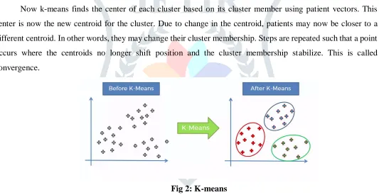
Now k-means finds the center of each cluster based on its cluster member using patient vectors. This center is now the new centroid for the cluster. Due to change in the centroid, patients may now be closer to a different centroid. In other words, they may change their cluster membership. Steps are repeated such that a point occurs where the centroids no longer shift position and the cluster membership stabilize. This is called convergence.
Fig 2: K-means
Figure 2 shows the data before K-means &after K-means. K-means algorithm can either be supervised or unsupervised. But mostly we would classify k-means as unsupervised. We call it unsupervised because k-means algorithm learns about the clusters on its own without any information about the cluster from the user. The user only has to mention the number the clusters that are required. The key point of using k means is its simplicity. It is faster and more efficient than other algorithms, especially for large datasets. k-means can be used in Apache Mahout, MATLAB, SAS R, SciPy, Weka, Julia,.
Advantages:
K-Means produce tighter clusters than hierarchical clustering, especially if the clusters are globular.
Limitations:
Difficult to predict K-Value, with global cluster.
Different initial partitions can result in different final clusters.
It does not work well with clusters (in the original data) of Different size and Different density.
C.SUPPORT VECTOR MACHINE (SVM)
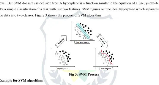
It classifies the data into two classes from the hyperplane. SVM performs a similar task like C4.5 at higher level. But SVM doesn’t use decision tree. A hyperplane is a function similar to the equation of a line, y=mx+b. It’s a simple classification of a task with just two features. SVM figures out the ideal hyperplane which separates the data into two classes. Figure 3 shows the process of SVM algorithm.
Fig 3: SVM Process
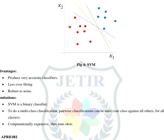
Example for SVM algorithm:
Fig 4: SVM
Advantages:
Produce very accurate classifiers.
Less over fitting
Robust to noise.
Limitations:
SVM is a binary classifier.
To do a multi-class classification, pairwise classifications can be used (one class against all others, for all classes).
Computationally expensive, thus runs slow.
D.APRIORI
It is applied to a dataset containing a large number of transactions. The algorithm learns associate rules. In data mining, associate rules are techniques for learning relations and correlations among variables in database.
Example for Apriori algorithm:
Consider the dataset of a supermarket transaction to be a giant spreadsheet. Each row of the spreadsheet is a customer transaction and every column represents a different grocery item. By using Apriori algorithm, we can analyze the items that are purchased together. We can also find the items that are frequently purchased than the other items. Together, these items are called item sets. The main aim of this is to make the shoppers buy more. Apriori is an unsupervised learning approach. It discovers or mines for interesting patters and relationships. Apriori can also be supervised to do classification on labeled data. Apriori can be used for ARtool, Weka, and Orange.
Working of Apriori:
The size of the item set (If you want to see the patterns for 2-itemset, 3-itemset, etc.?).
The number of transactions containing the item set divided by the total number of transactions.
A frequent item set is one which meets the support and Confidence or conditional probability. Advantages:
It uses large item set property.
Easily Parallelized.
Easy to implement. Limitations:
Assumes Transaction database is memory resident.
Requires many database scans.
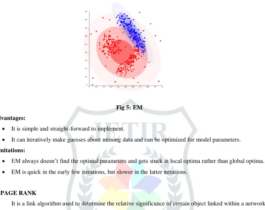
E. EXPECTATION-MAXIMIZATION (EM)
It is a commonly used as clustering algorithm for knowledge discovery in data mining. It is similar to k-means. While figuring out the parameters of a statistical model with unobserved variables, the EM algorithm optimizes the likelihood of seeing the observed data. Statistical model is describing how observed data is generated. The EM algorithm is unsupervised as it is not provided with labeled class information.
Example for EM:
The grades for an exam are normally distributed using a bell curve. Assume that this is the model. Distribution is generally the probabilities for all measurable outcomes. The normal distribution of the grades for an exam represents all the probabilities of a grade. Or it is the determination of how many exam takers are expected to get that grade. A normal distribution curve has two parameters: The mean and the variance. In certain cases, the mean and the variance may not be known. But still we can calculate the normal distribution using the sample case. For example, we have a set of grades and are told the grades follow a bell curve. However, we’re not given the grades but only a sample. Using these parameters, the hypothetical probability of the outcomes is called likelihood.
Keeping in mind that it’s the hypothetical probability of the existing grades and not the probability of a future grade. Probability is estimating the possible outcomes that should be observed. Observed data is the data that you recorded. Unobserved data is data that is missing. There are many reasons that the data could be missing (not recorded, ignored, etc.). By optimizing the likelihood, EM generates a beautiful model that assigns class labels to the different data points. EM algorithm helps in the clustering of data. It begins by taking a guess at the model parameters. Then it follows a three step process:
E-step: The probabilities for assignment of each data point to a cluster are calculated. This is done based on the model parameters.
Fig 5: EM
Advantages:
It is simple and straight-forward to implement.
It can iteratively make guesses about missing data and can be optimized for model parameters.
Limitations:
EM always doesn’t find the optimal parameters and gets stuck in local optima rather than global optima.
EM is quick in the early few iterations, but slower in the latter iterations.
F. PAGE RANK
It is a link algorithm used to determine the relative significance of certain object linked within a network of objects. Link analysis is similar to network analysis which is looking to search the association among links. The most common example for page rank is Google’s search engine. Though, the search engine doesn’t solely rely on page rank. It’s one of the measures goggle uses to determine a web page importance.
Advantages:
Robust against spam.
Global measure.
Query independent.
Limitations:
Favors older pages
G.K-NEAREST NEIGHBORS (KNN)
It stands for k-Nearest Neighbors. It is a classification algorithm which differs from the other classifiers previously described because it’s a slow learner. A slow learner only stores the training data during training process. It classifies only when a new unlabeled data is given as input. On the other hand, a fast learner builds a classification model during training. When new unlabeled data is given as input, this type of learner feeds the data into the classification model. C4.5 and SVM are both fast learners because: SVM builds a hyperplane classification model during training. C4.5 builds a decision tree classification model during training. kNN builds no such classification model as seen above. Instead, it just stores the initial labeled training data. When new unlabeled data comes in, kNN operates in 2 basic steps:
First, it looks at the closest labeled training data points.
Second, using the neighbors’ classes, kNN gets a better idea of how the new data should be classified. For figuring out the closest data, kNN uses a distance metric like Euclidean distance. The choice of metric for the distance largely depends on the data. Some even suggest learning a distance metric based on the training data. There’s a lot of detail and many papers on kNN distance metrics. For data that is discrete, the idea is to transform the obtained discrete data into continuous data. 2 examples of this are: Using Hamming distance as a metric for the “closeness” of two text strings and hence transforming discrete data into binary features. kNN has an easy time when all the neighbors are of the same class. The basic feeling is if all the neighbors agree, then the new data point is likely to fall in the same class. Two common techniques for deciding the class when the neighbors don’t have the same class is to take a simple majority vote from the neighbors. Whichever class has the greatest number of votes becomes the class for the new data point. Take a similar vote, except this time give a heavier weight to those neighbors that are closer. A simple way to implement this is to use reciprocal distance.
For example, if the neighbor is 5 units away, then the weight of its vote is 1/5. As the neighbor gets further away, the reciprocal distance gets smaller and smaller. kNN is a supervised learning algorithm as it is provided with labeled training dataset. A number of kNN implementations exist in MATLAB knearest neighbor classification, scikit-learn KNeighborsClassifier and k-Nearest Neighbor Classification in R.
Advantages:
Depending on the distance metric, kNN can be quite accurate.
Disadvantages:
Noisy data can throw off kNN classifications.
kNN can be computationally expensive when trying to determine the nearest neighbors on a large dataset.
kNN generally requires greater storage requirements than faster classifiers.
Selecting a good distance metric is crucial to kNN’s accuracy.
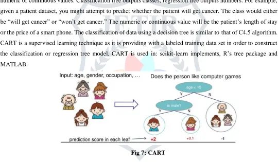
H.CART:
CART stands for Classification and Regression Trees. It is a decision tree learning technique similar to C4.5 algorithm. The output is either a classification or a regression tree. In simple, CART is a classifier. A classification tree is a type of decision tree. The output of a classification tree is a class. A regression tree predicts numeric or continuous values. Classification tree outputs classes, regression tree outputs numbers. For example, given a patient dataset, you might attempt to predict whether the patient will get cancer. The class would either be “will get cancer” or “won’t get cancer.” The numeric or continuous value will be the patient’s length of stay or the price of a smart phone. The classification of data using a decision tree is similar to that of C4.5 algorithm. CART is a supervised learning technique as it is providing with a labeled training data set in order to construct the classification or regression tree model. CART is used in: scikit-learn implements, R’s tree package and MATLAB.
Fig 7: CART
Advantages:
Builds models that can be easily interpreted.
Easy to implement.
Can use both categorical and continuous values.
Deals with noise.
III. CONCLUSION
database management system. We have observed a large number of algorithms to perform data analysis tasks. We hope this paper inspires more research in data mining so as to further explore these algorithms, including their many impact and look for new research issues.
REFERENCES
[1] Baik, S. Bala, J. (2004), A Decision Tree Algorithm for Distributed Data Mining: Towards Network Intrusion Detection, Lecture Notes in Computer Science, Volume 3046, Pages 206 – 212.
[2]Bouckaert, R. (2004), Naive Bayes Classifiers That Perform Well with Continuous Variables, Lecture Notes in Computer Science, Volume 3339, Pages 1089 – 1094.
[3] Breslow, L. A. & Aha, D. W. (1997). Simplifying decision trees: A survey. Knowledge Engineering Review 12: 1–40.
[4] Brighton, H. & Mellish, C. (2002), Advances in Instance Selection for Instance-Based Learning Algorithms. Data Mining and Knowledge Discovery 6: 153–172.
[5] Cheng, J. & Greiner, R. (2001). Learning Bayesian Belief Network Classifiers: Algorithms and System, In Stroulia, E. &Matwin, S. (ed.), AI 2001, 141-151, LNAI 2056,
[6] Cheng, J., Greiner, R., Kelly, J., Bell, D., & Liu, W. (2002). Learning Bayesian networks from data: An information-theory based approach. Artificial Intelligence 137: 43–90.
[7] Clark, P., Niblett, T. (1989), The CN2 Induction Algorithm. Machine Learning, 3(4):261-283.
[8] Cover, T., Hart, P. (1967), Nearest neighbor pattern classification. IEEE Transactions on Information Theory, 13(1): 21–7.
[9] D. Michie, D.J. Spiegelhalter, C.C. Taylor “Machine Learning, Neural and Statistical Classification”, February 17, (1994).
[10]DelveenLuqman Abd Al.Nabi, Shereen Shukri Ahmed, “Survey on Classification Algorithms for Data Mining: (Comparison and Evaluation)” (ISSN 2222-2863)4(8); (2013)