Fit Generalized Linear Models by Using of Different Likelihoods

Fit Generalized Linear Models by Using of Different

Likelihoods

Hoda Rashidi Nejad

1 1_{Graduated student, Kerman, Iran}

Abstract-- Regression models have wide applications in analysis of data with continues and normal distributed responses. Extended of these models happens when these distribution of responses are not normal but they belong to the distribution of exponential family. It is called generalized linear model(GLM). S tatistical inference of glm usually is done based on full likelihood, however computing of full likelihood is hard in some complex models, that needs using of replacement other likelihoods such as: profile likelihood, conditional or marginal likelihoods, empirical likelihood and quasi likelihood. There for using these likelihoods is more applicable than full likelihood. In this research, various likelihood functions for prediction of variables in models are proposed. The main objective of this research project is to overcome the difficulties of using the full likelihood and its related calculations which has been done by application of other likelihoods. Also we work on tentative data of productivity of bulldozer and fit models and compare the error of three models.

Index Term-- Link function, nuisance parameter, quasi likelihood, sufficient statistics.

I. INT RODUCT ION

Models have been used for many years for the analysis of non -normal data. The probit regression model used for a binary response is a classic example. The concept of probit was previously used by [1] and [2]. The principle of probit regression was used by [3] for solving psychology problems. [4] introduced maximum likelihood estimators for finding solutions to problems.

Generalized linear models can deal with probit or logistic regression, Poisson regression, logarithmic linear models for cross tables, estimates of the variance component of the mean squares of ANOVA, etc. Most of the problems that we deal with are multiparameter models; for example, the normal

model

N

( ,

 

2

)

has two parameters that must be computed. The complexity of the model is determined by the number of parameters in it. The likelihood function is in the form of

( )

( )

L





P y

_ , where

P y

_

( )

is the probability of the observed data. When the likelihood function has more than one parameter, use of the full likelihood is difficult. When the inference of several parameters is important, it is preferable at any time to carry out the inference on one of the parameters, and then carry out the same for the remaining parameters. In some models, there may be several parameters, but only one of them is important. For example, in a normal model,



is an important parameter, whereas



2 is a nuisance parameter. In this case, the preferred method is to compute the maximum likelihood estimator (MLE) of the nuisance parameter using the likelihood function by assuming a fixed value for the important parameter and then replacing the nuisance

parameter in the model with this value, thus deleting the nuisance parameter. This type of likelihood is called profile likelihood. In cases where the computation of the MLE of the nuisance parameter is difficult, we can express a conditional likelihood for simplicity. The advantage of co nditional likelihood over profile likelihood is that in concept, they are similar to the probability of the observed data. Though gain to a model without nuisance parameter is not clear but we t ry to make the inference of models easy, with the likelihoods that we introduce in this paper.

In this paper, we first introduce generalized linear models and their properties in section 2. In section 3, the profile likelihood is introduced and in section 4, the conditional and marginal likelihoods are discussed. In section 5, the empirical likelihood is introduced. Then, in section 6, the quasi likelihood is presented and finally, we present a real example in which we use some of these likelihoods for fitting a model and compute their errors.

II. GENERALIZED LINEAR MODELS(GLM)PROCEDURE FOR

PAPER SUBMISSION

In general, a GLM consists of three components:

a) The random component: The dependent variable (y), containing the observations

y

_i, which are assumed to be independent and have a distribution of the exponential family.

b) The systematic component: It includes the linear predictor





X



, where



is a

P



1

vector of unknown parameters and

X

is an

n P



matrix of independent variables.

c) The link function: This is a univocal ascendant function and can be derived once, the relation between the systematic component of the model and the expectation of the random variable (

E Y

( )





) is determined. The link function is denoted by g in the equation





g

( )



.

It is usually supposed that the vector

Y

contains independent indicators of a distribution with density function of the exponential family as below

~

.

( )

[

( )]

( )

exp

( , ) .

( )

i

i

i Y i

i i i

Y i i

y

indep f

y

y

b

f

y

c y

a





_











_



_





(1)

unique properties. Table I shows some canonical link functions with well-known distributions.

Usually, the relations between the distribution parameters and the different predicted variables are of interest, that computed

with modeling of one reduction of the mean of



_i which is a

function of



_i, of a linear model in predictors.

( )

_i





_i

,

(



_i

)



_i





.

E Y

g

X

(2)

where g(.) is a known function called the link function

(because it links the mean of the

y

_is and the linear predictors),

X

_i



and



are the ith row of the model matrix and parameter vector for the linear predictors, respectively. We have to decide which predictors are at the right hand side of (2) and what form they take. The goal in a GLM is that obtain estimates of the parameter



. The log likelihood for (1) is

1 1

[

( )]

( , )

( )

n n

i i i

i

i i

y

b

l

C y

a





_



 











We can write the log likelihood function as a derivative of



:

1

(

)

(

)

( )













_









i i i i i

l

y

w g

X

a

where

w

_i





v

(



_i

)

g

_2

(



_i

)



1.

This can be written in the matrix form as follows:

1

(

)

( )

l

a







_







X WΔ Y μ

where

W



{ }

w

i and

Δ



{

g



( )}



i . The maximu m likelihood equation is













W

y

X

W

X

(3)

Where

W

,



, and



include the unknown parameter



. Usually, these terms are nonlinear functions of



and therefore (3) cannot be solved algebraically. To solve the maximum likelihood equations or compute the variance, it is useful to have the expectation of the second derivative of the log likelihood. We notice that

2

1

( )

1

(

)

( )

l

X W

a

W

X

y

a



 













_{ }

_

_







 



 











Then we will have

2

1

( )

l

E

X WX

a

 









_



_

_





 





To find the variance of



ˆ

we first notice that

2 2

1

[

]

( )

( )

0.

l

E

X W E y

a

a















_



_

_







 







(4)

Therefore, the estimation of

a

(



)

has no effect on the variance of



ˆ

. It can easily be shown that

1

ˆ

( )

( )(

)

Var





a



X WX





By regarding that the information matrix

I

( )



is

( )

l

l

I



E

 



 



 

_{ }

_







,

the variance-covariance matrix of



ˆ

will be





1

ˆ

( )

( )

Var





I



 .

Solving the maximum likelihood equations (3) for



is normally done by the reweighted least squares method. This method is similar to the Fisher scoring algorithm [5].

Fisher scoring is a repetitive method used for likelihood maximization, which can be represented by the followin g form: ) ( 1 ) ( ) ( ) 1 (

)

(

m

l

I

m m m  









  _









(5)

where m represents the mth repeat,

I

(



)

is the information matrix, and



is the full parameter vector. By using (5) and (4) for



, we have

)

(

)

(

1 ) ( ) 1 (























y

W

X

WX

X

m m

where

W

,



and ,



are computed for



(m). III. PROFILE LIKELIHOOD FUNCT ION

Given

L

( , )

 

such that

( , )

 

are function parameters and



is the parameter of interest, the profile likelihood for



is

( )

max ( ; )

L

L







 

The maximum is reached when

L

( )

max ( ; )

L







 

is

fixed. That means , for a fixed



, the MLE for



generally is a function of



[6]. Therefore, we can write,

TABLE I

SOME CANONICAL LINK FUNCTIONS

Distributions Canonical link function

Normal i i

 



Binomial

log

1

i i i

p

p







Poisson

log(

)

i i







Exponential

1

i i







Gamma (fixed



)

ˆ

( )

( ,

)

L





L

 

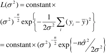
_ . Hence, the profile likelihood is a regular likelihood. For example, we can base the inference on the likelihood function.

Example 1. Suppose that

y

₁

,

,

y

n is an identically independently distributed (i.i.d) sample of

N

( ,

 

2

)

with unknown parameters. The likelihood function of

( ,

 

2

)

is

2 2

2 2

1

1

( ,

)

exp

(

)

2

2

n

i i

L

 

y

















_

_

_





_











For a fixed



, the MLE for



2 is

2

1

2

(

_i

)

i

y

n













Therefore, the profile likelihood of



is

2 ₂

ˆ

( )

constant (

) .

n

L









_ 

This profile likelihood differs from the estimated likelihood expressed below:

2 2

2

2

ˆ

( ,

)

constant

1

exp

(

)

.

ˆ

2

i i

L

y

 















_

_













If



2 is well estimated, then these two likelihoods will be close in value; otherwise, the profile likelihood is preferred.

Fig. 1. Profile likelihood for mean



(continuous line),

2

_ˆ

2

( ,

)

L

 





(broken line), and

L

( ,

 

2



1)

(dotted line)

( )

L



and

L

( ,

 

2





ˆ

2

)

for the observed data are shown in Figure 1. It is clear that for an unknown parameter and

assuming



2



1

, we reach the wrong inference. Therefore, in general, a nuisance parameter to improve the model is needed, although it must be deleted by an appropriate method.

We also compute the profile likelihood for



2 as follows:





2

2 ₂ 2

2

2

2 ₂

2

(

)

constant

1

(

)

exp

(

)

2

ˆ

constant (

)

exp

.

2

n

i i n

L

y

y

n











_











_

_



















IV. MARGINAL AND CONDIT IONAL LIKELIHOOD

In statistics, a marginal or integrated likelihood function is a function in which some of the variables of its parameters have become ancillary. Assuming that





( , )

 

, where



is a parameter of interest, it is often desirable to introduce the likelihood function into



. If there is a probability function for



(in some cases, it is called the nuisance parameter) conditioned on



, then we may take an integral over



. This means

( ; )

( | )

( | , ) ( | )

L



x



p x







p x

 

p

  

d

We now obtain the marginal likelihood for computing the conditional likelihood. In some cases we may find a sufficient statistic for the nuisance parameter, and with a conditioned likelihood on this, we can reach the conditional likelihood[6].

Assume that the log likelihood for





( , )

 

is

( , )

t

( )

l



y





s b





and that

l

( , )



y

can be expressed as

1 2

( , )

t t

( , )

l



y





s





s



b

 

which is valid when



is a linear function of



. The choice of the nuisance parameter (



) is arbitrary and the inference of



is not influenced by the choice of



. The conditional likelihood of

Y

conditioned on

s

₂, is

*

2 1 2

( |

)

t

( , )

l



s





s



b



s

which is independent of the nuisance parameter and may be used for inference of the parameter



. For a general method, assume a reduction of

x

data like

( , )

v w

so that the marginal distribution of

v

or conditional distribution of

v

conditioned on

w

, dependents only on the parameter of interest



. Assume that the full parameter is

( , )

 

. In the first situation, we have

,

,

1 2

( , )

( , )

( )

(

)

( )

( , )

L

P

v w

P v P

w v

L

L

 

  

 



 







Therefore, the conditional likelihood of



is defined as

1

( )

( )

L





P v

_

In the second situation, we have

,

1 2

( , )

(

)

( )

( )

( , )

L

P v w P

w

L

L

  

 



 





1

( )

(

).

L





P v w

_

Choosing any of these two above likelihoods depends on the interested problems. However, if v and w are independent, the two likelihoods are the same.

V. EMPIRICAL LIKELIHOOD

Empirical likelihood is defined as

1

( )

sup

( )

n

F i

i

L

P













That supremum is taken on all of the possible functions

F

_ on

1

,

,

n

x

x

, such as

t F

(

_

)





. The distribution

F

_ is specified by the probabilities



P

_i

( )





on

x

₁

,

,

x

_n.

The function

t F

( )

describes a specific item of distribution. For example, the mean of F is the function

( )

( )

t F





xdF x

. Other examples are the variance,

skewness, etc.

VI. GENERAL QUASI LIKELIHOOD

We obtain the uses of known functions

f

(.)

and

g

(.)

for a definite outcome

y

_i and predictor

x

_i so that

(

_i

)

_i

g





x





, or

E Y

( )

_i





_i



f x

(

_i





)

such that

g

(



_i

)

is a link function and we have

( )

_i

(

_i

)

Var y



 

v

. Assume a model where the ith proportion of the log likelihood is



( )



log

i i i i

(

i

, )

y

A

L





c y











(6)

with a known function

A

(.)

. The function

c y

(

_i

, )



is necessary for the definition of

A

(.)

because the integral over this density must be equal to 1. In estimates of standard quasi likelihood, it is not necessary to know the value of

c y

(

_i

, )



because there are implicit formulas for several models, otherwise we can use the generalized quasi likelihood function below. The score function and Fisher information are obtain ed as follows:





2

2

( )

log

( )

log

.

i i

i i

i

i

i i

i

y

A

S

L

A

I

L





























 





If

A

( )



_i is chosen such that

( )

_i

( )

_{i i}

E Y



A









and

( )

i

( )

i i

(

i

)

Var Y





A







 

V

,

then the likelihood is the established discipline qualification

(

i

)

( )

i

Var S



E I

and

E S

(

i

)



0

The regression model with the link function

g

(.)

is

(

_i

)

_i

g





x





where

g

(.)

is the linear prediction criterion. It can be shown that the score function

S

( )





0

is equal to the estimate

equation 1

1

(

)

0

n i

i i i

i

V

y



_









_

_





. This means that the

likelihood of the exponential family (6) is stable for a wide class of distributions that are specified by consistent likelihood since the mean and variance of the model are specified correctly [6].

VII. EXT ENT ION

Consider a quasi likelihood model. The proportion of the

log likelihood of a single observation

y

_i is

{

( )}

log ( , )

i i i

(

, )

i i

y

A

L

 





c y











when the function

c y

(

i

, )



is unknown. a straight estimate

of



is not possible. An approximation is obtained as follows

1

log ( , )

log(2

( ))

2

1

( ,

)

2

i i

i i

L

V y

D y

 







 



using the deviance

(

,

1;

)

(

,

)

2 log

(

,

1;

)

i i

i i

i i

L y

y

D y

L

y





 







where

L

(

 

i

,



1;

y

i

)

is the likelihood of



i based on a single observation of

y

_i with the assumption of





1

. This type of likelihood is termed as an extension likelihood [7].

VIII. ACASE EXAMPLE

Consider the study data of [8] about the productivity of a bulldozer. We want to fit the following model with the data

under the assumption that



_i

~

N

(0,



_e2

)

:

0 1 3 2 4

3 9 4 12 5 15

6 16 7 17

,

1,

, 60

i

i

y

X

X

X

X

X

X

X

i







































This model was fitted in the study conducted by [8]. We now want to fit this model using the conditional and profile likelihoods explained in the previous sections, with a deleted

nuisance parameter (



_e2) and then compare the three models. In the conditional model, the likelihood is conditioned on

sufficient statistic of



_e2 that is equal to

(

_i

)

2

i

y



X







. In

Fig. 2. shows the errors in the models computed by these two likelihoods and the errors in the previous regression model.

As shown in Fig. 2, the errors of models fitted by conditional likelihood are the lowest. And the regression errors are lower than models fitted using profile likelihood. Therefore, for these data, the model fitted by the conditional likelihood is the best model.

REFERENCES

[1] David, H.A. Fist Occurrence of com m on term s in m athem atical statistics. T he American statistician, 29:21-31. 1995.

[2] Bliss, C. The m ethod of probits. Science, 79:38-39. 1934.

[3] Finney, D.J. Probit analysis. Cambridge university press, Cambridge. 1952.

[4] Fisher, R.A. Appendix to the calculation of the dose-mortality curve(by Bliss). Annals of applied biology, 22:164-165. 1935

[5] S.R. Searle, G. Cassella and C.E. McCulloch. Variance com ponents. Wiley, New York. 1992.

[6] Pawitan, Y. In all likelihood: Statistical modeling and inference using likelihood. Clarendon Press-Oxford. 2001.

[7] Nelder, J.A. and Prigibon, D. An Extended quasi-likelihood function. Biometrika, 74: 221-132.

[8] A. Rashidi, H. Rashidi Nejad and A.H. Behzadan. Multiple linear regression approach for productivity of bulldozers. Korean conference of Construction Engineering and Management(ICCEM, ICCPM). 2009.

TABLE II

COMP UTED PARAMETERS OF TWO LIKELIHOODS

Parameters

7





₆

5



4





₃

2



1





₀

-4.17 -1.1 -2.21 -7.71 12.6 10.62 -6.97 82.16 Regression

-27.04 -1.33 -3.33 5.11 20.9 10.61 -3.62 -79.34 Conditional likelihood