Modeling flexibility using artificial neural networks

R E S E A R C H

Open Access

Modeling flexibility using artificial neural

networks

Kevin Förderer

, Mischa Ahrens

, Kaibin Bao

, Ingo Mauser

and Hartmut Schmeck

FromThe 7th DACH+ Conference on Energy Informatics Oldenburg, Germany. 11-12 October 2018

*Correspondence:[email protected] 1_{FZI Research Center for} Information Technology, Haid-und-Neu-Str. 10-14, 76131 Karlsruhe, Germany

Full list of author information is available at the end of the article

Abstract

The flexibility of distributed energy resources (DERs) can be modeled in various ways. Each model that can be used for creating feasible load profiles of a DER represents a potential model for the flexibility of that particular DER. Based on previous work, this paper presents generalized patterns for exploiting such models. Subsequently, the idea of using artificial neural networks in such patterns is evaluated. We studied different types and topologies of ANNs for the presented realization patterns and multiple device configurations, achieving a remarkably precise representation of the given devices in most of the cases. Overall, there was no single best ANN topology. Instead, a suitable individual topology had to be found for every pattern and device configuration. In addition to the best performing ANNs for each pattern and configuration that is presented in this paper all data from our experiments is published online. The paper is concluded with an evaluation of a classification based pattern using data of a real combined heat and power plant in a smart building.

Keywords: Smart Grid, Modeling, Flexibility, Distributed energy resources, Demand side management, Machine learning

Introduction

Traditionally, electricity has almost exclusively been produced in large power plants connected to electricity transmission grids. The growing share of distributed energy resources (DERs) connected to distribution grids makes reliable grid operation increas-ingly challenging. Since solar and wind energy are volatile in nature, generation by DERs that use these energy sources is intermittent. To limit the extent of necessary grid and energy storage expansion, the exploitation of the already existing flexibility of DERs like battery energy storage systems (BESSs) and combined heat and power (CHP) plants is essential. Aside from conventional measures of demand response (DR), newer approaches to achieve a comprehensive demand side management (DSM) (Palensky and Dietrich

2011) have been proposed, including hierarchical (Molderink2011; Anders et al.2014; Toersche et al.2015), distributed (Callaway and Hiskens2011; Hinrichs and Sonnenschein

2017), decentralized (Bremer and Lehnhoff 2017; Rohbogner et al. 2014) and cellular systems (Mauser et al. 2017b; Waffenschmidt2017). A common necessity for all these approaches is the need to at least model and often communicate flexibility.

The flexibility of a particular DER or an aggregate of multiple DERs can be described as the set of allfeasibleload profiles for a given time frame. Feasible in the context of DER load profiles refers to load profiles that can be realized based on the current state while providing all necessary services (Mauser et al.2017a). In this paper we pick up the idea of representing and communicating flexibility withartificial neural networks(ANNs) pre-sented in (Förderer et al.2018): A single ANN implicitly learns a flexibility model for one or multiple aggregated DERs using generated or measured load profiles and state data relating to the corresponding DERs as training data. It is important to note that a single (measured) load profile does generally give only few clues about the available flexibility. In order to derive an adequate description of the flexibility in a given state, a sufficient num-ber of measured load profiles with comparable initial states is required. Since the ANNs can be trained to consider these initial states, they should be able to deduce the actual flexibility. The ANNs are trained locally and then transmitted to third parties to offer flexibility information and act assurrogate models. Depending on the chosen training pat-tern, such an ANN could, e.g., evaluate if a given load profile is feasible for a particular DER. This approach enables the abstraction and communication of distributed flexibility regardless of the type, configurations and sizes of the considered DERs. Since a trained ANN may factor in the current state of the corresponding DERs, it is sufficient to only communicate states rather than a complete model once an ANN is known.

This paper aspires to evaluate the idea of using ANNs as surrogate models for flexibility by testing the effectiveness of different ANN types and topologies in conjunction with thepatternspresented in (Förderer et al.2018). By explaining the particularly good or bad results achieved for a given pattern and DER configuration, we aid future research in designing better ANNs that represent energy flexibility. An additional evaluation is conducted using real-world CHP data for one of these patterns.

Related work

As mentioned before, this paper is based on the ideas outlined in (Förderer et al.2018). Due to the variety of possible applications for the concept and patterns, the presented results are related to a multitude of previous publications. In this section we give a brief overview of findings motivating the concept and point out important distinctions from other related work.

Regardless of using direct or indirect mechanisms for controlling DERs (Mauser et al.

2017a), it is necessary to employ some sort of model to determine flexibility. For exam-ple, customers may respond diversely to time-of-use tariffs (Faruqui and George2005; Faruqui and Sergici 2010) and even these responses are heavily influenced by local parameters (Jargstorf et al.2015). Hence detailed models and information are needed.

In contrast to these, in the concept presented in (Förderer et al.2018) and evaluated in this paper the ANN is generated locally but used externally by a third party.

Regarding the concept and the patterns evaluated in this paper,support vector data description (SVDD) (Bremer et al. 2011; Bremer and Sonnenschein 2013; Nieße et al.

2016; Bremer and Lehnhoff2017) and thecascade classification model (Neugebauer et al.2015; Neugebauer et al.2016; Neugebauer et al.2017) are the most relevant related approaches. SVDD can be used to decide whether a load profile is feasible for a particular DER or an aggregate of DERs or not. Additionally, SVDD (in theory) allows for repair-ing infeasible load profiles. An important distinction to the models used in this paper is that the SVDD model must be generated each time the flexibility is exchanged. The cas-cade classification approach is an example for an application of the classification pattern discussed in the next section.

Approach

Someone who seeks to generate suitable signals, i.e. incentives or commands, in order to influence generation and consumption generally bases their decisions on descriptions of the available flexibility. These descriptions are given by one or multiple models for the flexibility provided by DERs. Since flexibility can be seen as a set of feasible load profiles, the basic function of a model for flexibility is to enable an operator to find suitable profiles. The set of feasible load profiles is often modeled by specifying the definitive constraints. However, any other model allowing the generation of feasible load profiles, e.g. a simple enumeration of load profiles, can pose as a model for the flexibility of DERs.

Realization patterns for modeling flexibility

The patterns outlined in this section are a generalization of the five usage patterns for ANN-encoded abstracted flexibility presented in (Förderer et al.2018). We omit pattern Ewhich allows the optimization and communication of load changes rather than absolute load profiles, since it is basically an extension of the other patterns. Each pattern corre-sponds to pattern specific (surrogate) models. Given one of these pattern specific models, the pattern can be used to generate a set of feasible load profiles. Thereby, the pattern specific model acts as a model for the flexibility of DERs. In the following, we refer to all kinds of third parties performing DSM, e.g. electric utilities (Gellings1985) or dedicated regional EMSs (Kochanneck et al.2015), with the termdemand side manager(DSMgr). For simplicity, we use the termbuildingwhen referring to a provider of flexibility. Never-theless, the concept is applicable to any kind of energy system, such as a single household, a multi-family building, a commercial or industrial property, or avirtual power plant

aggregating multiple DERs. Since there are many more possibilities to achieve the goal of generating feasible load profiles, the list of patterns is not exhaustive.

Pattern A: load profile classification

Pattern B: price-based load profile forecasting

Theprice-based forecasting patternemploys a model that forecasts a load profile for a given arbitrary price signal. By applying the model to various price signals, again, a set of load profiles is generated. After determining the optimal profiles, the corresponding price signal is sent to each building.

Pattern C: load profile generation

In the generation pattern, the models are used to generate valid load profiles from arbitrary representations. An intuitive type of representation is, for example, a control sequence specifying how a DER operates. By processing the commands in the control sequence the model can generate a load profile. Another type of (latent) representation, usually used in Generative Adversarial Networks, is a vec-tor of random variables. Given a model, the DSMgr creates representations either randomly or according to an algorithm and generates a feasible load profile from each representation. In this pattern, like in pattern A, load profiles are selected and transmitted.

Pattern D: load profile validation and repair

Thevalidation and repair patternis based on models that allow transforming infeasible load profiles into feasible profiles. Already feasible profiles either remain unchanged when the model is applied or are filtered beforehand, e.g. through patternA. In addition to allowing the generation of feasible load profiles, thevalidation and repair patterncan simplify the directed search for feasible load profiles if the transformed, i.e. repaired, load profile is similar to the profile given to the model. Again, the target is the identification and communication of desired load profiles.

Communication

In order to utilize the models for flexibility they need to be available to the DSMgr. Based on the previous section and again (Förderer et al.2018), this section discusses the transmission and general utilization of the models. For this purpose, quantities are dis-tinguished betweenparametersandvariables. More precisely, parameters are constants inherent to an energy system and variables reflect the current state of the system. A BESS, for instance, can be modeled with the parameter ‘storage capacity’ that remains fixed and the variable ‘state of charge’. Regarding the communication, the model and its parameters only need to be transmitted once. Variables, on the other hand, reflect the current state of the system and thus have to be updated repeatedly.

In detail, initially and whenever the model and/or parameters are outdated, new models are generated and parameters are determined by the EMS of the building and transmitted to the DSMgr’s EMS (see Fig.1):

1. Generate a model and determine the parameters in the local EMS of the building according to the particular usage pattern (cf. patternsAtoD)

2. Transmit the model and parameters to the DSMgr

3. Store the received information in the EMS of the DSMgr for later usage

Building

Demand Side Manager

Energy Management

System

Energy Management

System Flexibility

Model & Parameters

(1) Train

(2) Transmit

(3) Store

Fig. 1Model and parameters representing the flexibility of one or multiple DERs in a building are communicated to the demand side manager (cf. (Förderer et al.2018))

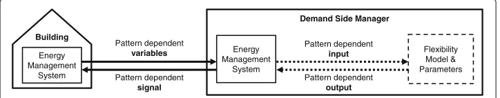
Figure2depicts the process of generating feasible load profiles in order to determine a signal for influencing the behavior of the building. Periodically or on demand, the EMS of the building sends the variables relevant to the applied pattern to the DSMgr’s EMS. The EMS of the DSMgr then uses the model and parameters it has previously stored, the pattern dependent variables and additional pattern specific inputs (cf. patternsAtoD) to find the optimal load profile and thereby determine the signal to be sent to the EMS of the building.

Concept of ANN-encoded flexibility

In this paper we evaluate the concept ofANN-encoded abstracted flexibilitypresented in (Förderer et al.2018). Therefore, the models for applying the patterns are all based on ANNs. The ANNs represent one or multiple DERs and act assurrogate models. We assume that the variables provided by the building contain the current state of the DERs that are represented by the ANN. The ANN input is then the current state and some pattern specific data (see above) that needs to be generated by the EMS of the DSMgr. Table1provides a summary of the pattern specific input and output of the ANNs.

Methodology and models

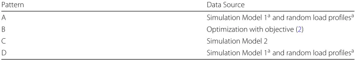
Although the patterns presented in this paper all serve the same purpose, which is to enable the DSMgr to exploit the flexibility of DERs by deriving load profiles, they are very different in terms of ANN input and output. Therefore, we have no single source of data suitable for each pattern. The data used for training, testing, and evaluating the ANNs is generated using random load profiles, simulation models, and optimization models. All models are implemented inPython 3.5.2 using theSimPy 3.0.10 simulation frame-work andPyomo 5.3withGurobi 7.5.2to solve themixed integer linear programs(MILPs). Table2provides a summary of how the data for each pattern is generated.

Building

Demand Side Manager

Energy Management

System

Energy Management

System

Flexibility Model & Parameters Pattern dependent

signal Pattern dependent

variables

Pattern dependent input

Pattern dependent output

Table 1Summary of the data given to and generated by the ANNs

Pattern Description ANN Input ANN Output

A Classification Current state, generated load profile Validity of load profile B Forecasting Current state, generated price signal Expected load profile C Generation Current state, generated load profile

representation

Expected load profile

D Validation (1) & repair (2) Current state, generated load profile (1) Validity of load profile (2) Expected load profile

Since the simulation models presented in this section recreate the behavior of actual DERs and a single invalid action already leads to an infeasible load profile, the infeasible profiles generated from these models tend to be close to feasible profiles. To create load profiles that are spread evenly throughout the space of all (feasible and infeasible) load profiles, we generate truly random profiles by drawing independent random values for each time slot. The resulting power profiles have a length of 24 h and a resolution of 5 min. Similarly, all simulation and optimization models generate profiles of the same length and resolution.

For the evaluation of the concept, we consider a household of four persons in three different DER equipment configurations:

1. Battery energy storage system (BESS) 2. Combined heat and power plant (CHP plant) 3. Combination of BESS and CHP plant

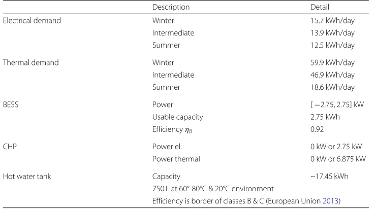
Each configuration is different in terms of constraints and the complexity of determin-ing the set of feasible load profiles: While the BESS is allowed to operate freely within the boundaries of its technical restrictions, the CHP plant’s operation is limited by the tem-perature limits of the connected hot water tank and the household’s heat demand. Hence, to determine the flexibility of the CHP plant, it is necessary to infer changes to the temper-ature of the hot water tank and to determine whether the thermal demand can be satisfied or not. The third configuration is used to evaluate the aggregation of multiple heteroge-neous DERs. Electric and thermal demands in winter, summer, and intermediate seasons, respectively, are determined from the average of 60 simulations of identical households on a weekday using theCREST Demand Model(McKenna and Thomson2016). The sea-sons represent varying consumption patterns and are encoded as three binary variables in the state vector the ANN receives. More detailed information on parameters is given in Table3.

For the evaluation, the model parameters of the DERs are scaled to not exceed±1 kW and the energy demands as well as the hot water tank capacity are scaled accordingly, i.e., divided by 2.75. In practice, this scaling factor (if applied) would be given to the DSMgr

Table 2Data sources for each pattern

Pattern Data Source

A Simulation Model 1a_{and random load profiles}a

B Optimization with objective (2)

C Simulation Model 2

D Simulation Model 1a_{and random load profiles}a

Table 3Overview of model parameters

Description Detail

Electrical demand Winter 15.7 kWh/day

Intermediate 13.9 kWh/day

Summer 12.5 kWh/day

Thermal demand Winter 59.9 kWh/day

Intermediate 46.9 kWh/day

Summer 18.6 kWh/day

BESS Power [−2.75, 2.75] kW

Usable capacity 2.75 kWh

EfficiencyηB 0.92

CHP Power el. 0 kW or 2.75 kW

Power thermal 0 kW or 6.875 kW

Hot water tank Capacity ~17.45 kWh

750 L at 60°-80°C & 20°C environment

Efficiency is border of classes B & C (European Union2013)

alongside the ANNs. The initial states of charge of the BESS and hot water tank range from 0 to 100 % in steps of 10 %. Electricity time-of-use tariffs, which are used in pat-ternB, divide every day into six time slots starting at 06:00, 12:00, 13:00, 17:00, 19:00, and 22:00. Ensuring an average price of 30 cents/kWh throughout the day, the price for every slot is set to either 24, 30, or 36 cents/kWh which leads to 33 possible combinations per day.

Optimization models

Multiple MILPs are employed to evaluate the feasibility of load profiles, to repair infea-sible profiles, and to find the profile featuring the lowest cost. Evaluation and repair are achieved by minimizing the distance to the target load profile. To measure the dis-tance, we use theChebyshev distance L∞, i.e., the maximum absolute difference. The objective is:

min pDraw,pFeedIn

max

k |pDraw,k−pFeedIn,k−pTarget,k| (1)

withpDraw,kandpFeedIn,kbeing the (average) power drawn from or fed into the grid during time slotk. In every slotk, only one of these two non-negative variables is allowed to be positive. The target power during slotkis given bypTarget,k ∈ R. The objective can be linearized by writing the MILP in epigraph form.

In the case of cost optimization, the objective is the minimization of the sum of all energy costs in a given time horizon:

min p·

K

k=0

k·c_Draw,k·p_Draw,k−c_FeedIn,k·p_FeedIn,k+c_Gas,k·p_Gas,k. (2)

All optimization models have either a CHP plant with a hot water tank, a BESS, or both.

Input parametersare the electrical and thermal demands for either summer, winter, or the intermediate seasons, the energy tariffs, the initial state of charge (SoC) of the BESS, and the initial water tank temperature. Theoptimization variablescomprise, aside from some auxiliary variables, the power supplied by the grid, the power feed-in, the BESS (dis-)charge powerpB,k, and binary variables that determine whether the CHP plant is running or not. When calculating the SoC of the BESS, the efficiencyηBis used as follows:

SoC_k+1=SoC_k+k·

⎧ ⎨ ⎩

ηB·pB,k ,pB,k≥0

1

ηB ·pB,k ,pB,k<0

. (3)

Heat losses of the hot water tankpLossHwt,kare given by:

pLossHwt,k=aHwt·

12+5.93+v0.4_Hwt·θHwt,k−θEnv

40 K (4)

using the environmental temperature θEnv, the hot water tank temperatureθHwt,k, and the volume of the tank vHwt in liters. The factoraHwt is set to 1 and hence the heat

loss atθHwt,k = 60◦Cis equal to the boundary between the European space heater effi-ciency classes B and C (European Union2013). To add further constraints and reduce the number of feasible CHP load profiles, we assume that the plant has to keep its state of operation, i.e., being on or off, for at least 15 min which equals the length of 3 time slots. The BESS, on the contrary, is not restricted by such a constraint.

Simulation models

Aside from generating load profiles based on some criterion of optimality by using one of the MILPs, two simulation models are employed to explore further feasible and infeasible load profiles, which are far from being optimal in any sense. In both models, the DERs’ behavior is determined by their internal state, defining how much electricity is consumed or produced and which actions are valid. Once a DER transitions into an infeasible state, e.g., by violating a storage restriction or by keeping a state for too short, a load profile is deemed infeasible. The SoC of the BESS and the thermal losses of the tank are modeled as given in Eqs.3and (4). While the BESS may change its operation mode at any time, the CHP plant has to remain in one mode for at least 15 min. In the simulation, as opposed to the optimization, mode changes may occur at any time and thus are not restricted to the beginning of each 5 min time slot.

Simulation model 1: random behavior

or the CHP plant lead to clear statements about the feasibility of the resulting load pro-files. The simulated and aggregated load of the combination of both, on the contrary, may be incorrectly classified as infeasible. For example, in a simulation run, the BESS could make the invalid choice of exceeding its capacity of 1 kWh by continuously providing 1 kW for more than an hour and thereby invalidate the feasibility of the aggregated profile. The same aggregate, on the other hand, could also be achieved by simply activating the CHP plant and thus may still be feasible. We deal with this issue by evaluating all infeasi-ble schedules of this particular configuration with the MILP introduced above according to the rules derived later in this section.

Simulation model 2: control-vector-based behavior

The purpose of this simulation model is the generation of load profiles for patternC. In this model, the DERs receive a control vector, defining the actions they have to perform in a certain time slot. Essentially, this input vector is an abstract representation of the result-ing load profile. Since the overall feasibility can not be guaranteed for an arbitrary control sequence, either the input has to be classified according to its feasibility or a similar but feasible and thus repaired sequence has to be found. We repair the input vector by mak-ing iterative adaptions, changmak-ing only elements related to time steps up to the time the DER state becomes infeasible. For our tests, we studied two different representations:

1. A control sequence determining the operational mode of the DER for one day in 15 min intervals.

2. Six 4 h time slots in which one mode is activated once for a given time. The representation is the mode and the associated time for every time slot.

The first representation is very similar to an actual load profile and hence closely related to patternD. However, the major difference to patternDis that, here, the repair is achieved using a set of simple rules instead of solving an optimization problem. The second rep-resentation is considered in order to test a more abstract approach. Both reprep-resentations are first attempts and there are many other possibilities to represent load profiles.

Evaluation of load profile feasibility

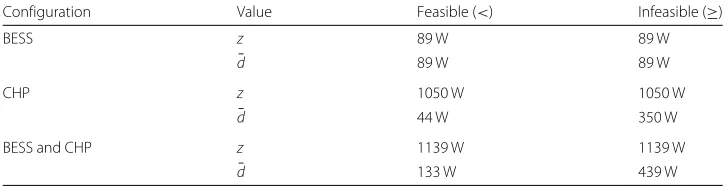
Table 4Thresholds used in load profile evaluation

Configuration Value Feasible (_<) Infeasible (_≥)

BESS z 89 W 89 W

¯

d 89 W 89 W

CHP z 1050 W 1050 W

¯

d 44 W 350 W

BESS and CHP z 1139 W 1139 W

¯

d 133 W 439 W

z: maximum absolute deviation,d¯: average absolute deviation

Profiles that have values ofzandd¯ below the feasibility thresholds are deemed feasi-ble. If at least one of both values is greater than or equal to the respective infeasibility threshold, the load profile is guaranteed to be infeasible. Although there might be indistinguishable load profiles, none occurred in our data.

As opposed to its MILP formulation, the simulated BESS is able to change its mode multiple times within a single time slot. The target power for this slot, which is passed to the optimization, is the average power. Since the optimization solver can decide only once per slot and based on the target power, simply choosing powerpB,k equal to the target powerpTarget,kfor a given slotkmay not be valid. Based on (3) and since we assumed a constant efficiencyηB<1, choosingpB,k=pTarget,kis only problematic when the original load profile requires charging and discharging within the same time slot. In this case, the resulting SoC is lower than the average power suggests1. Depending on the original load profile, the optimized power may have to reproduce the actual SoC by deviating from the target. With regard to the given model parameters, i.e., a (scaled) BESS with a power between -1 kW and 1 kW, this deviation is at most:

−k

2 ·

ηB·1 kW− 1

ηB ·1 kW ≈7 Wh .

This deviation is equal to a 5 min load of 84 W. Adding a margin equal to the optimality gap of 5 % and rounding up leads to the threshold of 89 W forzandd¯(cf. configuration “BESS” in Table4).

ANN design

For each of the usage patterns described in the approach section, the ANN has to rep-resent a specific aspect of the abstracted energy flexibility. These aspects are learnt from examples generated by the models that have been described in the previous sections. We compare instances of the following classes of artificial neural network topologies by how well they are able to internalize the characteristics of the specific models:

(FC) Feed-forward neural networks with fully-connected layers are evaluated as a baseline.

(CNN) Convolutional Neural Networks are evaluated based on the idea that these networks should detect or generate recurring patterns in the load profile.

(RNN) Finally, we exploreRecurrent Neural Networks motivated by the idea that the network should retrace a load profile step-by-step in temporal order, performing a time-discrete simulation of the physical system. We uselong short-term memory

units (Hochreiter and Schmidhuber1997) as recurrent units.

Our main goal is to analyze overall practicability of the proposed approach. That is why we use only a small amount of preferably simple topologies of each class in experiments and do not systematically tune the hyper-parameters of the neural networks. The input data, models, logs, and results are tracked withSacred 0.7.2and published onGitHub(see declaration on data availability for a link). We usedKeras 2.1.1with theTensorFlow 1.4.1

backend to model and train our ANNs.

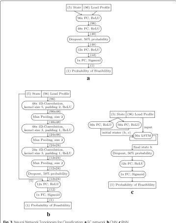
Figure3depicts the evaluated neural networks used for the feasibility classification task and Fig.4shows the neural networks used for the load generation/prediction tasks. Each neural network layer is represented by rounded rectangles and the rectangles represent the input and output vectors. The first number in the layer is the number of neurons or units. The abbreviation “FC” stands for fully-connected layer, “ReLU” is a rectangular lin-ear unit, and “LSTM” is a Long/Short-Term Memory unit (Hochreiter and Schmidhuber

1997). During Up-Sampling, each input vector element is repeated several times.

Training and evaluation methodology

The data sets for each pattern and each combination of DER are pre-generated, shuffled and split into 80 % used for training and validation and 20 % used for the model evalua-tion presented in the results secevalua-tion. For the training of the ANNs, these 80 % are split again into training and validation sets using a ratio of 90/10. In all cases, we use the

Adam optimizerwith the default parameters recommended in (Kingma and Ba2014). The best model of each ANN is selected based on the lowest loss value for the validation data after each epoch. This model is evaluated using the 20 % test data which remains unused for model training/validation. We train all networks with a batch size of 1024 and up to 5000 epochs. The training is stopped whenever the validation loss does not improve in the last 100 epochs (early stopping with 100 epochs patience). Regularization of weights or application of dropout is usually applied to achieve better generalization (Goodfellow et al.2016). We only use dropout in our classification networks.

DER state representation

a

b

c

Fig. 3Neural Network Topologies for Classification.aFC network,bCNN,cRNN

In detail, the state consists of a one-hot-encoded season vector (winter, intermediate, or summer) followed by the state of charge of the CHP plant’s hot water tank and the state of charge of the BESS. If the modeled setup does not contain a CHP plant or BESS, the particular SoC is always set to zero.

For the CNNs and RNNs, applying the convolution or the recurrent time steps on the DER state does not seem plausible. Instead, our classification CNN processes the DER state in layers after the convolution (e.g., see Fig.3a). The CNNs for generating load pro-files process the DER state in the first fully-connected layer (e.g., see Fig.3b). The RNN converts the DER state into initial states of the memory units (e.g., see Fig.3c).

Pattern A: load profile classification

a

b

c

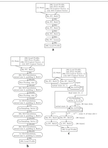
Fig. 4Neural Network Topologies for Load Profile Prediction / Repair.aFC network,bCNN,cRNN

the network represents the probability (or belief )P(feasible)that the given load profile is feasible for the DER in the given state. We use a sigmoid activation function in the output layer and binary cross-entropy as loss function, which is the recommended default for binary classification tasks (Goodfellow et al.2016). We classify a load profile as feasible whenever:

The best performing ANN architectures within our experiments for each topology class are depicted in Fig.3. To be able to compare the topology classes, the architectures are designed so that each topology has approximately 15,000 trainable parameters.

Pattern B: price-based load profile forecasting

In this pattern, the ANN predicts the load profile of the DER for a given price profile and state. We expect the ANNs to generate a 24 h load profile divided into 15 min time slots. Therefore, there are 96 output neurons with linear activation. The loss function used for training is the mean squared error. The expected load profiles are scaled such that the numerical representations remain within the interval [−1, 1].

The ANN topologies for patterns B to D are created based on the classification topologies, where the input data dimensionality is gradually reduced in each layer. The load profile generating ANNs, also, reduce the input data dimensionality to a cer-tain degree, but then increase the dimensionality until the desired number of time slots for the load profile is reached. This way, these topologies resemble autoencoders (cf. (Goodfellow et al.2016)). The resulting topologies are shown in Fig. 4. To be able to compare the three topology classes, the architectures for load prediction are designed such that the number of trainable parameters is approximately 30,000.

Pattern C: load profile generation

In this pattern, the task of the model is to generate a load profile based on a control vector for the DER. Again, the load profiles are scaled to not exceed±1 kW. The data for this pattern is generated using the control-vector-based model described above. The control sequences for the BESS and the CHP plant are divided into 96 slots of 15 min respectively. In addition, we evaluate a second control vector type, where a day is divided into six time slots of 4 h. Each slot contains an operation mode and a duration describing how long the operation mode is active.

Except for the input dimensions of the first layer and an up-sampling factor, the ANN topologies used for this task are essentially the same as those for patternB. First experi-ments have shown that the performance of the RNN benefits from processing the control vector twice.

Pattern D: load profile repair

In this pattern, the ANN receives an infeasible load profile and has to construct a feasible one. Feasible profiles would be filtered beforehand using the classification pattern (i.e., an additional ANN). For our experiments we filtered according to the rules derived earlier in this paper. Both input and output are 24 h load profiles in time slots of 15 min.

We evaluate the same ANN topologies used in patternsBandC and all load profiles are scaled to not exceed±1 kW.

Results and evaluation

Load profile classification

To measure the performance, we use theF1-scoreand accuracy (Goodfellow et al.2016).

TheF1-scorein terms of load profile feasibility is computed fromprecision, i.e., the share

of positively classified profiles that are really feasible, and recall, i.e., the share of all feasible profiles that are positively classified, as follows:

F1=2·precision·recall/ (precision+recall).

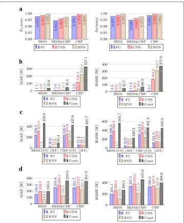
The evaluation results for load profile classification (patternA) are depicted in Fig.5a. The proposed models achieve highF1-scores indicating that a neural network can

distin-guish feasible and infeasible load profiles quite well. In our experiments, however, there was no single best topology for every DER setup. The RNN outperformed the other topologies for the setup with a BESS and the combination of BESS and CHP, whereas the CNN classified CHP load profiles slightly better. Looking at the average scores for each of the three setups, CHP load profiles were distinguished most accurately, whereas classify-ing the load profiles of the BESS/CHP combination was least accurate. One explanation for this result could be the fact that the CHP plant has the strongest operational restric-tions and the BESS/CHP combination has the most degrees of freedom for its operation. The precisions of positive and negative choices for the classification of load profiles of a single CHP plant are similar to those achieved by Neugebauer et al. in (2017).

Preliminary experiments to classify feasibility based on 5 min averages instead of 15 min averages did not improve the general results. We also tested training three independent ANNs, one for each season, instead of encoding the level of thermal consumption in the ANN input. Based on the given input data, there was no general improvement from using three separate ANNs for winter, summer and intermediate seasons. Therefore, we did not pursue this approach any further.

Price-based load profile forecasting

The evaluation results are shown in Fig.5b. As a reference, the average load observed in the training data is determined, which is only one value. The predictor labeled “Const” in Fig.5bpredicts just this average for every time slot. The best results were achieved by a fully-connected network topology.

As can be seen from the mean absolute error (MAE), the predicted load profiles are off by less than 5 W on average, i.e., the absolute error is less than 0.5 % of the scaled power of either the BESS or the CHP plant. We suspect that such good results are achieved by the neural networks that simply memorize a reference load profile for each price profile, as there are only 33 valid price profiles and a load profile may be optimal for multiple input states. In the application context, this behavior is acceptable if the structure of the tariff does not change. If other price profiles are used, the ANN probably needs to be updated.

Load profile generation

a

b

c

d

Fig. 5Results for an ANN with a fully-connected feed-forward topology (FC), a convolutional neural network (CNN), and a recurrent neural network (RNN).aClassification Performance,bLoad Prediction based on Price Profiles,cLoad Generation based on Control Vectors,dLoad Profile Repair (repairing only infeasible profiles)

In general, the models perform better for the battery storage than for the CHP plant. This may be caused by the activation of the plant due to thermal demand, especially for heating in the winter. The thermal demand is a latent variable which the ANN has to infer from the training samples. The BESS, on the other hand, is limited only by the energy storage capacity and the current state of charge.

Load profile validation and repair

very likely that we did not find a suitable topology to solve the task of load profile repair. A fundamental problem may be posed by the fact that repairing an infeasible load profile can be done in many ways. Based on the optimization objective, there may be an infinite number of possible repaired load profiles having the same target function value. Hence, the profiles returned by the optimization are unlikely to follow a systematic scheme. In patternC, on the other hand, the control vector leads to a well-defined load profile. Based on the results of patternC, we expect that ANNs are able to perform better on this task if the profiles are repaired in a consistent and simple way.

Real-world CHP classification

Finally, we tested the best-performing neural network that had been trained for classifying the feasibility of CHP load profiles (the CNN) with real-world data. From a time series, we extracted 51 days from a period that is comparable to the summer state the ANN had been trained with. Based on the measured temperature of the hot water tank, 47 out of the 51 load profiles are correctly classified as feasible. A closer look at the four profiles that were classified as infeasible revealed that they originate from days with very little thermal demand. Hence, the CHP plant that generated these four profiles could not have satisfied the thermal consumption that is assumed in the model and thus the profiles were correctly classified as infeasible.

Conclusion and outlook

In this paper we evaluated the idea of using ANNs as surrogate models for the flexibility of DERs. A major advantage of this approach is that, for a demand side manager, there is no need to explicitly model DERs. In addition, the required amount of communica-tion can be reduced to transmitting a few variables like DER states and prices or load profiles which is a significant advantage with respect to concerns about privacy or data economy.

As our results confirm, the concept of ANN-encoded abstracted flexibilityis indeed viable and there are multiple ways of implementing it. We achieved the best results for the

load profile classification, which we also successfully tested on real-world CHP data, and theprice-based load profile forecastingpatterns. While the mixed results from theload profile generationpattern indicate a general adequacy of the pattern itself, load profile repairdid not work out well for training data generated by the optimization models. Since generation based on a control vector and repair are similar tasks, we conclude that this is likely due to the determinacy of the rules applied in the generation pattern, as opposed to the optimization which generates one of a possibly infinite number of repaired pro-files. Hence, for future evaluations of the repair pattern there should be a well-defined solution.

Endnote

1_{This may be deduced intuitively fromηB<1, (3) and:}

Average Power: pB,k = EB,C,k−_kEB,D,k

Actual SoC: SoCk+1−SoCk = ηB·EB,C,k− _η1_B ·EB,D,k

with total amounts of energy chargedEB,C,kand dischargedEB,D,kduring slotk.

Abbreviations

ANN: Artificial neural network; BESS: Battery energy storage system; CHP: Combined heat and power; CNN: Convolutional neural network; CS: Control sequence; DER: Distributed energy resource; DR: Demand response; DSM: Demand side management; DSMgr: Demand side manager; EMS: Energy management system; FC: Fully-connected; LSTM: Long short term memory; MAE: Mean absolute error; MILP: Mixed integer linear program; ReLU: Rectified linear unit; RMSE: Root mean squared error; RNN: Recurrent neural network; SoC: State of charge; SVDD: Support vector data description

Acknowledgements

The authors would also like to thank the anonymous referees for their valuable reviews and helpful suggestions.

Funding

Publication costs for this article were sponsored by the Smart Energy Showcases - Digital Agenda for the Energy Transition (SINTEG) program. We gratefully acknowledge the financial support from theFederal in Ministry of Education and Research(BMBF) for the projectsENSURE(funding no. 03SFK1A) andKASTEL-SVI(funding no. 16KIS0521) and from the Federal in Ministry for Economic Affairs and Energy(BMWi) for the projectsgrid-control(funding no. 03ET7539G) andC/sells (funding no. 03SIN121).

Availability of data and materials

The data sets generated and used during the current study are available in the Github repository,https://github.com/ kfoerderer/ANN-Encoded-Abstract-Flexibility.

About this supplement

This article has been published as part ofEnergy InformaticsVolume 1 Supplement 1, 2018: Proceedings of the 7th DACH+ Conference on Energy Informatics. The full contents of the supplement are available online athttps:// energyinformatics.springeropen.com/articles/supplements/volume-1-supplement-1.

Authors’ contributions

KF proposed the concept, developed the usage patterns, implemented the simulation models and drafted major parts of the manuscript. MA provided and described the optimization model. KB helped developing the idea, and also designed, conducted and described the ANN implementations and experiments. IM assisted refining the usage patterns, and reviewed the drafts of the manuscript. HS provided feedback, supervision, organization of funding and resources for this collaboration. All of the authors have read and approved the final manuscript.

Competing interests

The authors declare that they have no competing interests.

Publisher’s Note

Springer Nature remains neutral with regard to jurisdictional claims in published maps and institutional affiliations.

Author details

1_{FZI Research Center for Information Technology, Haid-und-Neu-Str. 10-14, 76131 Karlsruhe, Germany.}2_Karlsruhe

Institute of Technology, Institute AIFB, Kaiserstr. 12, 76131 Karlsruhe, Germany.

Published: 10 October 2018

References

Abuella M, Chowdhury B (2015) Solar power forecasting using artificial neural networks. In: 2015 North American Power Symposium (NAPS). IEEE. pp 1–5.https://doi.org/10.1109/NAPS.2015.7335176

Anders G, Schiendorfer A, Steghoefer JP, Reif W (2014) Robust scheduling in a self-organizing hierarchy of autonomous virtual power plants. In: ARCS 2014; 2014 Workshop Proceedings on Architecture of Computing Systems. IEEE. pp 1–8 Batra N, Kelly J, Parson O, Dutta H, Knottenbelt W, Rogers A, Singh A, Srivastava M (2014) Nilmtk: An open source toolkit

for non-intrusive load monitoring. In: Proceedings of the 5th International Conference on Future Energy Systems. e-Energy ’14. ACM, New York. pp 265–276.https://doi.org/10.1145/2602044.2602051

Bremer J, Lehnhoff S (2017) Hybrid Multi-ensemble Scheduling, vol. 10199(Squillero G, Sim K, eds.). Springer, Cham. https://doi.org/10.1007/978-3-319-55849-3_23

Bremer J, Rapp B, Sonnenschein M (2011) Encoding distributed search spaces for virtual power plants. In: 2011 IEEE Symposium on Computational Intelligence Applications In Smart Grid (CIASG). IEEE. pp 1–8.https://doi.org/10.1109/ CIASG.2011.5953329

Callaway DS, Hiskens IA (2011) Achieving controllability of electric loads. Proc IEEE 99(1):184–199.https://doi.org/10. 1109/JPROC.2010.2081652

European Union (2013) Commission Delegated Regulation(EU) No 812/2013 of 18 February 2013 supplementing Directive 2010/30/EU of the European Parliament and of the Council with regard to the energy labelling of water heaters, hot water storage tanks and packages of water heater and solar device Text with EEA relevance. Off J Eur Union 56(L 239):83–135

Faruqui A, George S (2005) Quantifying customer response to dynamic pricing. Electr J 18(4):53–63.https://doi.org/10. 1016/j.tej.2005.04.005

Faruqui A, Sergici S (2010) Household response to dynamic pricing of electricity: a survey of 15 experiments. J Regul Econ 38(2):193–225.https://doi.org/10.1007/s11149-010-9127-y

Förderer K, Ahrens M, Bao K, Mauser I, Schmeck H (2018) Towards the modeling of flexibility using artificial neural networks in energy management and smart grids. In: e-Energy ’18. ACM, New York.https://doi.org/10.1145/3208903.3208915 Gellings CW (1985) The concept of demand-side management for electric utilities. Proc IEEE 73(10):1468–1470.https://

doi.org/10.1109/PROC.1985.13318

Goodfellow I, Bengio Y, Courville A (2016) Deep Learning. MIT Press, Cambridge.http://www.deeplearningbook.org Goodfellow IJ, Pouget-Abadie J, Mirza M, Xu B, Warde-Farley D, Ozair S, Courville A, Bengio Y (2014) Generative

Adversarial Networks. arXiv:1406.2661 [cs, stat]. arXiv: 1406.2661. Accessed 19 Jan 2018

Hinrichs C, Sonnenschein M (2017) A distributed combinatorial optimisation heuristic for the scheduling of energy resources represented by self-interested agents. Int J Bio-Inspired Comput 10(2):69–78.https://doi.org/10.1504/IJBIC. 2017.085895

Hochreiter S, Schmidhuber J (1997) Long Short-Term Memory. Neural Comput 9(8):1735–1780.https://doi.org/10.1162/ neco.1997.9.8.1735. Accessed 16 Jan 2018

Jargstorf J, Jonghe CD, Belmans R (2015) Assessing the reflectivity of residential grid tariffs for a user reaction through photovoltaics and battery storage. Sust Energ Grids Netw 1:85–98.https://doi.org/10.1016/j.segan.2015.01.003 Kingma DP, Ba J (2014) Adam: A Method for Stochastic Optimization. arXiv:1412.6980 [cs]. arXiv: 1412.6980. Accessed 15

Jan 2018

Kochanneck S, Schmeck H, Mauser I, Becker B (2015) Response of smart residential buildings with energy management systems to price deviations. In: 2015 IEEE Innovative Smart Grid Technologies - Asia (ISGT ASIA). IEEE

MacDougall P, Kosek AM, Bindner H, Deconinck G (2016) Applying machine learning techniques for forecasting flexibility of virtual power plants. In: 2016 IEEE Electrical Power and Energy Conference (EPEC). IEEE. pp 1–6.https://doi.org/10. 1109/EPEC.2016.7771738

Malbasa V, Zheng C, Chen PC, Popovic T, Kezunovic M (2017) Voltage stability prediction using active machine learning. IEEE Trans Smart Grid 8(6):3117–3124.https://doi.org/10.1109/TSG.2017.2693394

Mauser I, Müller J, Förderer K, Schmeck H (2017a) Definition, modeling, and communication of flexibility in smart buildings and smart grids. In: ETG-Fb. 155: International ETG Congress 2017. VDE Verlag, Berlin. pp 605–610 Mauser I, Müller J, Schmeck H (2017b) Utilizing flexibility of hybrid appliances in local multi-modal energy management.

In: Proceedings of the 9th International Conference EEDAL’2017 – Energy Efficiency in Domestic Appliances and Lighting. Publications Office of the European Union, Luxembourg

McKenna E, Thomson M (2016) High-resolution stochastic integrated thermal–electrical domestic demand model. Appl Energy 165(Supplement C):445–461.https://doi.org/10.1016/j.apenergy.2015.12.089

Molderink A (2011) On the three-step control methodology for smart grids. PhD thesis. University of Twente.https://doi. org/10.3990/1.9789036531702

Neugebauer J, Bremer J, Hinrichs C, Kramer O, Sonnenschein M (2016) Generalized cascade classification model with customized transformation based ensembles. In: 2016 International Joint Conference on Neural Networks (IJCNN). pp 4056–4063.https://doi.org/10.1109/IJCNN.2016.7727727

Neugebauer J, Kramer O, Sonnenschein M (2015) Classification cascades of overlapping feature ensembles for energy time series data. In: Woon WL, Aung Z, Madnick S (eds). Data Analytics for Renewable Energy Integration. Springer, Cham. pp 76–93

Neugebauer J, Kramer O, Sonnenschein M, van den Herik J (2017) Instance Selection and Outlier Generation to Improve the Cascade Classifier Precision(Filipe J, ed.). Springer, Cham.https://doi.org/10.1007/978-3-319-53354-4_9 Nieße A, Sonnenschein M, Hinrichs C, Bremer J (2016) Local soft constraints in distributed energy scheduling. In: 2016

Federated Conference on Computer Science and Information Systems (FedCSIS). IEEE. pp 1517–1525

Palensky P, Dietrich D (2011) Demand side management: Demand response, intelligent energy systems, and smart loads. IEEE Trans Ind Inform 7(3):381–388

Rodrigues F, Cardeira C, Calado JMF (2014) The daily and hourly energy consumption and load forecasting using artificial neural network method: A case study using a set of 93 households in portugal. Energy Procedia 62:220–229.https:// doi.org/10.1016/j.egypro.2014.12.383. 6th International Conference on Sustainability in Energy and Buildings, SEB-14 Rohbogner G, Fey S, Benoit P, Wittwer C, Christ A (2014) Design of a multiagent-based voltage control system in

peer-to-peer networks for smart grids. Energy Technol 2(1):107–120

Santo KGD, Santo SGD, Monaro RM, Saidel MA (2018) Active demand side management for households in smart grids using optimization and artificial intelligence. Measurement 115(Supplement C):152–161.https://doi.org/10.1016/j. measurement.2017.10.010

Severini M, Squartini S, Fagiani M, Piazza F (2015) Energy management with the support of dynamic pricing strategies in real micro-grid scenarios. In: 2015 International Joint Conference on Neural Networks (IJCNN). IEEE. pp 1–8.https:// doi.org/10.1109/IJCNN.2015.7280621

Toersche HA, Hurink JL, Konsman MJ (2015) Energy management with TRIANA on FPAI. In: 2015 IEEE PowerTech. IEEE. https://doi.org/10.1109/PTC.2015.7232650