Energy-aware test connection assignment for the self-diagnosis of a wireless sensor network

DOI 10.1007/s13173-012-0057-7 L A D C 2 0 1 1

Energy-aware test connection assignment for the self-diagnosis

of a wireless sensor network

Andréa Weber·Alexander Robert Kutzke· Stefano Chessa

Received: 18 October 2011 / Accepted: 13 January 2012 / Published online: 9 February 2012 © The Brazilian Computer Society 2012

Abstract Sensor nodes in Wireless Sensor Networks (WSNs) are prone to failures due to the fragile hardware, malicious attacks, or hostile or harsh environment. In order to assure reliable, long-term monitoring of the phenomenon under investigation, a major challenge is to detect node mal-functions as soon as possible and with an energy efficient approach. We address this problem by using a system-level diagnosis strategy in which the sink issues to the WSN a self-diagnosis task that involves a number of mutual tests among sensors. Based on the test outcomes, the sink ex-ecutes the diagnosis procedure. This work presents an al-gorithm for the assignment of tests among the sensors of a WSN that assures the desired system diagnosability and that is aware of energy consumption. We show by simu-lation experiments that the present approach, as compared to a previous one, enables consistent energy savings on the sensors.

Keywords Wireless sensor networks·System-level diagnosis·Energy-aware·Reliability

A. Weber (

Dept. Informatics Centro Politécnico, Federal University of Paraná, Jdim. Américas, 81531-990 Curitiba, Pr, Brazil e-mail:[email protected]

A.R. Kutzke

e-mail:[email protected] S. Chessa

Institute for Science and Technology of Information, Via G. Moruzzi, 1, 56124 Pisa, Italy

e-mail:[email protected] S. Chessa

Computer Science Department, University of Pisa, Largo Pontecorvo 3, 56127 Pisa, Italy

1 Introduction

A plethora of applications of Wireless Sensor Networks (WSN) [1], including medical diagnosis, infrastructure monitoring, environmental sensing, between others [5,9,16] incur on reliability issues. Corke et al. [9] emphasises the need for software utilities and hardware tools to remotely control and monitor deployed nodes and networks in such a way that slow degradations in transducer performance or battery capacity, for example, are detected and rectified. In this paper, we are concerned with an energy-aware testing approach for identifying node malfunctions in a WSN. As in [28], we adopt asystem-level diagnosisstrategy in which we assume that extreme readings produced by presumable faulty sensors are detected by the sink, which establishes a connection assignment, i.e., that requests the execution of a set of mutual tests in the neighborhood of the nodes under monitoring. The results of such tests are collected by the sink which, in turn, executes a diagnosis algorithm in order to detect the faulty sensors (if any).

Masson [12]; another algorithm able to identify almost all faulty units was later proposed in [4].

Although many system-level diagnosis approaches have been proposed so far [2,3,13,20,23], the fact that the PMC model relies on a central supervisor finds applicability in WSN due to the presence of the sink that can collect and process the diagnostic information.

The present work considers the problem of building a connection assignment of the sensors in a WSN in order to ensure an energy-aware diagnosable system. The PMC model defines a system of n units as t-diagnosable if all faulty units can be diagnosed provided the number of faulty units does not exceedt[19] (tis also called the diagnosabil-ityof the system). In order to diagnosetunits, the following conditions must hold: (c1) the numbernof units in the sys-tem must be greater than or equal to 2t+1, and (c2) a unit must be tested by at leasttother units [19].

The conditions (c1) and (c2) above are necessary and suf-ficient fort-diagnosability provided there are not reciprocal tests, i.e., no two units test each other. On the other hand, if there are units that test each other, a third diagnosability con-dition is formulated in replacement of (c2) [14], for which a corollary is given: (c3) letGbe a digraph of a system of nunits; ifκ(G)≥t then the system ist-diagnosable, where κ(G) stands for the connectivity of G, i.e., the minimum number of vertices whose removal disconnectsG[10].

Specifically, we present an heuristic that chooses the set of sensors to be involved in the tests in order to meet the conditions above. This heuristic, calledEnergy Efficient Test Assignment without reciprocal tests(EETA) builds over our preliminary work [28].

The rest of this work is organized as follows: the next sec-tion presents related work. Secsec-tions3and4present the diag-nostic model and the energy model, respectively. In Sect.5, the energy efficient test strategy is described. In Sect.6, sim-ulation results are evaluated in comparison with a previous approach. Section7presents concluding remarks.

2 Related work

The work of Corke et al. [9] is concerned with outdoor ap-plications of wireless sensor networks involving natural en-vironment or agriculture like microclimate monitoring for farms and rain forests, water-quality monitoring and cat-tle monitoring and control. Nevertheless, the work also ad-dresses the challenges faced by the authors to ensure the reli-ability of the deployed sensors and networks. For soil mois-ture monitoring application, the sensor board includes power supply, solar charging circuit, and sensing for on-board tem-perature, battery voltage and charging current. In rainfor-est monitoring, in the default mode of operation, all energy for the devices come from rechargeable batteries working in

combination with solar panels. In the event no further energy is harvested for long periods, the system switches to non-rechargeable energy supply when the non-rechargeable battery voltage falls below a threshold, and switches back when-ever this voltage rises again. In a lake water quality monitor-ing application, a robot is used to crosscheck the calibration of deployed nodes using its own higher quality temperature transducer in such a way that anomalous events detected by the network are automatically investigated.

In [6], Chessa and Santi present a comparison based test-ing strategy in which the diagnosis model exploits the one-to-many communication paradigm typical of ad-hoc net-works. Both hard and soft faults are considered and the di-agnosis is based upon comparison of the results generated by testing tasks assigned to pairs of units with a common neighbor.

In [27], the problem of determining a connection assign-ment of the sensors in a WSN is considered. Two strategies are shown, one for the scenario in which reciprocal tests among sensors are possible and other for the scenario in which there are no reciprocal tests. In both cases, a square regionR which encloses all sensors that raised an alarm is considered. The testing strategies establish the way the sen-sors in the regionRcoordinate actions to perform the testing tasks. The strategy with reciprocal tests defines that a sensor must test all its neighbors, and considers that the number of sensors in regionR is big enough to reach the desired di-agnosability. In the strategy without reciprocal tests, the re-gionR is partitioned into four quadrants of equal size. Sen-sors present in the same quadrant do not execute reciprocal tests. The sensors in one quadrant ask for tests to the sensors in the successor quadrant and they are asked for tests by the sensors in the predecessor quadrant. Simulations show for which topological properties of the diagnostic graph a desired level of system diagnosability is ensured for both strategies. More details of the approach presented in [27] are shown in Sect.6.

Some works fit the research trend of diagnosis in WSN. In [30], the authors propose a comparison-based fault locat-ing arithmetic for multisource network cluster nodes. The approach is based on layer-built topology structure and one-to-many communication mode. In [8], the authors present a distributed adaptive scheme for detecting faults in WSN where each node makes a local decision based on com-parisons between neighbors, along with the dissemination of the decision to them. Time redundancy is used to en-hance the accuracy of detection and tolerate transient faults in sensing and communication.

faulty sensors can not do any kind of communication. The diagnosis process begins after a fault-free sensor, or an ex-ternal unit, asks for the diagnosis. Thus, the diagnosis works on demand, resulting in an economy of energy for the whole system. The protocol is capable of correct diagnosis in a system with up tot faulty units, wheret < k(G)andk(G) stands for the connectivity of the system. In [24], an energy-efficient distributed approach improves network lifetime by detecting data faults locally in cluster heads. The type of data faults is identified by using trust and reputation con-cepts. The sensors that belong to the same cluster share and compare their readings. From these comparisons, each sen-sor generates a set of possible faulty neighbor sensen-sors. The cluster head verifies which sensors present more fault indi-cations to find the set of possible faulty sensors in the clus-ter. In [25], another energy-efficient cluster-based approach avoids performance degradation aiming at detecting in ad-vance the failures that may cause connectivity loss.

Some other works relevant to ours study topological properties of networks. In [18], a formal proof is presented for the minimum degree a network must have in order to bek-connected with high probability provided the number nof the nodes in the network is big enough. In [29], the au-thors show how many neighbors the nodes of a network with n randomly placed nodes should be connected to in order to the overall network to be connected. The problem of de-termining the critical transmitting range (CTR) for connec-tivity in mobile ad hoc networks is studied in [22]. In this work, Santi investigates the relations between the CTR in case of stationary networks with uniformly distributed nodes and two other cases. The first is the CTR in the presence of M-like node mobility (where M is an arbitrary bounded and obstacle free mobility model) and the second is the case of RWP mobility [15] (which is the most common mobility model used in the simulation of ad hoc networks).

3 Diagnostic model

In our model, we consider a WSN composed of sensors de-ployed in a sensing area with uniform distribution. We as-sume that the topology of the WSN is known to the sink. We also assume that each sensor knows its geographical co-ordinates within the sensing area and that this information is known to the sink. The WSN is modeled as the system graph G=(V , E)where each vertex v inV represents a sensor and an edge(vi, vj)∈Eif and only ifvi andvj ∈V are within the transmission range of each other.

The sensors perform a monitoring task aimed at raising an alarm when they detect anomalous events (for example, in agriculture, the sensors may check for the level of some chemical reactants in a large cultivated area and raise alarms when such level exceeds a given threshold). The alarms are

sent to the sink, which before forwarding the alarm to the user, start a diagnosis procedure to check for their correct-ness. The diagnosis procedure may also be started by the sink on demand or when anomalous readings are reported by a set of sensors. We assume that a setT (of cardinalityt) of sensors have had their readings reported. In response, the sink asks a number of mutual tests among a set of nearby sensorsQ, whereT ⊂Q.

The nature of the test is application dependent; in WSNs, some of the most common causes of failures include sen-sor calibration faults, hardware faults due to harsh environ-ments, connection failures, low battery, between others [26]. In general, a test(vi, vj)consists of a set of input stimuli that are produced by the testing sensorvi and sent to the tested sensorvj. In turn,vj produces a test result that is sent back tovi. Finally,vi compares the output produced byvj with the expected output and it produces the test result that is a binary outcome: it is 0 if the two results match (and then the test succeeds), and it is 1 otherwise (i.e., the test fails). As in the PMC model it is assumed that the outcome of a test per-formed by a fault-free sensor is always reliable (i.e., it is 0 if the tested sensor is fault-free and it is 1 if the tested sensor is faulty), while it is completely unreliable if the testing sensor is faulty. All the test outcomes are finally collected by the sink and decoded by using a suitable diagnosis algorithm.

In the PMC model, the execution of the test requires a bidirectional link betweenvi andvj. However, as observed in [6], in WSN the tests may also be executed in presence of unidirectional links. In particular, a sensor may start a self-test on a predefined set of stimuli and it may send the output to another sensor that compares it with the expected results. Clearly, this second test model does not require a bidirec-tional communication link between the tested and the testing sensors, but it is sufficient only that the tested sensor be able to send its output to the tester. In this paper, we consider tests executed in presence of unidirectional links, and the case in which there are no reciprocal tests. Thus, the diagnosabil-ity can be derived by conditions (c1) and (c2) described in Sect.1.

Our goal is for the sink to define a test connection assign-ment to be used by the sensors to perform the tests. The con-nection assignment is a testing graphD=(VD, ED), where VD⊂V,ED⊂Eand an edge(vi, vj)∈EDif and only if vi testsvj. We definenas the cardinality ofVD.

The heuristic for the definition of the graphDalso seeks for the reduction of the energy consumption needed for the execution of the tests. This is obtained by limiting the num-ber of sensors that take part in the testing procedure. The selection of the sensors ofVD also takes into account their geographical position in order to minimize the distance be-tween the tested and testing sensors. This ensures tests with smaller energy cost.

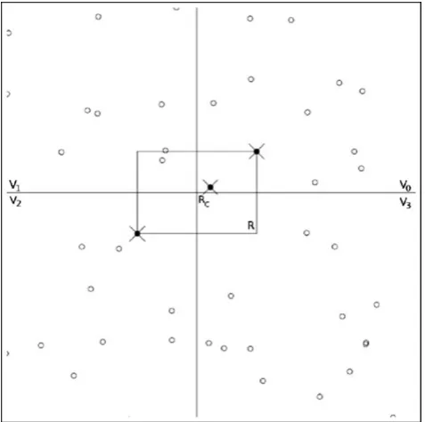
Fig. 1 Network with the definition of the regionR, witht=3

Fig. 2 Example of the division of the network in quadrants usingRc

generated. This region is defined as the smallest rectangular area that comprises all of the sensors inT. Figure1shows an example of the definition of the regionR witht=3. In the figure, circles represent sensors. Sensors shown with an “X” belong toT.

The sensors inV are divided into 4 groups, or quadrants, using the pointRc, the center of regionR, as the basis for the division. Figure2 shows an example of the division of the network into quadrants. We defineVi as the set of sensors

present in quadranti(i=0, . . . ,3). Thus, we haveV =V0∪ V1∪V2∪V3.

Similarly to [27], tests are executed in a predefined order between the quadrants, which ensures that reciprocal tests do not occur. Each quadrant has two neighbors. In a coun-terclockwise order, they are called the predecessor quadrant and the successor quadrant. As opposed to that strategy, in which the sensors seek fort testers between the sensors in the successor quadrant and build the testing graph in a dis-tributed way, in the present strategy the sensors ofVD, de-fined by the sink, execute a predede-fined diagnosis task, whose output is sent to their testing sensors located in the prede-cessor quadrant. These sensors, in turn, send the binary out-come to the sink.

It should be observed that, in order for the diagnostic graphDto bet-diagnosable, the conditions (c1) (i.e., that n≥2t+1) and (c2) (i.e., the indegree of each vertex inDis at leastt, or, in other words, each sensor is tested by at least tother sensors) should be met [19].

4 The energy model

In order to estimate the energy consumption of a given testing assignment, we consider the one-slope model [17], a widely used propagation model in wireless communica-tions. This model assumes a linear dependence between the path loss (dB) and the logarithm of the distance d between the transmitter and the receiver, as expressed in1:

L(d)|dB=l0+10αlog10(d) (1)

wherel0 is the path loss at a reference distance of 1 me-ter (though the paper we express distances in meme-ters), and αis the power decay index (also called path loss exponent). In general, to ensure a communication between a transmit-tert and a receiverr placed at distance d from each other it is necessary that the packet sent by t reaches r with a power level higher than the sensitivity of the receiver. In other words, letting Et be the transmission power of the transmitter,Erthe power of the signal at the receiver (where Erdepends onEtand the distanced), and Em be the sensi-tivity of the receiver, must beEr> Em.

By (1) must be

Er=

Et

10(l0+10αlog10(d)) (2)

IntroducingEr > Emin2, we obtain that the minimum transmission powerEtat the transmitter that ensures that the packet reaches the receiver with the required power is

Now (3) depends on the distanced, the sensitivity of the receiver and the parametersl0andα. For the latter param-eters, we take in the simulations typical values [21] (in par-ticular, we setl0=10 andα=3), whileEmdepends on the actual hardware of the WSN.

From (3), it follows that the energy spent grows polyno-mially with the distanced, with an exponent equal toα.

5 The energy efficient testing strategy

The Energy Efficient Test Assignment without reciprocal tests (EETA) algorithm builds the testing graphD by tak-ing into account the total energy cost needed for the sensors to execute all the tests of the connection assignment. To this purpose, EETA definesCi,j as the energy cost spent by the sensorsvi andvjwhen the sensorviexecutes a test over the sensorvj.

Initially, EETA initializes setVD as the set of sensors in regionR. Considering the division in four quadrant of the WSN, alsoRresults divided in four quadrants accordingly. As a result also the sensors in setVDcan be considered split into four subsets, each corresponding to a quadrant. Specif-ically, we defineQi (with 0≥i≤3)as the set of sensors positioned in quadrantiand selected for the connection as-signment. Thus, we haveVD=Q0∪Q1∪Q2∪Q3, with Qi⊂Vi.

In order to satisfy the conditions stated in Sect.3, each of theQimust be composed of at leasttsensors (with the sen-sors ofT included). Witht sensors in each quadrant, each sensor can be tested byt others(c2)and the number of sen-sors that participate to the diagnosis is sufficient to satisfy (c1), once we have 4t≥2t+1. As long as the testing strat-egy tries to diminish the number of sensors inVD, we have n=4t, the minimumn required in our heuristic. Further-more, the distance toRc, the center of regionR, is also taken into account to choose the sensors inVD.

Note that the initial selection ofVDmay not be sufficient to ensure thatt sensors per quadrant are chosen, hence, in this case, other sensors outsideR should be added toVD. However, in cases where the regionR is near the border of the network, it may not be possible to have at least t sen-sors in each quadrant. In order to guarantee the number of testers per quadrant, the centerRc of the regionR is then shifted toward the center of the network andR is enlarged accordingly.

The total energy cost spent by the tests made by the sen-sors present in quadrant i is defined as CQi, i.e., CQi =

Ci,j ∀(vi, vj)∈ED|vi ∈Qi andvj∈Q(i+1)mod 4. We also define the total energy cost spent by all tests made by D asCT(D). Thus, we haveCT(D)=

3

i=0CQi. The

se-lection of sensors ofVDis made to minimize the total energy consumption by tests between sensors.

For the diagnosis to be possible, condition(c2)must be fulfilled. As|Qi| =t, we can conclude that a sensorvk ∈ Qi will test all sensors present in Q(i+1)mod 4, i.e., ED= {(vk, vl)∀vk∈Qi and∀vl∈Q(i+1)mod 4fori=0, . . . ,3}.

It should be observed that edge(vi, vj)∈EDmay not ex-ist initially inE, i.e., the sensorvi may not be on the trans-mission range of the sensorvj. In order to make possible that the sensorvi testsvj it is necessary that the transmis-sion range ofvj be tuned. So the sink asks the sensors that are not neighbors of their testing sensors, i.e., that make and edge inED, to augment their transmission ranges (i.e., the transmission power) in order to enable the test. The underly-ing assumption is that the network is dense and large andtis relatively small with respect to the network density so that the cases in which a sensor must augment its transmission power is unlikely to happen.

In order to permit that the selection of sensors in each quadrant makes the reduction of CT(D) possible, an ini-tial heuristic is used. At first, the sensors inT are selected for each of the quadrants in which they are positioned, since those sensors must participate to the testing procedure. Thus, we define Ti as the set of sensors of T geographi-cally positioned in quadranti. The cardinality ofTi is equal toti. Thus, we haveTi ⊂Qi and

3

i=0ti =t. Consider-ing the energy model presented in this work, the energy cost needed for the execution of a test grows polynomially with the geographic distance between the sensors. Thus, if sen-sors that are geographically near are selected for VD, we have a higher probability of generating a testing graphD with a value ofCT(D)that is reduced.

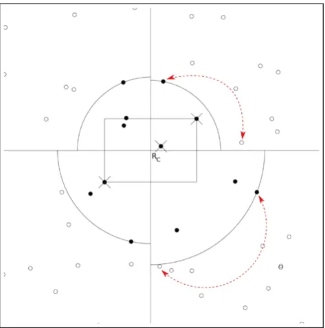
The initial selection of sensors inVD is thus based on the distance of the sensors to a common point,Rc in this case. Based on this principle,Qi is initially formed by the ti sensors ofTi and thet−ti sensors of the quadranti geo-graphically nearer fromRc. Thus,VD is formed mainly by sensors near toRc. Figure3shows an example of the def-inition of the setVD. Black bullets represent sensors that belong toVD. It should be observed that the simple strategy of picking up any initial set oft sensors does not lead to an optimal solution.

Even though the initial heuristic has the goal of selecting the nearest sensors to the pointRc, it should be observed that a sensorvk∈Ti may be farther fromRcthan a sensorvl∈ (Vi−Qi). Nevertheless, every sensorv∈T must participate to the diagnosis procedure, regardless of its distance to the pointRc.

Fig. 3 Definition of the initial setVDwith the sensors ofT (marked

with an “X”) and the sensors geographically nearest fromRc, with t=3

Fig. 4 Example of choice of sensor farther fromRcwith lower energy

cost

sensors in the neighbor quadrants may diminishCT(D). In order to evaluate the possible sets of sensors that guarantee a minor value for CT(D) than that obtained by the initial heuristic, an algorithm is executed.

Consider the sensorsvk∈Vi andvl∈Vi. The sensorvk is defined as the sensor farthest fromRcthat belongs toQi, andvl is defined as the sensor geographically nearest to the

Fig. 5 The network after the exchange of the sensors that participate to the testing graphD

sensorvk, and farther fromRc thanvk, so thatvl∈/Qi. In other words,vl is the sensor nearest fromRc that was not selected forQi. The algorithm consists in verifying if the exchange of any sensorvn∈Qiby the sensorvl produces a reduction inCT(D). The exchange that produces the higher reduction inCT(D)is performed. The process is repeated searching for other possible exchanges and is finished once the exchange of a sensorvn∈Qi by any sensorvl∈/Qi does not generate a reduction inCT(D).

This process is performed in all of the quadrants, one quadrant at a time, i.e., at first the possible exchanges are verified in quadrant 0, until no exchange is performed, then the process is initiated in quadrant 1, and so on. The strat-egy is finished when there is no exchange in any of the four quadrants.

Although the quadrants may be visited more than once in the searching for possible exchanges, the strategy is fi-nite once at some point every farther sensor will produce a higher cost. It is also clear that this heuristic iterates at most a number of times equal to the number of the sensors in the network.

6 Evaluation

(Test Assignment Without Reciprocal tests), and the EETA heuristic.

TAWR [27] divides the region R into four quadrants. Sensors of a quadrant ask for tests for sensors on the suc-cessor quadrant and test sensors on the predesuc-cessor quad-rant. Thus, the sensors themselves define the testing graph. Furthermore, the test procedure is not based on a self-test as in EETA, which produces greater information exchange be-tween the sensors and thus greater overhead. More specifi-cally, in TAWR each node asks for tests broadcasting a mes-sage seeking for testers. Sensors in the neighbor quadrant that receive the messages answer sending testing stimuli. Then the tested sensors send test replies to the testers. Thus, the overhead is greater than that of EETA, in which the sink defines the testers of each node and the tested sensors send replies to a predefined set of testing stimuli.

In all of the simulations, networks of size 100×100 m2 composed of 512 and 1024 sensors are considered. For each simulation experiment, a region with 10% of the total size of the network is randomly defined.t sensors of this region are randomly selected as the sensors ofT. Experiments were run for the following values oft: 5, 8, 10, 12, and 15.

For each set of input values, a set of 100 different random network graphs were generated. For each graph, the simu-lator creates the diagnostic graphD and calculates the en-ergy costCT(D), based on the models presented in Sects.4 and5.

In EETA, the cost of a test executed by sensorvi on sen-sor vj at a distanced from each other is computed as the sum of the energy spent byvj to send the output sequence of a self-test to vi, and by vi to receive such outcome. In particular, for each packet sent we consider (3) instantiated with typical values of class mote sensors, taken from their datasheets [11], and we make the assumption that each test involves 100 packet’s transmissions.

In TAWR, the testing links are bidirectional, as in the tra-ditional PMC model. Thus, the cost of a test executed by sensor vi on sensor vj is equal to the sum of the energy spent sending a test task from sensorvi to sensor vj plus the test reply by the tested sensorvj back to sensorvi. As opposed to the results presented in [28], in which only the cost of sending an output test sequence was computed for comparison with EETA, in the present work the overall cost of TAWR is taken into account for comparison purposes.

Four sets of experiments were run. Figure 6 shows the ratio between the total energy costCT(D)consumed by the tests of graphDof both strategies, and for different values of t. Not surprisingly, the strategy EETA presents smaller CT(D) in all simulation experiments, either on networks with 512 sensors or on networks with 1,024 sensors.

Furthermore, the algorithm of strategy EETA employs a smaller number of sensors in the diagnosis process. Thus, less tests are performed, generating smaller total energy

Fig. 6 Ratio between the total energy cost presented by strategies EETA and TAWR, for different values oft

Fig. 7 Number of sensors used by strategies EETA and TAWR, with different values oft

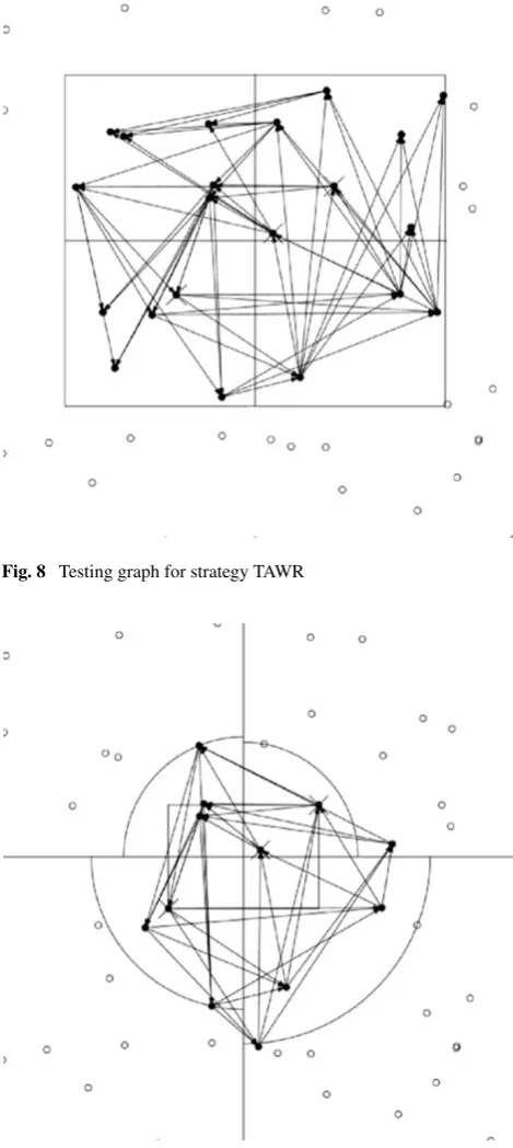
costsCT(D). TAWR uses more thantsensors in each quad-rant; astsensors are needed for each sensor that participates in the diagnosis that makes n >4t in that heuristic. Fig-ure7 shows a comparison between the number of sensors used in the diagnosis process in both strategies. For strategy EETA, a number of 4t sensors is always used. For strategy TAWR, on the other hand, the number of sensors used in the diagnosis process increases with the network density. Even though the increase in the network density ensures tests with a smaller cost in both strategies, the use of a greater num-ber of sensors increments the total energy cost in strategy TAWR. It should be observed that in Fig.7 the results of strategy EETA for 512 sensors and for 1,024 sensors are overwritten, once they are the same (4t), i.e., strategy EETA always uses the minimum number of sensors in the diagno-sis process. Figures8and9show the testing graphs gener-ated in each strategy for the same set of initial nodes under monitoring. It should be observed that the number of sen-sors used by EETA is reduced if compared to the number of sensors used by strategy TAWR.

num-Fig. 8 Testing graph for strategy TAWR

Fig. 9 Testing graph for strategy EETA

ber of sensors used in the diagnosis process. Similarly to the total energy costCT(D), the average cost is also smaller for strategy EETA.

The strategies have their maximum costs compared in Fig. 11. The maximum energy cost used by one strategy, CM(D) is equal to the energy consumption presented by the sensor with maximum cost, i.e., between all of the sen-sors that participate to the process, the sensor with

high-Fig. 10 Ratio between the average energy cost presented by strategies EETA and TAWR, for different values oft

Fig. 11 Ratio between the maximum energy cost presented by strate-gies EETA and TAWR, for different values oft

est energy consumption is chosen. The cost of this sen-sor is then named the maximum cost ofD. Thus, we have CM(D)=max(Ci∀vi∈VD), whereCi is the total cost pre-sented by the sensorvi. Again, EETA performs better than TAWR.

7 Conclusion

the energy cost of a test between sensors grows polynomi-ally with the distance between them.

Experimental results show that EETA presents total, av-erage and maximum energy costs smaller than TAWR. Fur-thermore, EETA applies a smaller number of sensors than TAWR. Future work includes simulation experiments to evaluate the scalability of the solution presented, and the comparison with other energy-efficient approaches. We also plan to investigate the fairness in the energy consumption of the sensors, and strategies that assign testing tasks to sensors with more residual energy.

References

1. Baronti P, Pillai P, Chook VWC, Chessa S, Gotta A, Hu YF (2007) Wireless sensor networks: a survey on the state of the art and the 802.15.4 and ZigBee standards. Comput Commun 7:1655–1695 2. Barsi F, Grandoni F, Maestrini P (1976) A theory of diagnosability

without repair. IEEE Trans Comput C-25:585–593

3. Bianchini RP, Buskens RW (1992) Implementation of on-line distributed system-level diagnosis theory. IEEE Trans Comput 41:616–626

4. Caruso A, Chessa S, Maestrini P (2007) Worst-case diagnosis completeness in regular graphs under the PMC model. IEEE Trans Comput 56(7):917–924

5. Chen G, Hanson S, Blaauw D, Sylvester D (2010) Circuit design advances for wireless sensing applications. Proc IEEE 98(11):1808–1827

6. Chessa S, Santi P (2001) Comparison-based system-level fault di-agnosis in ad-hoc networks. In: Proc IEEE SRDS 2001, Sympo-sium on Reliable and Distributed Systems, Oct, pp 257–266 7. Chessa S, Santi P (2002) Crash faults identification in wireless

sensor networks. Comput Commun 25(14):1273–1282

8. Choi J, Yim S, Huh YJ, Choi Y (2009) A distributed adaptive scheme for detecting faults in wireless sensor networks. WSEAS Trans Commun 8(2):269–278

9. Corke P, Wark T, Jurdak R, Hu W, Valencia P, Moore D (2010) Environmental wireless sensor networks. Proc IEEE 98(11):1903– 1917

10. Cormen TH, Leiserson CE, Rivest RL, Stein C (2001) Introduc-tion to algorithms. MIT Press, Cambridge

11. Crossbow Technology Inc.http://www.xbow.com

12. Dahbura AT, Masson GM (1984) An O(n2.5_{) fault} identifica-tion algorithm for diagnosable systems. IEEE Trans Comput C-33:486–492

13. Duarte EP Jr., Nanya T (1998) A hierarchical adaptive distributed system-level diagnosis algorithm. IEEE Trans Comput 47(1):34– 45

14. Hakimi SL, Amin AT (1974) Characterization of connection as-signment of diagnosable systems. IEEE Trans Comput C-23:86– 88

15. Johnson DB, Maltz DA (1996) Dynamic source routing in ad hoc wireless networks. In: Mobile Computing, pp 153–181

16. Ko P, Lu C, Srivastava MB, Stankovic JA, Terzis A, Welsh M (2010) Wireless sensor networks for healthcare. Proc IEEE 98(11):1947–1960

17. Patwari N, Hero AO, Perkins M, Correal NS, O’Dea RJ (2003) Relative location estimation in wireless sensor networks. IEEE Trans Signal Process 51(8):2137–2148

18. Penrose MD (1999) On k-connectivity for a geometric random graph. Random Struct Algorithms 15:145–164

19. Preparata F, Metze G, Chien RT (1968) On the connection assign-ment problem of diagnosable systems. IEEE Trans Electron Com-put 16:848–854

20. Rangarajan S, Dahbura AT, Ziegler EA (1995) A distributed system-level diagnosis algorithm for arbitrary network topologies. IEEE Trans Comput 44:312–333

21. Rappaport TS (2001) Wireless communications: principles and practice, 2nd edn. Prentice Hall, New York

22. Santi P (2005) The critical transmitting range for connectivity in mobile ad hoc networks. IEEE Trans Mob Comput 4(3):310–317 23. Subbiah A, Blough DM (2004) Distributed diagnosis in dynamic

fault environments. IEEE Trans Parallel Distrib Syst 15(5):453– 467

24. Taghikhaki Z, Sharifi M (2008) A trust-based distributed data fault detection algorithm for wireless sensor networks. In: 11th interna-tional conference on computer and information technology, Dec., pp 1–6

25. Venkataraman G, Emmanuel S, Thambipillai S (2008) Energy-efficient cluster-based scheme for failure management in sensor networks. Commun, IET 2(4):528–537

26. Wang X, Ding L, Wang S (2011) Trust evaluation sensing for wire-less sensor networks. IEEE Trans Instrum Meas 60(6):2088–2095 27. Weber A, Kutzke AR, Chessa S (2010) Diagnosability evaluation

for a system-level diagnosis algorithm for wireless sensor net-works. In: IEEE symposium on computers and communications, Riccione, Italy, pp 241–244

28. Weber A, Kutzke AR, Chessa S (2011) Energy-aware test connec-tion assignment for the diagnosis of a wireless sensor network. In: Fifth Latin-American symposium on dependable computing, São José dos, Campos, Brazil, pp 65–73

29. Xue F, Kumar PR (2004) The number of neighbors needed for connectivity of wireless networks. Wirel Netw 10(2):169–181 30. Zhang J, Jing B, Sun Y (2008) Fault locating arithmetic for