How to evaluate the reliability
of regional input–output data? A case for China
Haoyang Zhao
*, Jian Xu and Xinteng Liu
1 Background
Economic research has been increasingly concerned with structural issues and value-added in multi-sector international trade. Therefore, input–output (IO) data have become a prevalent data source and been more frequently used in empirical analyses. As a result, the accuracy and reliability of IO data raise serious concerns since the credible data ensure credible empirical results. In fact, there has been ample research dedicated to the quality of government statistics (Zhao et al. 2011). It turns out that no socioeco-nomic statistical data are completely precise due to statistical regime defects (Xu 1994; Jin and Tao 2010; Holz Holz 2013a, b), investigation and aggregation errors (Park and Wang 2001; Agafiţei et al. 2015) and lack of independence in statistical agencies (Outrata
2015). It is reasonable to presume that IO statistics, as a type of government statisti-cal data, also suffer from some similar quality issues. Thus, the core problem is how to assess the accuracy and quality of current IO data.
There has been a prolonged history of using IO data in government statistics. As a part of national accounting, input–output first appeared in A System of National Accounts
(SNA1968; United Nations 1968). Then, in System of National Accounts 1993 (SNA1993;
Abstract
Accurate statistical data are essential to a credible and cogent empirical analysis. How-ever, there currently is no mature and specialized methodology to evaluate the accu-racy of input–output (IO) data. This research constructs a comprehensive yet relatively concise framework for evaluating the accuracy of regional IO data by including several indicators that measure all three quadrants. The framework examines regional IO data from the perspectives of time consistency and variation, coefficient correlation and its homogeneity with national-level data. A score indicating the overall accuracy and detailed information that presents concrete shortcomings of regional IO data could be offered after analysis using this framework. As an example, the provincial-level IO data for 30 provinces for 3 years (2002, 2007 and 2012) are analyzed by this framework, and possible explanations of the results are offered. The main contribution and innovation of this research is the construction of an applicable and exhaustive quality evaluation framework for regional IO data. This framework enables researchers to realize flaws in IO data before utilizing them. It also allows government agencies to improve the quality of their data by avoiding issues that emerged in previous data quality evaluations. Keywords: Data quality, Quality evaluation, China, Regional IO data
Open Access
© The Author(s) 2017. This article is distributed under the terms of the Creative Commons Attribution 4.0 International License (http://creativecommons.org/licenses/by/4.0/), which permits unrestricted use, distribution, and reproduction in any medium, provided you give appropriate credit to the original author(s) and the source, provide a link to the Creative Commons license, and indicate if changes were made.
RESEARCH
*Correspondence: haoyangzhaoruc@outlook. com
United Nations et al. 1993), the non-investigative supply-use table was introduced, and IO data were considered a major component of national accounting. In System of National Accounts 2008 (SNA2008; European Commission et al. 2009), IO tables were considered an extension of production accounts. Furthermore, SNA2008 recommends a supply-use table framework instead of survey-based IO tables since supply-use tables are much easier to acquire, which could enable statistical agencies to release IO table more efficiently and frequently. Two specific IO manuals, UN (1999) and Eurostat (2008), guide the compilation of IO tables. In terms of regional IO data, Miller and Blair (2009) present how to apply several non-survey methods, such as RAS, to compile regional IO tables, and offer theoretical regional models as well.
Before implementing evaluations, standards respecting statistical quality need to be specified. International organizations have long possessed major concerns over the stand-ards for statistical data. The first organization that paid attention to the quality of statisti-cal data was the UN in 1980. Different from other organizations, the UN (2003) primarily focused on optimizing the structure of statistical agencies, arguing that these agencies should obtain independence, relevance, credibility and respondent policies as their foun-dations. The IMF (2013a, b) required all subscribers of the Special Data Dissemination Standard (SDSS) to follow four statistics criteria. First, the data must have ample cover-age, periodicity and timeliness. Second, the data must be publicly accessible. Third, the data and the process must possess integrity. Fourth, the data must have proper quality, meaning the methodology and data must be reasonable and pass cross-checking. The General Data Dissemination Standard (GDDS) was also released by the IMF (2013a, b). It is designed for relatively less-developed government statistical systems but shares the same general requirements. OECD and Eurostat provide more detailed standards than those previously discussed in this paragraph. The OECD (2011) measures statistical data from eight dimensions, including accuracy, coherence, timeliness and accessibility, among others. Eurostat (2011) presents a method that is constituted by 15 principles that cover the institutional environment, the statistical production processes and the output of statistics. This process is aimed at ensuring accurate, coherent and comparable data. Outside of organizations, individual researchers have also established several data quality standards that address data accuracy, timeliness and availability (Brackstone 1999).
All data quality evaluation methods are classified into two branches: data-driven and theory-driven. Data-driven methods are based on the data itself, only use statistics, mainly focus on finding outliers in a group of data points and determine the data quality by the number of outliers. For instance, Zhang (2003) introduces a statistical test to find outli-ers by assuming that the data distribution is exponential. Another example comes from machine learning, which offers various algorithms (such as support vector machines) that can be used to separate outliers from the remaining points (James et al. 2014).
time-series analysis or simple comparisons (Sinton 2001). Different from these methods that are based on the calculations of real data, Wang and Jin (2010) created a question-naire that included measurements of respondents’ subjective impressions of the quality of statistics.
Several conclusions can be drawn from the research discussed above. An apparent issue is that none of this research is IO specific. The majority concentrate on GDP, and the remaining study transportation, energy and other particular areas other than input– output data. A derivative problem is that, although standards or principles remain the same, these methods are only compatible with simple statistical indicators that reflect an economic scale. However, IO data consist of hundreds of interrelated statistics that con-currently demonstrate economic scale and structure. The delicate correlations between data indicate that a systematic method or framework needs to be established to evaluate the quality of IO data.
Therefore, the main contribution of this paper is to construct a plausible framework to evaluate regional IO data. The reason that we assess regional instead of national data is that a benchmark is necessary during evaluation. National data are usually of better quality and more consistent, making it more appropriate as the benchmark.
To be precise, not all the principles of statistical data mentioned above will be imple-mented in the following IO data analysis. Since the objective of this paper is to evaluate the quality of data, standards such as data availability that measure the quality of statisti-cal agency services instead of the data itself are omitted. Additionally, standards that are not applicable to IO data, such as coverage, are also omitted. The standards measured in this paper are data accuracy, coherence between regional and national data, and time-series consistency.
The remainder of this paper is arranged as follows: In Sect. 2, a framework evaluat-ing regional IO data as a whole and individually is constructed. Section 3 is the empiri-cal analysis that uses the framework constructed in Sect. 2 and applies the framework to China. Section 4 offers possible explanations of the results. Section 5 concludes the work.
2 Constructing the evaluation framework
An IO table consists of hundreds or thousands of interrelated numbers. This large quan-tity of data could be highly favored by scholars and policy makers. Nevertheless, it may lead to more difficulties when compared to the evaluation of the quality of single-num-ber data, like CPI, since it is not possible to find reference indicators outside the IO table for every single number. Therefore, when constructing the evaluation framework, two premises have been set as follows.
(1) The source of data used in an evaluation is the regional and national IO data only. (2) Only limited but representative data will be involved in the analysis of IO data
qual-ity. Specifically, relatively important (and large enough) direct input coefficients or key coefficients (KC) will be representative numbers.
input–output data is a data system constituted by multiple input–output matrices, and every matrix is composed by the same bundle of sectors, it is natural to measure the data quality using the regional and industrial angles. The regional angle examines whether there are significant differences in data quality between individual regions. The industry angle examines whether the data quality of some industry is questionable, regardless of the region. As we previously stated, for direct input coefficients, it is more desirable to examine only key coefficients, which achieves a balance between the evaluation accuracy and time costs. In terms of the final demand and value-added, due to the relatively small number of cells, all data could be assessed. Then, several indicators are constructed according to the IO and economic theories, which includes concerns about the consist-ency and coherconsist-ency of the individual data table and the entire data system. The ration-ales for indicators are explained below. The final step is to summarize all those indicators to evaluate the quality of different regions and sectors.
Now we can begin the construction of the evaluation framework. It is reasonable to construct an indicator using the ratio of the number of aberrant KC(s) to the number of all KCs. A higher ratio indicates a lower-quality IO table. Likewise, it can also be used to examine the IO data quality in a certain sector or even data of all regions as a whole (national IO data system).
Next, it is critical we define aberrant KC(s). From IO theory, direct input coefficients (as symbols of production technology) remain stable at least in short terms. Hence, once a mutation occurs, a zero KC turns into a significant nonzero one in the next year, or, vice versa, this KC is categorized as aberrant. The term “mutation” implies that these kinds of changes usually indicate a technological revolution in production, and new sec-tors emerge, or old secsec-tors die. Any of these changes can be regarded as so tremendous that it is highly unlikely they occur in a short time period. Nevertheless, KCs do not retain absolute stability, and minor changes are inevitable between two accounting years. However, those changes are neither random nor without constraints. An assumption is that these changes follow similar features or trends for KCs within a sector, since the same national macroeconomic and industry policies and similar market and technology conditions are shared by all KCs in a certain sector regardless of the region. Accordingly, if some change(s) of KC(s) become outliers of all changes, these KC(s) are also consid-ered as aberrant.
In summary, we need to stress that not all changes are viewed as quality flaws. Instead, only drastic, irregular changes are treated as errors and mistakes. These changes are far from those caused by normal disturbances and are highly unlikely to be explained by minor issues such as price differences or random errors.
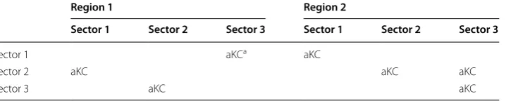
A simplified example is shown below to more clearly illustrate aberrant KC indicator. Assume we have a nation with two regions and three sectors. By some method, eight direct input coefficients have been confirmed as KCs, including all direct input coeffi-cients except a12. The locations of aberrant KCs are given in Table 1, and the number of aberrant KCs is displayed in Table 2.
Note that when counting the number of sectors, if amn is a KC, it is treated as a KC in both sectors m and n. If m=n, amn is treated as 2 KCs in sector m (n).
Therefore, the KC indicators are calculated as follows.
Coherence in each sector and all regions also need to be taken into consideration. From the analyses above, evaluations for individual regions compare data from different years to draw conclusions. Therefore, evaluations must use a data package that includes 2-year datasets and concurrently displays the results of 2 years together. However, as for each sector and all regions together, national data serve as a benchmark, and results of single years are available.
To utilize national-level statistics as benchmarks, a new indicator is introduced. A sim-ple character of a coherent data system is the aggregation of regional-level data approx-imately equal to the national data. Accordingly, a ratio of the aggregation to national data is a reasonable measurement, which accounts for total output, consumption, capital
Ratio of KC
Region 1
=3/8=0.375
Ratio of KC
Region 2
=4/8=0.500
Ratio of KC (Sector 1)=(2+2)/(5+5)=0.400
Ratio of KC (Sector 2)=(2+3)/(5+5)=0.500
Ratio of KC(Sector 3)=(2+3)/(6+6)=0.417
Ratio of KC(Nation)=(3+4)/(8+8)=0.438
Table 1 An example of locations of aberrant KCs in an imaginary nation
a Aberrant KCs are marked by notation aKC
Region 1 Region 2
Sector 1 Sector 2 Sector 3 Sector 1 Sector 2 Sector 3
Sector 1 aKCa aKC
Sector 2 aKC aKC aKC
Sector 3 aKC aKC
Table 2 An example of the number of aberrant KCs in an imaginary nation
Region 1 Region 2
The number of aberrant KCs 3 4
In sector 1 2 2
In sector 2 2 3
formation, labor compensation and other indicators. If the ratio of a sector significantly deviates from 1, the data of the sector is incoherent since the data contradict other data. Thus, the ratio of incoherent sectors (IS) to all data is a proper indicator aimed at the data quality of each sector and all regions together. Similarly, the aggregation of total inward flows and outward flows (goods and services imported from/exported to other region but not from/to foreign countries) should be approximately equal. If the ratio of the aggregation of inward flows to one of outward flows is significantly larger or smaller than 1 certain sector, this sector needs to also be treated as IS.
Here is an example illustrating this indicator. Suppose again that a nation has three sectors and IS data are identified and noted in Table 3.
Therefore, the IS indicators are calculated as follows.
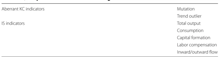
To sum up, Table 4 demonstrates the quality evaluation framework for the regional IO data established above.
The data quality of each region is given by aberrant KC indicators, while the quality of each sector and the whole nation is the average of the individual aberrant KC indicator and IS indicator.
For example, the data quality of the imaginary nation in the example above is 0.419.
Ratio of IS(Sector 1)=2/5=0.400
Ratio of IS(Sector 2)=3/5=0.600
Ratio of IS(Sector 3)=1/5=0.200
Ratio of IS(Nation)=(2+3+1)/15=0.400
(0.438+0.400)/2=0.419
Table 3 An example of IS indicator in an imaginary nation
a Incoherent sectors are marked by notation IS
Sector 1 Sector 2 Sector 3
Total output
Consumption ISa IS
Capital formation IS IS
Labor compensation IS
Inward/outward flow IS
Table 4 Quality evaluation framework for regional IO data
Aberrant KC indicators Mutation
Trend outlier
IS indicators Total output
3 Evaluation of province‑level IO data in china
In this section, in order to apply the established framework, China’s provincial-level IO data are analyzed.
3.1 Data
The IO accounting years in China end with 2 or 7 (based on real IO survey) and 0 or 5 (updated using general national accounting data). IO data in the most recent three con-secutive accounting years based on the real survey (2002, 2007 and 2012) constitute the data source. The evaluation includes all provinces in mainland China except Tibet. In short, 30 provincial-level tables in 3 years (90 total tables) are included. In addition, the national IO table in these years is used for benchmarks. All data are available from the National Bureau of Statistics of China (NBS).
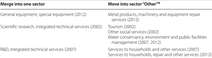
All tables used here contain 42 sectors. However, there are some minor changes in sector classifications between any 2 years. Therefore, sector adjustments have been implemented to keep the sector classification consistent over time, and the adjustment procedures are listed in appendix (Tables 9, 10 for the result of adjustments). Therefore, all tables are modified into a 39-sector version. Specific changes on sectors and sector classifications after adjustments are listed in appendix.
3.2 Aberrant KC indicators
3.2.1 Choose key coefficients (KCs)
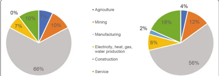
It is true that there are several methods to choose KCs. However, to simplify the calcu-lation, a single rule has been adopted for choosing KCs such that if amn is larger than 0.05 in two of the 3 years in national tables, amn is identified as a KC. After calculations, 87 coefficients (5.72% of all coefficients) satisfy the rule. The sum of these coefficients account for 47.39% (2002), 52.48% (2007) and 53.15% (2012) of the sum of total direct input coefficients in the 3 years. Figure 1 shows the sector distributions of KCs.
3.2.2 Mutation
As mentioned above, mutation means a sudden change in number from zero to nonzero or vice versa. After examining 2610 key coefficients, there are 66 (2002–2007) and 52 (2007–2012) mutations arise. Viewed by province, Qinghai possesses the most muta-tions (13) in 2002–2007, and no other province own a mutation number over ten, no matter what year. Most mutations happened in provinces in middle and western China.
As for sectors, most mutations happen in sector coal mining products, and other manu-facturing, both 20 mutations in 2002–2007, and sector other manufacturing also have 20 mutations in 2007–2012, which ranks at first of the period, followed by 15 mutations in sector coal mining products and 14 mutations in gas production and supply. Detailed results of mutation, along with results of following evaluations, are all found in appendix.
3.2.3 Trend outlier
Normally, the changes between two consecutive years share some similarities or trends, as mentioned in Sect. 2. Therefore, trend breaker(s) are signs of flaws in the data. We must examine how to identify these trend breakers or outliers. Imagine a scatter plot that shows the coefficients of a KC in all regions. The two axes represent the values of coefficients in different years. The existence of a certain trend means normal data points should be somewhat concentrated. However, outliers are not concentrated with nor-mal data points. Figure 2 shows the general idea of this scatter plot. From this plot, it is apparent that points A and B are outliers.
However, not all outliers could be identified so clearly (such as point C in Fig. 2). Based on this scatter plot, an algorithm is developed to help find outliers.
(1) Calculate the center of points in the plot using the leave-one-out method. The coor-dinate of the center is given by the arithmetic average of the coorcoor-dinate of each point except the left-out one.
(2) Calculate the Euclidean distance between the center and each point except the left-out one, and sum all the distances.
(3) Repeat steps (1) and (2) while changing the left-out point. Stop repeating this step when all points have been left out once.
(4) List all sums and use the “2 times standard deviation rule” to identify the outliers. (5) If a sum is identified as an outlier, the corresponding point that was left out is the
trend outlier.
Compared with the number of mutations, there are more outliers. Individually, 209 and 194 outliers are identified in each respective period. In 2002–2007, Hainan had the most outliers (12), followed closely by Qinghai (11) and Beijing (11). This is similar in 2007–2012, although Qinghai (17) ranked first followed by Hainan (14) and Beijing (11).
In terms of sectors, the two sectors that own the most outliers in both periods are chem-ical products (27, 27) and metal smelting and rolling processing (18, 20).
3.2.4 Summary
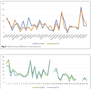
Figure 3 shows the aggregation of mutations and outliers (all aberrant KCs in each prov-ince), while Fig. 4 shows those in each sector.
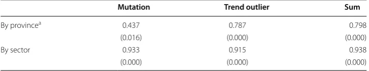
From the figures above, it is apparent that there is only a slight improvement in data quality in 2007–2012 compared with 2002–2007 when measured with aberrant KCs. However, this conclusion does not hold over all sectors and regions. Another transpar-ent conclusion is the correlation between two periods. To be precise, the Pearson cor-relation coefficients and significance tests are calculated and listed in Table 5. It turns out that all KC indicators are positively correlated when the significance level α is 0.05. In fact, expect for mutations, the correlations of all indicators are statistically significant, even when α equals 0.01.
Since no IS indicator is designed for regional evaluation, data quality in each prov-ince is given by aberrant KC indicators. Table 6 shows the five best and worst quality provinces. Some of the results, such as the poor quality of Beijing and Shanghai, may be counterintuitive, and possible explanations are offered in Sect. 4.
Fig. 3 Aberrant key coefficients in each province
3.3 IS indicators
The data quality in each sector has been evaluated and presented above. However, IS indicators still need to be calculated to assess the data quality of sectors and the whole nation’s IO data system.
3.3.1 Ratios
To identify incoherent sectors (ISs), the ratio of all provincial-level data to the real national data first has to be calculated. Take total output as an example.
This formula is compatible with all IS indicators in Table 4, except for inward/outward flow. It should apply the following formula.
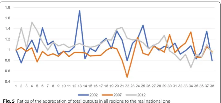
In this analysis, the data of inward/outward flows are only available in 2012. Figure 5
shows the ratios of total output calculated using the formula above.
Theoretically, all ratios should be equal or at least approximately equal to 1. How-ever, the norm is that these ratios may be a greater than or less than 1 for the following reasons.
Ratio of sector A=
Total outputs of sector A in all province National total output in sector A
Ratio of sector A=
total inward flow of sector A in all province
total outward flow of sector A in all province
Table 5 Correlation between two periods regarding aberrant key coefficients
a Numbers in parenthesis are significance level
Mutation Trend outlier Sum
By provincea 0.437 0.787 0.798
(0.016) (0.000) (0.000)
By sector 0.933 0.915 0.938
(0.000) (0.000) (0.000)
Table 6 Best and worst IO data quality regarding province in each period
a Aberrant KCs mean the ratio of aberrant KCs to all KCs, lower is better
Best data quality, 1–5 Worst data quality, 1–5
Rank Province Aberrant KCsa Rank Province aberrant KCs
Period 2002–2007 Period 2002–2007
1 Sichuan 0.000 1 Qinghai 0.253
2 Hebei 0.023 2 Hainan 0.184
2 Heilongjiang 0.023 3 Shanghai 0.149
2 Hubei 0.023 4 Beijing 0.138
2 Hunan 0.023 5 Guangdong 0.126
Period 2007–2012 Period 2007–2012
1 Hunan 0.011 1 Qinghai 0.230
1 Liaoning 0.011 2 Hainan 0.207
2 Sichuan 0.023 3 Beijing 0.149
2 Guangxi 0.023 4 Shanxi 0.126
(1) The price standard. Local producer prices are used in the regional table instead of national prices as used in the national table.
(2) Lack of data. In 2002 and 2007, Tibet did not conduct IO investigations and thus has no IO table.
(3) Statistical errors.
Despite these reasons, the differences between the aggregated data and real national data still should be slight. First, the economic scale of Tibet is small, even when com-pared to other middle and western China provinces that are less developed. Addition-ally, issues of price levels and errors are usually minor. The price levels within a country should converge according to the free market theory, and a national price level could be considered as an average. For errors, a large statistical error itself is a sign of low data quality.
3.3.2 IS indicators
In the following analysis, sectors with ratios greater than 1.2 or less than 0.8 are con-sidered incoherent sectors (ISs). In Fig. 5, the majority of total output ratios are located in this range, while there are a few ratios too large or small. However, in terms of the ratios of final demand (consumption, capital formation) and labor compensation, two features need to be stressed. First, more peculiar ratios emerge. For instance, only 19.3% of capital formation ratios lie in the range 0.8–1.2. Second, more extreme ratios emerge. Still, with respect to the capital formation ratios, some ratios are negative, and some are larger than 30. These extreme ratios indicate that the national IO data system could not maintain coherence within it, and the reliability of data should be questioned.
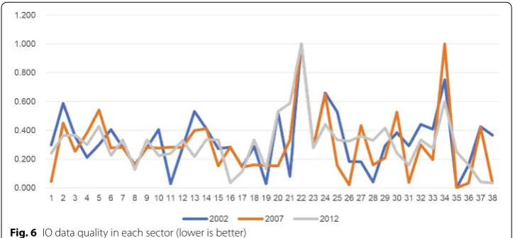
3.4 Data quality of sectors and national IO system
With all indicators calculated, the data quality of sectors and the whole system can be evaluated. First, the quality of each sector is the arithmetic average of aberrant KC indi-cators and IS indiindi-cators.1 The problem is that aberrant KC indicators are calculated in a
2-year package. To solve this, aberrant KC indicators for 2002–2007 are treated as the indicators for 2002, indicators for 2007–2012 are treated as the indicators for 2012, and the indicators for 2007 are the average of those two. Figure 6 shows the quality of indi-vidual sectors in the 3 years.
Generally, for years t0,t1,. . .,tn,tn+1 where the aberrant KCs for any next 2 years aKCij
are given, aberrant KC for a single year aKCt is defined as follows:
where i=1,. . .,n.
In Fig. 6, data qualities of scarp processing sector, gas production and supply, and R&D and technical services are the worst among all sectors in all 3 years. However, sec-tors such as agriculture and agricultural services, communication, computer and other electronic equipment, and education possess a relatively good data quality. The correla-tions between the data quality of sectors in different years are also calculated. The results (listed in Table 7) indicate that the data qualities in different years are strongly positively correlated.
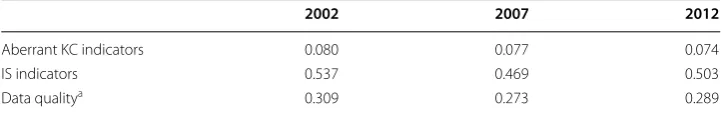
At the end of this section is the calculation of IO data quality of national IO data sys-tem, or the country as a whole. The method is the same with the calculations of sectors, and Table 8 shows the results. For overall data quality, the data quality in 2007 is only slightly better than in the other 2 years. While the fewest aberrant KC indicators occur in 2012, the IS indicators in 2007 are better to a relatively large extent. The data quality in 2002 is the worst with respect to aberrant KC indicators and IS indicators.
4 Interpretations and explanations of the result
In the results listed in Sect. 3, we easily find that the data qualities of relatively under-developed provinces (like Qinghai and Hainan) are lower than in more under-developed regions. The development extent could be the most obvious explanation that may occur.
aKC0=aKC01
aKCi= 1
2
aKCi−1,i+aKCi,i+1
aKCn+1=aKCn,n+1
Nevertheless, there are some interesting issues in conclusions, such as Beijing suffering the worst data quality, which requires interpretations and explanations. However, before the analysis, we must note there are no formal explanations that could be easily tested by empirical measures. This is due to the large quantity of data in the IO table (as we previously mentioned) and the lack of statistical data, which are necessities when testing some of the theories offered below.
First, we address the characteristics of the evaluation method itself. Limited by the features of IO data, we exploit a time-series self-referenced method that evaluates data quality by comparing the data from the same source (province, industry, or even the same cell in IO table) over different years. While this method is time and data efficient and is also easy to deploy in real-world applications, it does have weaknesses. One of them is that when structural changes occur they may not be recognized and would be considered as a sign of poor data quality, since time consistency is treated as an assump-tion and could not be violated. Thus, it is possible that the evaluaassump-tion method instead of the IO data is faulty under the following circumstances.
(1) The change in the national accounting methodology may influence the results of Guangdong in 2002–2007, since the accounting modifications concern the cessing trade. Previously, the processing trade was considered two transaction pro-cesses. One process was the importation of raw materials and intermediate prod-ucts, and the other was the exportation of finished, processed products. Therefore, it largely affected both imports and exports. However, under the current regime, only the added value of the processing trade would be measured. Similar situations hold for the construction, public management, social security and social organiza-tions sectors, whose accounting methods have been changed or at least modified. (2) Economic activity changes. Since regions such as Qinghai and Hainan have
rela-tively small regional activities compared to provinces in eastern China, the data are more likely to fluctuate. In addition, structural changes are more likely to occur due to the small quantity.
(3) Visible data improvement. Suppose the data quality in account year t is poor and
has been significantly improved in year t+1. However, since the evaluation results
depend on consistency, the improvement could not be recognized. For instance, the
Table 7 Correlations between data quality of individual sectors in different years
2002 and 2007 2002 and 2012 2007 and 2012
Correlation coefficients 0.695 0.544 0.637
Test p value (0.000) (0.000) (0.000)
Table 8 IO data quality of national IO data system
a Lower is better
2002 2007 2012
Aberrant KC indicators 0.080 0.077 0.074
IS indicators 0.537 0.469 0.503
accurate value of aij in some region is 0.010 in year t and 0.011 in year t+1. How-ever, because of some mistakes, there was a huge bias, and an inaccurate value in year t was recorded as 0.020. In the next year, they corrected the statistical methods
and the value they offered was 0.012, which is a significant improvement. However, as the data quality under the framework of this research is measured in a 2-year window, the data quality could be recognized as poor in those 2 years (instead of year t only), since there is a huge jump in the coefficient that should be stable.
According to NBS, the data quality in Beijing in 2012 may follow this trend.
(4) Major city effects. There are some specialties of major cities that should be taken into consideration. One of them is distortions due to the concentration of corpo-rate headquarters. While corporations may opecorpo-rate throughout the country, most choose to establish national headquarters in the three major cities of Beijing, Shanghai and Guangzhou. Although statistical codes require that branches in local regions should be accounted for at the regional level, it is difficult for government statistical officers to separate the activities of branches of different levels within a corporation. Therefore, at least some of the economic activities that occur in other regions are calculated in those three major cities, which could cause significant fluctuations in data consistency. For instance, even if the local branches keep their own production techniques unchanged (heterogeneous), as long as the proportions of their production to the total production change, the aggregated coefficients in major cities still may significantly fluctuate. This problem should still be consid-ered as a quality flaw. Another scenario is that developed regions are inclined to be more dynamic and less consistent because of quickly evolved technologies. Mature markets and fierce competition force businesses in developed areas to constantly upgrade their technologies and create more innovative business models. While it may seem that inconsistencies of this kind are not quality flaws, we still argue that these inconsistencies could be avoided if government statistical agencies released IO table more frequently, such as annually.
(5) False data. We regret to report that, while the data quality in Liaoning seems acceptable, the officials of the local statistical bureau admitted that they used false data to fabricate nonexistent economic booms. The most likely scenario is that they employ the same time-consistency assumption to fabricate the false data. If this is the case, it may even be useless to include more non-IO data, since the statistical agency would possibly change other data to make sure that the IO and non-IO data would not contradict each other.
to retain the accuracy and comparability of data. The best-quality province, Sichuan, retains the same official to manage its IO data.
The last explanation we offer in this section concerns the balance of the IO table. It is natural that several data are treated as balanced items in the system of the national account. In quadrant II, consumption data are considered relatively accurate since the investigation data are more detailed and frequent. In China, export data are directly recorded by customs and are recognized as even more accurate. Thus, the inward/out-ward flow in 2012 and capital formation in earlier years are treated as balanced items whose accuracy could not be assured. In other words, the data quality of these two items is not a concern of the statistical system. It is not difficult to explain why their coheren-cies are questioned by IS indicators.
5 Conclusion
In this paper, a novel framework for evaluating regional IO data has been constructed. It contains two types of indicators. Aberrant key coefficients measure accuracy and con-sistency in the time series, and incoherent sectors examine coherence. Therefore, the framework accounts for the most important standards of data quality.
The framework possesses several features. Its structure is relatively simple compared to existing data quality measuring systems. However, it covers various issues, including the data quality of regions, sectors and the national IO data system, and utilizes infor-mation from all three quadrants. Additionally, evaluations under this framework do not need additional data from other sources, which, along with its simple structure, makes the framework easy to apply.
As a trail example, China’s regional IO data are evaluated under this framework. When examined by province, both less-developed provinces (like Qinghai) and highly developed areas (like Beijing) suffer from low IO data quality. For sectors, extreme and unstable IS indicators expose a coherency problem that cannot be ignored. In terms of the national IO data system, the overall data quality is not ideal enough, and there is no significant data quality improvement between 2002 and 2012. The extent of economic development, characteristics of the evaluation framework, accounting measures and local situations are offered as explanations of the results.
Abbreviations
IO: input–output; SDDS: Special Data Dissemination Standard; GDDS: General Data Dissemination Standard; KC: key coef-ficient; aKC: aberrant key coefcoef-ficient; IS: incoherent sectors; NBS: National Bureau of Statistics of China; BEA: US Bureau of Economic Analysis.
Authors’ contributions
HZ is involved in co-construction of the evaluation framework (Sect. 2) with JX; majority of calculation of evaluation and R programming (Sect. 3); result discussion and interpretation (Sect. 4). JX raised the original idea of the paper; introduc-tion and literature review (Sect. 1); co-construction of the evaluation framework (Sect. 2) with HZ. XL is involved in data assembly and primitive calculation (Sect. 3); conclusion (Sect. 5); modification of language expression of the paper. All authors read and approved the final manuscript.
Acknowledgements
Thanks for anonymous reviewers’ generous suggestions and comments. Thanks for Huaju LI and her colleagues (National Bureau of Statistics of China) and Jianqin YUAN (State Information Center of China). They provided useful information and precious suggestions to aid the analysis in Sect. 4. The preliminary version of the paper was presented in 25th Inter-national Input–Output Association (IIOA) Annual Conference (June 2017, Atlantic City, USA) as a working paper. Thanks for conference participants’ generous suggestions. If there are some mistakes and flaws, however, authors would take full responsibilities, of course.
Competing interests
The authors declare that they have no competing interests. Availability of data and materials
All the IO data employed in this paper are available from National Bureau of Statistics of China. For the sake of conveni-ence, data can be found in Github with the web address given below. The R code for analyzing key coefficients in Sect. 3
can also be found on author’s GitHub: https://github.com/zhaohaoyangruc/IO-data-quality. Funding
Not applicable.
Appendix
See Tables 9, 10, 11, 12, 13 and 14 .
Table 9 Sector adjustment for province‑level IO table in China
a All the sectors not consistent in 3 years are moved into sector named other, which does not participate in evaluation Merge into one sector Move into sector “Other”a
General equipment, special equipment (2012) Metal products, machinery and equipment repair services (2012)
Scientific research, integrated technical services (2002) Tourism (2002)
Other social services (2002)
Water conservancy, environment and public facilities management (2007, 2012)
Table 10 Sectors after adjustment
No. Sector No. Sector
1 Agriculture and agricultural services 21 Other manufacturing 2 Coal mining products 22 Scarp processing
3 Oil and gas products 23 Production and supply of electricity and heat 4 Metal mining 24 Gas production and supply
5 Nonmetallic mining 25 Water production and supply
6 Food and tobacco 26 Construction
7 Textile 27 Wholesale and retail
8 Textile, leather and feather products 28 Transportation, storage and postal service 9 Wood products and furniture 29 Accommodation and catering
10 Paper, printing, stationery and sporting goods 30 Information transmitting, software and IT service 11 Petroleum, coking and nuclear fuel processing 31 Finance
12 Chemical products 32 Real estate
13 Nonmetallic mineral products 33 Rental and business service 14 Metal smelting and rolling processing 34 R&D and technical service
15 Metal products 35 Education
16 General and special equipment 36 Health and social work 17 Transportation equipment 37 Sports and entertainment
18 Electrical machinery and equipment 38 Public management, social security and social organizations
19 Communication, computer and other electronic
equipment 39 Others
Table 11 Aberrant KC indicators summed by province
a There are seven (2002–2007) and three (2007–2012) overlapping aberrant KCs between mutations and trend outliers, which is the reason why sums are not always equal to the real sums of mutations and trend outliers
2002–2007 2007–2012
Mutation Trend Suma Mutation Trend Sum
Beijing 1 11 12 2 11 13
Tianjin 1 8 9 4 4 8
Hebei 0 2 2 1 3 4
Shanxi 0 7 7 2 9 11
Neimenggu 3 5 8 2 4 6
Liaoning 1 2 3 0 1 1
Jilin 3 8 10 2 3 5
Heilongjiang 1 2 2 1 2 3
Shanghai 7 7 13 1 4 5
Jiangsu 0 6 6 0 2 2
Zhejiang 2 5 7 1 6 7
Anhui 0 5 5 0 3 3
Fujian 5 6 11 3 6 9
Jiangxi 1 3 4 1 6 7
Shandong 1 7 8 0 8 8
Henan 0 4 4 0 4 4
Hubei 0 2 2 1 5 6
Hunan 0 2 2 0 1 1
Guangdong 3 9 11 0 8 8
Guangxi 1 3 4 2 0 2
Hainan 5 12 16 5 14 18
Chongqing 4 6 10 0 4 4
Sichuan 0 0 0 0 2 2
Guizhou 3 3 6 2 3 5
Yunnan 1 4 5 1 4 5
Shaanxi 4 1 5 4 1 5
Gansu 1 2 3 1 4 4
Qinghai 13 11 22 4 17 20
Ningxia 3 3 6 7 4 11
Xinjiang 2 4 6 5 2 7
Table 12 Aberrant KC indicators summed by sector
a Same with Table 11, overlapping between mutations and trend outliers has been eliminated b The empty cells indicate that there are no key coefficients in that sector
Sector 2002–2007 2007–2012
Mutation Trend Suma Mutation Trend Sum
1 12 16 26 7 15 22
2 20 13 31 15 9 23
3 11 2 13 6 2 8
4 4 12 16 8 10 18
5 5 11 15 0 9 9
6 2 9 11 3 6 9
7 4 7 11 3 9 12
8 4 7 11 2 6 8
9 3 5 7 1 7 8
10 0 9 9 0 7 7
11 3 7 10 4 10 14
12 3 27 30 2 27 29
13 1 10 11 0 6 6
14 4 18 21 4 20 22
15 0 4 4 0 6 6
16 1 14 14 2 13 15
17 0 8 8 0 5 5
18 1 18 18 1 16 16
19 3 7 10 0 12 12
20 1 8 9 0 11 11
21 20 10 29 20 12 31
22b
23 5 14 17 3 11 14
24 14 5 19 14 4 17
25 0 5 5 0 6 6
26 0 2 2 0 3 3
27 5 6 10 4 7 11
28 1 11 12 0 9 9
29 3 8 10 2 8 10
30 0 1 1 0 5 5
31 0 10 10 0 8 8
32 0 4 4 0 2 2
33 0 4 4 0 3 3
34 35
36 0 2 2 0 2 2
37 2 4 6 3 2 5
38 0 2 2 0 2 2
Table 13 IO data quality in each region
a The meaning of numbers is the same with Table 6, lower is better
Province 2002–2007a 2007–2012 Province 2002–2007 2007–2012
Beijing 0.138 0.149 Henan 0.046 0.046
Tianjin 0.103 0.092 Hubei 0.023 0.069
Hebei 0.023 0.046 Hunan 0.023 0.011
Shanxi 0.080 0.126 Guangdong 0.126 0.092
Neimenggu 0.092 0.069 Guangxi 0.046 0.023
Liaoning 0.034 0.011 Hainan 0.184 0.207
Jinlin 0.115 0.057 Chongqing 0.115 0.046
Heilongjiang 0.023 0.034 Sichuan 0.000 0.023
Shanghai 0.149 0.057 Guizhou 0.069 0.057
Jiangsu 0.069 0.023 Yunnan 0.057 0.057
Zhejiang 0.080 0.080 Shaanxi 0.057 0.057
Anhui 0.057 0.034 Gansu 0.034 0.046
Fujian 0.126 0.103 Qinghai 0.253 0.230
Jiangxi 0.046 0.080 Ningxia 0.069 0.126
Publisher’s Note
Springer Nature remains neutral with regard to jurisdictional claims in published maps and institutional affiliations.
Received: 3 September 2017 Accepted: 10 November 2017 Table 14 IS indicators summed by sectors
Sector IS (2002) IS (2007) IS (2012)
1 0.500 0.000 0.400
2 1.000 0.750 0.600
3 0.500 0.333 0.600
4 0.333 0.667 0.500
5 0.500 1.000 0.800
6 0.750 0.500 0.400
7 0.500 0.500 0.600
8 0.250 0.250 0.200
9 0.500 0.500 0.600
10 0.750 0.500 0.400
11 0.000 0.500 0.400
12 0.500 0.500 0.600
13 1.000 0.750 0.400
14 0.750 0.750 0.600
15 0.500 0.250 0.600
16 0.500 0.500 0.000
17 0.250 0.250 0.200
18 0.500 0.250 0.600
19 0.000 0.250 0.200
20 1.000 0.250 1.000
21 0.000 0.500 1.000
22 1.000 1.000 1.000
23 0.500 0.500 0.500
24 1.000 1.000 0.600
25 1.000 0.250 0.600
26 0.333 0.000 0.600
27 0.250 0.750 0.600
28 0.000 0.250 0.600
29 0.500 0.333 0.750
30 0.750 1.000 0.400
31 0.500 0.000 0.250
32 0.750 0.500 0.600
33 0.750 0.333 0.500
34 0.750 1.000 0.600
35 0.000 0.000 0.250
36 0.250 0.000 0.250
37 0.750 0.750 0.000
38 0.667 0.000 0.000
References
Agafiţei M, Gras F, Kloek W, Reis F (2015) Measuring output quality for multisource statistics in official statistics: some directions. Stat J IAOS 31(2):203–211
Brackstone G (1999) Managing data quality in a statistical agency. Surv Methodol 25:139–149
Commission of the European Communities—Eurostat, International Monetary Fund, Organisation for Economic Co-operation and Development, United Nations and World Bank (1993) System of National Accounts 1993. 435–473 European Commission, International Monetary Fund, Organisation for Economic Co-operation and Development, United
Nations and World Bank (2009) System of National Accounts 2008. 507–522 Eurostat (2008) Eurostat manual of supply use and input-output tables
Eurostat (2011) European statistics code of practice. http://ec.europa.eu/eurostat/web/products-manuals-and-guide-lines/-/KS-32-11-955. Accessed 23 Feb 2017
Holz CA (2013a) Chinese statistics: classification systems and data sources. Eurasian Geographys Econo 54(5–6):532–571 Holz CA (2013b) The quality of china’s gdp statistics. A/working papers, 30(35):309–338
Huenemann RW (2001) Are china’s recent transport statistics plausible? China Econ Rev 12(4):368–372
International Monetary Fund (2013a) The general data dissemination system guide for participants and users. http:// www.imf.org/external/pubs/ft/gdds/guide/2013/gddsguide13.pdf. Accessed 23 Feb 2017
International Monetary Fund (2013b) The special data dissemination standard 2013 guide for subscribers and users.
http://dsbb.imf.org/Pages/SDDS/WhatsNew.aspx. Accessed 23 Feb 2017
James G, Witten D, Hastie T, Tibshirani R (2014) An introduction to statistical learning: with applications in R. Springer Publishing Company, Incorporated, Berlin, pp 337–372
Jin Y, Tao R (2010) The theoretical research and practice of statistical data quality in China. Stat Res 27(1):62–67 (in Chinese)
Klein LR, Özmucur S (2011) The estimation of china’s economic growth rate. J Econ Soc Meas 28(4):277–285
Liu H, Huang Y (2009) An evaluation method of statistical data quality based on the classical econometric model. Stat Res 26(3):91–96 (in Chinese)
Mehrotra A, Pääkkönen J (2011) Comparing china’s gdp statistics with coincident indicators. J Comp Econ 39(3):406–411 Miller RE, Blair PD (2009) Input-output analysis: foundations and extensions. Cambridge University Press, Cambridge, pp
69–107–349–361
OECD (2011) Quality framework for OECD statistical activities. http://www.oecd.org/std/qualityframeworkforoecdstatisti-calactivities.htm. Accessed 23 Feb 2017
Outrata E (2015) Influence of governance issues on the quality of official statistics. Stat J Iaos 31(4):523–527 Park A, Wang S (2001) China’s poverty statistics. China Econ Rev 12(4):384–398
Reis F, Gras F, Kloek W, Vâju S, Agafitei M (2015) Measuring output quality for multisource statistics in official statistics: some directions. Stat J Iaos 31(2):203–211
Sinton JE (2001) Accuracy and reliability of china’s energy statistics. China Econ Rev 12(4):373–383 United Nations (1968) A system of National Accounts. 35–51
United Nations (1999) Handbook of input-output table compilation and analysis
United Nations Department of Economic and Social Affairs Statistics Division (2003) Handbook of statistical organization, 3rd edn. https://unstats.un.org/unsd/dnss/hb/default.aspx. Accessed 23 Feb 2017
Wang H, Jin Y (2010) Statistical data quality and users’ satisfaction: designing evaluation scale and empirical study. Stat Res 27(7):9–19 (in Chinese)
Xu X (1994) The differences between the new Chinese national account system and SNA 1993 (Part II). Stat Res 11(6):24 (in Chinese)
Ye S (2011) Study on the evaluation methods of official statistical data qualityand its application. Doctoral dissertation, Hunan University. (in Chinese)
Zhang D (2003) Test methods for abnormality in statistical data. Stat Res (5):53–55 (in Chinese)