R E S E A R C H
Open Access
Mining large-scale human mobility data
for long-term crime prediction
Cristina Kadar
1*and Irena Pletikosa
1*Correspondence:[email protected] 1D-MTEC, ETH Zurich, Zurich,
Switzerland
Abstract
Traditional crime prediction models based on census data are limited, as they fail to capture the complexity and dynamics of human activity. With the rise of ubiquitous computing, there is the opportunity to improve such models with data that make for better proxies of human presence in cities. In this paper, we leverage large human mobility data to craft an extensive set of features for crime prediction, as informed by theories in criminology and urban studies. We employ averaging and boosting ensemble techniques from machine learning, to investigate their power in predicting yearly counts for different types of crimes occurring in New York City at census tract level. Our study shows that spatial and spatio-temporal features derived from Foursquare venues and checkins, subway rides, and taxi rides, improve the baseline
models relying on census and POI data. The proposed models achieve absoluteR2
metrics of up to 65% (on a geographical out-of-sample test set) and up to 89% (on a temporal out-of-sample test set). This proves that, next to the residential population of an area, the ambient population there is strongly predictive of the area’s crime levels. We deep-dive into the main crime categories, and find that the predictive gain of the human dynamics features varies across crime types: such features bring the biggest boost in case of grand larcenies, whereas assaults are already well predicted by the census features. Furthermore, we identify and discuss top predictive features for the main crime categories. These results offer valuable insights for those responsible for urban policy or law enforcement.
Keywords: Crime prediction; Urban computing; Spatio-temporal data; Human mobility; Location-based social networks; Applied machine learning
1 Introduction
Crime prediction is inherently difficult. Crime analysis has already confirmed that crimes are unequally distributed in time and space [1]. Furthermore, crime is a highly dynamic and complex phenomenon driven by the people and the environment where they meet [2], and scholars in different disciplines are still investigating various elements for predictive power. Knowing when and where crime is more likely to occur can help various actors engaged in crime reduction: urban planners to design safer cities [3] and police forces to better direct their patrols [4].
Initially, criminological studies have focused solely on socio-demographic attributes as factors correlating with victimization and have noticed that specific groups of peo-ple tend to have lifestyles that exposed them to higher risk of victimization compared to
other groups—as explained by theLifestyle Exposure Theory[5]. For instance: men, young adults, and African Americans have been found to experience higher risk of victimiza-tion in general [5]. Under the umbrella of theSocial Disorganization Theory, a series of criminological studies have explained crime as a product of the ecological attributes of the neighborhood: ethnicity, income level, and residential stability [6,7].
Cohen and Felson extended the model beyond the attributes of the underlaying popula-tions towards opportunity—according to theirRoutine Activity Theory[8] there are three elements which need to be present in time and space for a crime to occur: a motivated offender, a suitable target, and a lack of guardianship. Finally, Brantingham and Branting-ham analyzed criminogenic places in cities—places that make crime easy and profitable and are the by-products of the environments we build to support the requirements of ev-eryday life (e.g. homes, shops, offices, government buildings, parks, bus stops or sports stadia) [9]—and divided them into crime attractors and crime generators. Crime attrac-tors are places which attract criminals, because there are known opportunities in those areas. As a consequence, the probability of a crime happening in those places is higher compared to other places (e.g. night life district). In turn, crime generators are places in which crime emerges at times where large number of people are attracted to those places for reasons other than to offend (e.g. massive sports events).a
Other, more qualitative works in urban planning, have also looked at the relationship between the built environment, population and safety. Specifically, two notable works do not agree whether the density and diversity of human activity within an area are attracting crime or not. In theEyes on the Street Theory[10], Jacobs postulates that higher densities of people and buildings, pedestrian areas and a mix of activities in the neighborhood act as crime deterrents. On the other hand, Newman suggests that less built areas with more segregated activities are safer [11].
In terms of data, traditionally, quantitative models explaining crime have leveraged the socio-demographic and economical data available from the census, describing the resident population of a given neighborhood [5,7]. From a theoretical point of view, these models have relied on the initial victimization theories in criminology.
Hence, in this work, we investigate the potential of geo-tagged human dynamics data for long-term crime prediction models. We use such data to model crime attractors, crime generators and the ambient population in a neighborhood and add these factors on top of the classical factors from census that model the resident population in a neighborhood. The full models for the total number crime incidents achieve absoluteR2metrics of up to
65%when testing on neighborhoods of the same city which have not been used during the training phase of the models, and up to 89%when testing on the full data of the next year. In comparison to the census-only baselines, this translates to improvements of 30 percentage points (on a geographical out-of-sample test set) and of 7 percentage points (on a temporal out-of-sample test set). Furthermore, we look at the major crime types and show that we can achieve improvements of up to 43 percentage points and of up to 9 percentage points, respectively (for the case of grand larcenies).
2 Related work 2.1 Urban computing
Nowadays, sensing technologies and large-scale computing infrastructures produce a va-riety of big data in urban spaces: geographical data, human mobility, traffic patterns, com-munication patterns, air quality, etc. The vision of urban computing, an emerging field coined by Zheng and collaborators [14], is to unlock the power of big and heterogeneous data collected in urban spaces and apply it to solve major issues our cities face today. They identify seven application areas of urban computing: urban planning, transportation sys-tems, environmental issues, energy consumption, social applications, commercial appli-cations, and public safety and security.
A special category of this urban data consists of human dynamics data and researchers in the different application areas started to leverage it. For example, within the urban plan-ning and transportation domains, the authors in [15] attempt to infer the functions of different regions in the city of Beijing by analyzing the spatial distribution of commercial activities and GPS taxi traces, while the authors in [16] mine different urban open data sources including LBSNs in the cities of Washington, D.C. and Hangzhou for optimal bike sharing station placement. Furthermore, for commercial purposes, researchers mine LB-SNs for optimal retail store placement [17] or the London metro data for insights into the financial spending of transport users [18], and a variety of urban big data sources for pre-dicting commercial activeness [19]. Within the public safety and security sector, scholars have just recently started to investigate the potential use of social media [20], of mobile data [21], and of taxi flow data [22] for the purpose of crime inference/prediction. In a related literature stream, authors in [23] exploit POIs from different sources to build clas-sifiers of urban deprivation (a composite score of seven domains, with crime being just one of them) for neighborhoods in the UK, while authors in [13], assess the potential of subway flow data to identify areas of high urban deprivation in the city.
2.2 Crime prediction
Researchers in a wide range of fields like criminology, physics and data mining have looked at predicting crime at various scales and using different techniques. In this section we present a short overview of the existing literature.
with the population sizes of cities [24–27]. In general, these studies carry out uni-variate [26,27] or multi-variate [28] analysis of crime, i.e. crime as a function of population or of other socio-economic variables, and at a high aggregation level (that of cities). Also, at lower resolution, researchers have confirmed that crime concentrates regardless of city [29] and have found relevant allometric relations between peace disturbance and the res-ident population, as well as between property crimes and the floating population [30].
At intra-city level and using methods from statistical learning, we distinguish between two types of prediction models. The first type of models, consisting oflong-term crime prediction models, aim at modeling long-term crime level by looking at aggregated crime rates over 1 to 5 years. In terms of techniques, these models rely on classical inference models like the, sometimes geographically-weighted [22,31], Poisson [32,33] and Neg-ative Binomial [22] regressions, where the task is to predict crime levels and the perfor-mance of the model is evaluated in terms of in-sample goodness of fit. In terms of data, the traditional models in criminology make use of the classical demographic crime cor-relates, such as residential instability, ethnic heterogeneity, poverty rates, or income rates [31,32]. Moving to the data mining community, authors in [33] use census data, Open-streetMap POI data, and features of the road network to predict annual burglary levels for municipalities in Switzerland by means of regularized linear regressions tested on a one year left-out sample. Most recent work on long-term crime prediction [22] makes use of novel nodal features (Foursquare POI data next to demographic data) and edge features (geographical influence of direct neighbors or as computed by taxi flow data) to explain crime rates at community level by means of geographical linear and negative-binomial re-gressions. Similarly, authors in [34] employ spatial econometrics techniques where they compare and contrast the explanatory power of a limited set of census and Foursquare features for aggregated census tract crime levels.
started to utilize human dynamics data in short-term crime prediction models. Gerber [20] has shown that combining topics derived from the Twitter stream with the histori-cal crime density delivered by a standard KDE under a logistic regression model leads to an increase in the prediction performance of hotspots next day versus the standard KDE approach for most of the tested crime types. Combining for the first time demographic data and aggregated and anonymized human behavioral data derived from mobile data, Bogomolov and colleagues were able to obtain an accuracy of almost 70% when predicting whether a specific area in the city will be a crime hotspot or not within the next day [21].
3 Research gap and contributions
Our work lies within the category of long-term crime prediction models. Compared to previous work in this literature stream, we make following contributions:
1. in terms of data, we are the first to craft a comprehensive set of spatial and spatio-temporal features describing the dynamics of human activity in an area, as captured by the usage of social networks, public transportation, and road
transportation and use this data describing the ambient population to enhance the traditional set of features describing the resident population as modeled by the census statistics.
2. in terms of techniques, we employ latest averaging and boosting ensemble techniques from machine learning, which in comparison to the current linear models in literature, can deal with the large number of features described above. 3. in terms of evaluation, we test the models on geographical and temporal
out-of-sample test sets, to prove generalization and compare them against a weak-baseline based solely on census data and a against a strong-baseline based on census and POI data. We furthermore compare the individual predictive power of the considered data sources of human mobility: Foursquare venues/checkins, NYC subway rides, and NYC yellow and green taxis rides.
4. in terms of unit of analysis, we analyze crime at a granular level, with counts of various types of urban crime being effectively predicted at a high degree of geographic resolution, namely census tracts. We notice different degrees of predictive performance across the different crime types.
5. in terms of interpretability and unlike most studies within the urban computing community, we motivate the choice of features in criminal theory and discuss and interpret the results of the models in this context.
4 Datasets
New York City (NYC) is a city that has experienced crime across time, though the levels have dropped since the 1990s [41], some attributing the success to new policing tactics and the end of the crack epidemic [42]. Furthermore, as part of an initiative to improve the accessibility, transparency, and accountability of the city government, the NYC Open Data platformbprovides massive data in machine-readable formats on buildings, streets,
4.1 Crime data
The raw crime dataset was downloaded from the NYC Open Data platform. For anonymi-zation reasons, in case the offense has not occurred at an intersection, the New York Police Department (NYPD) projects the location of the incident to the center of the block (street segment). Furthermore, crime complaints which involve multiple offenses are classified according to the most serious offense.eNext to the total number of incidents, we
concen-trate on the following five felony types: grand larceny (which is the theft of another’s prop-erty, including money, over a certain value), robbery, burglary, felony assault, and grand larceny of motor vehicle—leaving out the murder and rape cases which have very differ-ent underlying causal mechanisms and are also reported on a higher aggregation level. We keep for analysis the data of the last 2 complete years (2014 and 2015). This yields a total number of 174,682 incidents across the five boroughs of NYC: Bronx, Brooklyn, Manhattan, Queens and Staten Island.
4.2 Census data
The census data for NYC was obtained from two separate sources, the 2010 Decennial Census, as well as the 2010–2014 and the 2011–2015 American Community Survey (ACS). In both cases, the data was fetched from the FTP sites of the US Census Bureau,fand was
filtered out to keep only the data on a census tract level.
The Decennial Census includes basic demographic figures, which are based on actual counts of persons dwelling in the US and is conducted only once every 10 years. The Sum-mary File 1, used for this study, includes items describing the population, such as gender, age, race, origin, household relationship, household type and size, family type and size, etc. In addition, housing characteristics are captured through the occupancy/vacancy status and tenure. The ACS estimates are based on yearly collected survey data over a sample of the US population. For the purposes of this study, the 5-year estimates were used, as the largest and most reliable sample, where the data is available on a census tract (and smaller) geography level. Apart from the demographics, ACS contains a rich set of social, housing and economic features, with residential stability, poverty and income being of interest for this study.
4.3 Foursquare venues data
The Foursquare dataset was collected via the Foursquare API, using the venues search and venue details endpoints. The Foursquare API has been serving both the Foursquare 8.0 and the Swarm apps since the 2014 split of the original Foursquare app. While Foursquare continues to provide a local search-and-discovery service for places near a user’s current location, Swarm lets the user share their location with friends at different precision levels (at city and neighborhood levels, or by checking-in to a specific venue).
College and University (7082), Event (84), Food (47,590), Nightlife Spot (11,140), Outdoors and Recreation (18,011), Professional and Other Places (64,055), Residence (14,632), Shop and Service (62,627), Travel and Transport (13,911). The distribution of the top categories across the venues is uneven and biased towards establishments where people go out for services, working, shopping, or dining.
4.4 Subway usage data
Subway usage data, commonly referred to as turnstile data, is released regularly by the Metropolitan Transportation Authority (MTA) and contains entries and exits audit data, generated from the Control Areas from its three main divisions: Interborough Rapid Tran-sit Company (IRT), Independent Subway System (IND) and Brooklyn-Manhattan TranTran-sit Company (BMT). While the original dataset contains data from several other associated agencies, for consistency reasons these were left out of the final dataset since the corre-sponding stations were not located within NYC, or represent train, bus or cable car sta-tions. We downloaded the turnstile data from the New York State Open Data portalgand
the MTA websitehfor the two full years of 2014 and 2015. In addition, a geocoded list of
MTA stations was also obtained from the same portal.i
To perform the preliminary data cleaning and combine the two data sources, a careful manual examination of station names was conducted. The goal was to resolve situations where the same station appeared with different names in the turnstile dataset, e.g. both ‘18 AV’ and ‘18 AVE’ where coded as ‘18 AV’, and to unify the names used in both datasets. Once the data was cleaned and merged, each station was further examined for location accuracy, by comparing and adjusting it with the corresponding station geolocation pro-vided by Google Maps. In the end, 455 distinct subway station locations were compiled. In the two years of analysis, they have experienced almost 21 million turnstile updates (the turnstile counters updated every 4 hours).
4.5 Taxi usage data
The taxi dataset was downloaded from the official website of the City of New York, specif-ically the Taxi and Limousine Commissionjand combines the 2014 and 2015 complete
records of both yellow and green taxi trips. These are the two types of services permitted to pick up passengers via street hails, thus offering a great footprint of human activity. Furthermore, yellow cabs are concentrated around Manhattan and the two main airports (JFK International Airport and LaGuardia Airport), while green cabs are allowed above the 110th Street in Manhattan and in the outer-boroughs of New York City. With the two datasets joined, we obtain a good coverage of the whole city. The trip records include fields capturing pick-up and drop-off timestamps and locations, next to other meta-data like driver-reported passenger counts and trip distances. We have processed in total over 340 millions taxi drives for this work.
5 Model specification 5.1 Unit of analysis
show the explicit effect of both the resident population (as recorded by census) and of the ambient population (as recorded by the different proxies) on the raw counts. As a tech-nical remark: we look in the following at points situated in the area of each census track, buffered by 50 feet (which is half the width of the main Manhattan avenues), to account for potential precision inaccuracies in the different spatial data types and to integrate the crime locations that lie on the bordering streets. The same applies for venues, subway, and pickup/drop-off locations.
Census tracts provide a stable set of geographic units for the presentation of statistical data and generally have a population size between 1200 and 8000 people, with an optimum size of 4000 people.kIn the case of NYC they span a few blocks and offer a natural unit for
crime analysis at a detailed level. NYC has a total of 2167 official census tracts. A few of these consist only of water or shoreline areas, which have not been experiencing any crime incidents in either of the analysis years. Furthermore, some NYC census tracts consist fully of military posts or jail facilities (like e.g. Fort Hamilton and Rikers Island) which exhibit different crime reporting schemes, next to restricted human presence. We remove these census tracts, and remain with a final ofN= 2154 census tracts. Please note we still include many census tract with no resident population, like parks or airports, as these still experience crime, and now we have the possibility to model it by means of the ambient population measured by the alternative data sources. For visualization purposes, Fig.1 depicts the 2015 aggregated crime counts per census tract, together with some example features computed at census tract level. All maps in this paper have been generated using the open source software QGIS.l
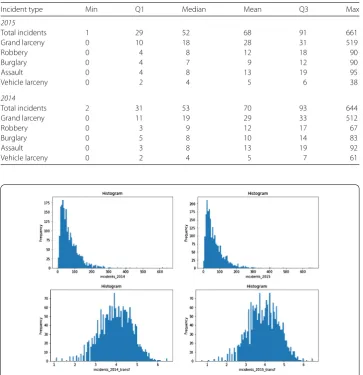
Table1presents the descriptive statistics of crime counts of all types, while Fig.2is de-picting the histograms of the total incidents counts per census tract. We can observe that the distribution of the data is positively skewed with many observations having low count
Table 1 Descriptive statistics of the crime data: counts per census tract for each year
Incident type Min Q1 Median Mean Q3 Max
2015
Total incidents 1 29 52 68 91 661
Grand larceny 0 10 18 28 31 519
Robbery 0 4 8 12 18 90
Burglary 0 4 7 9 12 90
Assault 0 4 8 13 19 95
Vehicle larceny 0 2 4 5 6 38
2014
Total incidents 2 31 53 70 93 644
Grand larceny 0 11 19 29 33 512
Robbery 0 3 9 12 17 67
Burglary 0 5 8 10 14 83
Assault 0 3 8 13 19 92
Vehicle larceny 0 2 4 5 7 61
Figure 2Histogram of the original and log-transformed total incidents per census track: 2014 (left) and 2015 (right)
values. The various crime types expose also similar power law distributions, so for the pre-diction task below, we log-transform the dependent variable to correct for the positively skewed distribution, and use this as our dependent variabley.
5.2 Prediction features
the data for feature generation per unit of analysis, as described in the remainder of this section.
5.2.1 Census features
To account for the fact that the units of analysis are heterogeneous, we include the census tract’sarea(in square miles) andtotal populationas controls in the regression. We then proceed with a standard set of factors deemed in past criminological studies as signifi-cantly influential of crime and have been used also in related work in data mining, like [22].
We start by operationalizing the concepts of theLifestyle Exposure TheoryandSocial Disorganization Theory. We start with indicators of population at risk and of concentrated disadvantage [5–7]:fraction of male population,fraction of black population,fraction of hispanic population,fraction of population under the poverty level. As violence has been associated with residential instability of neighborhoods [7,43], we compute thefraction of vacant households, thefraction of rented householdsfrom the occupied ones, and the fraction of stable population(individuals who moved in prior to 2010).
Furthermore, population diversity has been shown to play a role in the crime phe-nomenon [10, 32, 43] so we computed several diversity indexes based on the socio-demographic and economical information: aracial ethnic diversity index, anage index, and anincome diversity index. The racial ethnic index is defined by the plurality of multi-ple ethnic and racial groups within a certain area and is computed based on five exhaustive and mutually exclusive aggregates (non-Hispanic whites, non-Hispanic blacks, Hispanics of any race, Asians, and others—Native Americans, members of other races, and multi-racial persons) [44]. The age index measures the variance in ages of the residents across four main age groups (under 18, 18–34, 35–64, and over 65 years), and the income in-dex measures the variance in household income across three main income levels (low, medium, and high-income households) [45].
5.2.2 Spatial features
This category of features describes the characteristics of a neighborhood, as captured by the spatial distribution of the Foursquare venues and subway stations within its perimeter. In general, the venues can be seen ascrime attractors—particular places to which offenders are attracted because of the known opportunities for particular types of crimes [9].
Thenumber of venues of each categorymeasures the venues counts within a census tract and it is a static popularity metric of that area. Thefractions of venues of each category capture the specifics of the life within a census tract, and it is an empirical metric for the functional decomposition of that particular area in the city. Thevenues diversity index is then a single measurement capturing the diversity of this decomposition. Inspired by [17], we use the entropy measurement from information theory [46] as a diversity metric. Intuitively, the entropy quantifies the uncertainty in predicting the category of a venue that is taken at random from the area. The final formula models the normalized Shannon diversity index (also called the Shannon equitability index [47]), which is the Shannon diversity index divided by the maximum diversity. For a given census tractti, we denote the
count of included venues of categorycwithVc(ti) and the total number of included venues
employ smoothing by adding the constant 1 to the numerator and denominator to prevent zero divisions):
–
c∈C
1 +Vc(ti)
1 +V(ti) ×
ln1 +Vc(ti)
1 +V(ti)
ln|C|.
The higher the index, the more heterogeneous the area is in terms of types of places, and following that, in terms of functions and activities of the neighborhood, whereas a least entropic area would indicate an area with a dominant function. For example, a census tract dominated by venues from the College and University category, would indicate a part of the city where people primarily study and would have a low diversity index.
Motivated by the work in [23], we generate a metric called theoffering advantagewhich denotes to what extent a particular neighborhood offers more venues of a particular cat-egory in comparison to the average neighborhood. Intuitively, the presence of one venue of an unpopular category, is more informative in profiling a neighborhood than the pres-ence of one venue from a well-spread category. The offering advantage of categorycin each census tracttiof the totalNcensus tracts in NYC, is computed with the following
formula:
1 +Vc(ti)
1 +V(ti) ×
total_venues
N
i=1Vc(ti)
,
wheretotal_venuesis the number of total venues in NYC with an assigned category. Finally, based on the MTA dataset, we compute thetotal number of subway stations within each census tract, to reflect whether the area is subject to high-volume population transit from other parts of the city.
5.2.3 Spatio-temporal features
In this section, we derive metrics of human activity in that area. We compute, analog to the census data, metrics of density and diversity—but, while the census features exploit information about the reported residential population, the human dynamics features are computed based on the ambient population, as measured by their usage of public venues and transportation. Overall, the features in this categories describe possiblecrime genera-tors. Crime generators produce crime by creating particular times and places that provide appropriate concentrations of people and other targets [9]. These features can also be con-nected to theRoutine Activity Theory, as they model the activity nodes where motivated offenders meet vulnerable targets.
Thenumber of checkins per categorymeasure the popularity of the area. The empirically observed Foursquare checkins can be regarded as a more accurate measure of human activity than the traditional population density statistics from the census.
We further exploit Foursquare usage in each census tract, by looking at the popular hours of the venues (those times of the week where the venues experience most activity— checkins, reviews, etc.) and compute thenumber of venues that are popular in a typical morning, afternoon, evening or night—split by weekdays and weekendsin each. These fea-tures give valuable information about the temporal break-down of human activity in the area.
contexts in which the population engages. For instance, an area with many checkins in the Residence category would correspond to a residential neighborhood, which is very differ-ent to an differ-entertainmdiffer-ent district, that would in turn be characterized by a high number of checkins in the Food, Nightlife Spot, and Shop and Service categories. We proceed by computing thecheckins diversity index, as an index of the distribution of human activity within the census tract. It can be seen, that the venues and checkins diversity indexes are the best operationalization of Jacobs’ and Newman’s concept of mixed land use.
Inspired by recent work on digital neighborhoods [48], we computelocal quotientsof (digital) social activity within an area. LetC(ti) denote the total number of checkins and
P(ti) the total population count within a census tract. We then compute the concentrations
of checkins relative to the number of businesses and to the reference census population:
1 +C(ti)
total_checkins×
total_venues 1 +V(ti)
,
1 +C(ti)
total_checkins×
total_population 1 +P(ti)
,
wheretotal_checkinsdenotes the number of total checkins in NYC, andtotal_population the total census population of NYC. Neighborhoods with local quotients1 can be re-garded as (digital) hot spots, while neighborhoods with local quotients1 can be re-garded as (digital) deserts.
It can be observed, that the offering advantage and the local quotient metrics are both refined measures of therelative intensity of human activityin an area as opposed to the whole city (one being based on the static distribution of the venues, and the other on the more dynamic distribution of the checkins).
To make use of the temporal dimension of the turnstile subway data, we aggregate it toweekly averages of the number of individuals entering and exiting the subway stations— split into Mon–Fri and Sat–Sun intervals. We also compute asubway rides diversity index, by considering these four different categories: subway entries/exists in week/weekend.
Finally, we exploit the taxi ride data and computedweekly averages of the number of pas-sengers being picked up or dropped off in the census tracts—split into Mon–Fri and Sat–Sun intervals. Complementary to the popular hours of the venues, and the subway features, these features should give an additional indication of the average in- and out-flows of the population traveling to and from the area. Finally, we compute ataxi rides diversity index, by considering the numbers of pick-up/drop-off rides within the neighborhood.
Across all three feature categories, we end up with a total of 89 features. For exemplifi-cation purposes, Fig.1depicts a selection of the 2015 features computed at census tract level. Spearman correlation tests and linear regressions have revealed significant corre-lations between many of the features and the differentyvariables—see Additional file1 (section Descriptive Statistics). We decided to keep them all for the following step, where the chosen machine learning algorithms, due to their internal structure, will be able to deal with higher number of (potentially correlated) features and rank them according to their predictive power.
exploit a high number of features but use domain knowledge to generate them. This ap-proach is prevalent in the urban computing and data science literature, used for instance: to identify optimal retail store placement [17], to quantify the relationship between urban form and socio-economic indexes [49], or to understand economic behavior in the city [50].
6 Results
6.1 Model evaluation
We train three different tree-based machine learning models: a Random Forest regressor [51], an Extra-Tree (Extremely Randomized Tree) regressor [52], and a Gradient-Boosting regressor [53]—all known in the literature for their ability to yield competitive prediction quality in high-dimensional heterogeneous feature spaces. Due to their non-parametric nature, they make no assumption about the data and can work with many, collinear fea-tures, while also requiring little preparation of the data [54]. On the other hand, linear models assume that the explaining variables are non-collinear, which is not the case in our data-rich setup. Furthermore, a linear model has proved to yield poor performance on our datasets and is not reported.
Random forests are very popular in practice, as they are easy to use, robust, and yield good performance. An entire set of decision trees are grown at training time, and their mean prediction is output at testing time, thus lowering the variance of the individual learners. The Extra-Trees add a third level of randomization in comparison to the ran-dom forests, in that the split tests at each node of the decision trees are ranran-dom, next to the chosen sub-sets of samples and features. In practice, they yield sometimes better performance thanks to the introduced smoothing effect, and also remove computational burdens linked to the determination of optimal cut-points in random forests. While these first two models are averaging models and build their constituent decision trees in parallel, Gradient-Boosting builds the model in a stage-wise fashion. It constructs additive regres-sion models by sequentially fitting a simple base learner on the current pseudo-residuals. Boosted trees have been shown to be the best performing models across a variety of tasks, at least in the pre-deep-learning era [55].
In addition, all these tree-based ensemble methods can be exploited to infer the rela-tive importance of the input variables (based on the order in which they appear in the constituent decision trees) and to rank them accordingly [54].
Internally, the regressors always optimize the mean squared error (MSE) total number of log-transformed incidentsy, and we report two metrics:MSE, as well as the coefficient of determination (R2). TheMSEmetric is given by1
n
n
i=1(yi–yˆi)2, with lower scores being
preferred. TheR2metric measures the percentage of variance in the dependent variable
that the model at hand explains: 1 – n
i=1(yi–yˆi)2
n
i=1(yi–y¯i)2, whereyi are the true values,yˆi are the predicted values, andy¯iis the mean of the sample. Best possible score is 1.00 and it can
be negative (because the model can be arbitrarily worse). A constant model that always predicts the expected value ofy, disregarding the input features, would get a score of 0.00. It primarily helps us to compare models between the different feature configurations, but it can also be used to compare the performance on the different incident types, as it is independent of the sample range.
baseline consisting only of the socio-demographic and economical factors derived from the census sources. The second model is a strong baseline consisting additionally of the numbers of Foursquare venues/POIs per category. This model specification is designed to reproduce the nodal features from [22]. We ought to note that the venues dataset might be slightly different from a standard dataset of POIs inferred for example from Open-StreetMap or Google Maps, as the Foursquare venues set is biased towards establish-ments where people spend time, and map already better to the concept of crime attractors then standard POIs. Hence, we expect that venues counts would outperform standard POI counts as features in crime prediction models. The third model is making use of all human dynamics features inferred from the mobility data sources, while the forth model is a full specifications, exploiting the complete set of features.
Furthermore, in Additional file1, we create three further model specifications, where each makes use, additionally to the standard census features, of the full feature set of a given data source: Foursquare, subway rides, and yellow/green taxi rides. This enables a direct comparison of the ubiquitous data sources in terms of their predictive power for the crime domain—in case in practice a model selection decision should be required.
For each machine learning model, incident type, and features subset combination, we estimate the performance of the algorithms on new unseen data. To asses their geographi-calout-of-sample generalization, we do the followingmodel evaluationexperiment using nested cross-validation. In a nested cross-validation, two cross-validation loops are per-formed: one outer loop to measure the prediction performance of the estimator and one inner loop to choose the best hyper-parameters of the estimator. We implement this ap-proach with 5 outer loops formodel assessment(i.e. setting the size of the test set to 20%), and 2 inner loops formodel selection(i.e. setting the size of the training and validation sets to 40%, respectively). Table2presents the final averageMSEandR2scores and standard
deviations of the models on the left-out test subsets. The resulting scores are therefore unbiased estimates of the prediction score on new geographical samples. We also pro-vide atemporalevaluation of the approaches, by training a model on the complete 2014 data (with 5-fold CV for hyper-parameter tuning, i.e.model selection) and testing it on the unseen 2015 data formodel assessment.
Across all experiments, the hyper-parameters optimized in the validation phase of the Random Forest and Extra-Trees are the number of trees in the ensemble (values rang-ing from 50 to 400) and the maximal depth (values rangrang-ing from one third, to one half, to the full set of features). The first parameter controls the model complexity, while the second controls the level of pruning of the trees, in other words performing regulariza-tion to avoid overfitting. For Gradient Boosting, we perform a grid search over the num-ber of trees (values ranging from 100 to 400), the maximal depth (values ranging from 1 to 4), and also the learning rate (values ranging from 0.01 to 0.2). The models were imple-mented in Python v2.7, with the help of the scikit-learnnand pandasolibraries. Additional file1(section Model Assessment) presents validation and learning curves of the employed models. The validation curves show that we have properly chosen the parameter ranges for hyper-parameter tuning. Also, the learning curves show that, in our case, the models keep improving with more data, so we should use all available samples.
6.1.1 Geographical evaluation
Ta b le 2 Geog raphical out -of-sample results of the reg re ssors using d iff er ent subsets of the featur e s: fo r e ach ye ar ,r epeat e dly trained on 80% of the census trac ts ,and test e d o n 20% of the census trac ts C e nsus C e nsus + P OI Human D ynamics C ensus + Human D ynamics MSE R 2 MSE R 2 MSE R 2 MSE R 2
2015 Total
incidents R andom Fo re st 0.58 ± 0.11 0.33 ± 0.19 0.46 ± 0.05 0.58 ± 0.07 0.55 ± 0.07 0.38 ± 0.20 0.44 ± 0.03 0.62 ± 0.03 Ex tra-Tr ee 0.57 ± 0.10 0.35 ± 0.16 0.45 ± 0.04 0.60 ± 0.06 0.55 ± 0.03 0.40 ± 0.07 0.43 ± 0.03 0.63 ± 0.03 Gradient Boosting 0.57 ± 0.10 0.35 ± 0.16 0.44 ± 0.04 0.61 ± 0.06 0.57 ± 0.06 0.36 ± 0.08 0.42 ± 0.03 0.65 ± 0.03 Gr and lar ce nies R andom Fo re st 0.72 ± 0.17 0.14 ± 0.18 0.53 ± 0.05 0.52 ± 0.08 0.53 ± 0.05 0.52 ± 0.10 0.50 ± 0.04 0.57 ± 0.06 Ex tra-Tr ee 0.70 ± 0.15 0.18 ± 0.12 0.52 ± 0.05 0.53 ± 0.08 0.53 ± 0.05 0.52 ± 0.08 0.50 ± 0.04 0.57 ± 0.06 Gradient Boosting 0.71 ± 0.15 0.16 ± 0.13 0.53 ± 0.05 0.52 ± 0.08 0.53 ± 0.05 0.52 ± 0.08 0.49 ± 0.03 0.59 ± 0.07
Robberies Random
Fo re st 0.70 ± 0.05 0.36 ± 0.11 0.65 ± 0.05 0.46 ± 0.10 0.77 ± 0.06 0.23 ± 0.13 0.62 ± 0.04 0.50 ± 0.08 Ex tra-Tr ee 0.69 ± 0.06 0.38 ± 0.12 0.64 ± 0.04 0.47 ± 0.07 0.77 ± 0.04 0.23 ± 0.10 0.62 ± 0.04 0.49 ± 0.08 Gradient Boosting 0.68 ± 0.05 0.40 ± 0.11 0.63 ± 0.05 0.48 ± 0.09 0.77 ± 0.03 0.22 ± 0.09 0.62 ± 0.04 0.49 ± 0.08 Bur g laries R andom Fo re st 0.60 ± 0.04 0.19 ± 0.03 0.55 ± 0.03 0.31 ± 0.05 0.62 ± 0.04 0.13 ± 0.12 0.56 ± 0.03 0.30 ± 0.06 Ex tra-Tr ee 0.59 ± 0.04 0.21 ± 0.06 0.56 ± 0.03 0.31 ± 0.04 0.61 ± 0.03 0.16 ± 0.08 0.55 ± 0.04 0.31 ± 0.05 Gradient Boosting 0.57 ± 0.03 0.27 ± 0.04 0.55 ± 0.03 0.32 ± 0.04 0.63 ± 0.02 0.11 ± 0.06 0.56 ± 0.03 0.29 ± 0.04 A
ssaults Random
Ta b le 2 ( C ontinued ) C e nsus C e nsus + P OI Human D ynamics C ensus + Human D ynamics MSE R 2 MSE R 2 MSE R 2 MSE R 2
2014 Total
incidents R andom Fo re st 0.58 ± 0.10 0.29 ± 0.18 0.45 ± 0.06 0.57 ± 0.09 0.56 ± 0.06 0.35 ± 0.10 0.44 ± 0.05 0.59 ± 0.06 Ex tra-Tr ee 0.58 ± 0.10 0.30 ± 0.17 0.45 ± 0.05 0.58 ± 0.09 0.57 ± 0.06 0.32 ± 0.09 0.44 ± 0.05 0.59 ± 0.06 Gradient Boosting 0.58 ± 0.08 0.29 ± 0.14 0.45 ± 0.05 0.58 ± 0.06 0.56 ± 0.08 0.34 ± 0.14 0.45 ± 0.06 0.59 ± 0.08 Gr and lar ce nies R andom Fo re st 0.70 ± 0.15 0.13 ± 0.17 0.52 ± 0.07 0.52 ± 0.09 0.53 ± 0.06 0.49 ± 0.08 0.50 ± 0.06 0.56 ± 0.07 Ex tra-Tr ee 0.69 ± 0.14 0.17 ± 0.13 0.51 ± 0.07 0.53 ± 0.08 0.54 ± 0.06 0.49 ± 0.06 0.50 ± 0.07 0.56 ± 0.06 Gradient Boosting 0.72 ± 0.16 0.09 ± 0.17 0.52 ± 0.08 0.52 ± 0.08 0.53 ± 0.07 0.49 ± 0.05 0.49 ± 0.06 0.57 ± 0.05
Robberies Random
Fo re st 0.70 ± 0.04 0.35 ± 0.11 0.65 ± 0.06 0.44 ± 0.12 0.80 ± 0.05 0.16 ± 0.16 0.64 ± 0.05 0.47 ± 0.10 Ex tra-Tr ee 0.70 ± 0.04 0.36 ± 0.11 0.64 ± 0.06 0.47 ± 0.10 0.81 ± 0.05 0.13 ± 0.18 0.63 ± 0.05 0.48 ± 0.10 Gradient Boosting 0.69 ± 0.05 0.37 ± 0.12 0.64 ± 0.06 0.46 ± 0.11 0.81 ± 0.08 0.12 ± 0.25 0.62 ± 0.04 0.50 ± 0.08 Bur g laries R andom Fo re st 0.64 ± 0.04 0.19 ± 0.02 0.59 ± 0.03 0.30 ± 0.05 0.63 ± 0.05 0.21 ± 0.08 0.58 ± 0.03 0.31 ± 0.05 Ex tra-Tr ee 0.63 ± 0.03 0.20 ± 0.03 0.58 ± 0.02 0.32 ± 0.03 0.64 ± 0.05 0.18 ± 0.07 0.58 ± 0.03 0.32 ± 0.05 Gradient Boosting 0.61 ± 0.03 0.27 ± 0.01 0.58 ± 0.03 0.33 ± 0.02 0.64 ± 0.06 0.18 ± 0.09 0.58 ± 0.04 0.32 ± 0.05 A
ssaults Random
and census + POI baselines for all incident types, with the exception of burglaries and as-saults, where the models already saturate at the hard baseline of census + POI. For the total number of incidents we achieve a competitiveR2score of 65%, followed by the grand larcenies, robberies, and assaults categories with scores from 50% to 59%, while for bur-glaries and especially for vehicle larcenies the scores are lower. This can be explained by the fact that the latter categories of crime are not driven by the population characteristics, but by the characteristics of the target: house and car, respectively. As we do not include attributes of the built environment and of the stollen goods in the models, it was expected that these specific two categories would generally perform worse in comparison to the other categories.
For the total number of incidents, the best model on the full data set achieves scores of 65%, which is 30 percentage points better than the best model in the weak-baseline and 4 percentage points better than the hard-baseline. But the highest improvement that we observe in comparison to the census-only baseline is in the case of grand larcenies: roughly 41 and 7 percentage points, respectively. This crime category includes different kinds of thefts, including pickpocketing. It was therefore expected that data describing the popularity of an area would be most informative, yet the improvement is spectacular. The weak baseline performs best for the assaults category. This category groups offenses that involve inflicting injury upon others, and it is already well explained by the collected socio-demographic and economical attributes of the neighborhood.
Furthermore, for the case of total incidents and grand larcenies, we observe that mod-els based solely on attributes of the ambient population outperform the modmod-els based on the classical demographic features—and, in the case of grand larcenies, even reach per-formance levels comparable with those of the census + POI baseline. Finally, comparing the datasource-specific models (provided in Additional file1—section Additional Model Specifications), we conclude that the census + FS consistently outperforms the census + subway and the census + taxi models—with the exception of the vehicle larcenies crime category, which performs poorly across the board. Comparing the additional predictive power of the subway vs taxi rides, we notice a significant advantage of the taxi usage data in case of the grand larcenies category.
Inspecting the results for the 2014 geographical prediction, we deduce very similar in-sights: the full models for the total incidents, grand larcenies and the robberies categories perform best, with their absolute achievedMSE/R2scores being slightly bigger/lower than
on the 2015 data.
6.1.2 Temporal evaluation
Table 3 Temporal out-of-sample results of the regressors using different subsets of the features: trained on 2014 and tested on 2015
Census Census + POI Human
Dynamics
Census + Human Dynamics
MSE R2 MSE R2 MSE R2 MSE R2
Total incidents
Random Forest 0.11 0.82 0.07 0.88 0.09 0.84 0.07 0.88
Extra-Tree 0.11 0.82 0.07 0.89 0.08 0.87 0.07 0.89
Gradient Boosting 0.22 0.64 0.09 0.85 0.12 0.80 0.08 0.87
Grand larcenies
Random Forest 0.19 0.73 0.14 0.81 0.14 0.81 0.13 0.82
Extra-Tree 0.21 0.71 0.14 0.81 0.14 0.80 0.14 0.80
Gradient Boosting 0.28 0.61 0.17 0.77 0.16 0.78 0.15 0.79
Robberies
Random Forest 0.27 0.71 0.24 0.75 0.28 0.70 0.23 0.75
Extra-Tree 0.26 0.72 0.23 0.75 0.27 0.70 0.27 0.71
Gradient Boosting 0.38 0.59 0.29 0.69 0.32 0.66 0.28 0.70
Burglaries
Random Forest 0.25 0.47 0.24 0.50 0.25 0.47 0.24 0.49
Extra-Tree 0.25 0.47 0.24 0.50 0.33 0.32 0.32 0.34
Gradient Boosting 0.30 0.38 0.25 0.47 0.27 0.42 0.23 0.51
Assaults
Random Forest 0.24 0.75 0.22 0.77 0.28 0.72 0.22 0.77
Extra-Tree 0.24 0.76 0.22 0.78 0.28 0.71 0.27 0.73
Gradient Boosting 0.34 0.65 0.29 0.71 0.46 0.53 0.24 0.76
Vehicle larcenies
Random Forest 0.31 0.31 0.29 0.34 0.31 0.31 0.30 0.34
Extra-Tree 0.33 0.27 0.29 0.36 0.37 0.16 0.38 0.15
Gradient Boosting 0.32 0.28 0.31 0.30 0.34 0.23 0.30 0.33
FS-derived features (census + POI, census + FS, and the full model) achieve the highest absolute scores.
6.2 Model interpretation
We now turn tomodel interpretation, where the focus will be (1) on examining the im-portance and the contribution of the individual features defined in Sect.5.2and (2) on understanding where in the city do the ambient population features improve the baseline models.
6.2.1 Feature importance
This exercise will return those features that proved to be most discriminative for geo-graphical crime prediction task. By examining them, we will be able to understand what type of factors are most relevant for the predictive algorithms, and also identify those criminological theories that have informed the best features. It is important to stress the fact that, these techniques would not allow us to infer any causal relationships between the features and the crime counts. The identified factors are most discriminative in the context of the used model, but they not necessarily best explain crime levels.
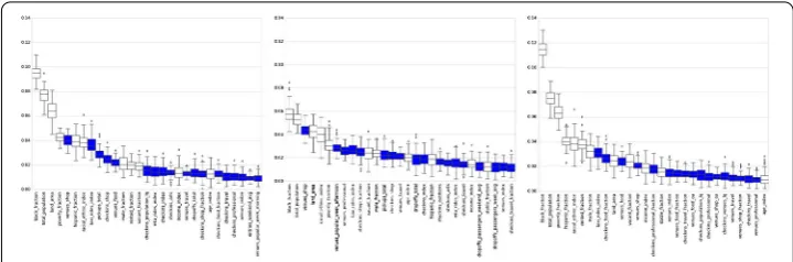
Figure 3Variable importance plots (top one third of the variables) reported by the Gradient Boosting Models (full specification). From left to right: 2015 total incidents, 2015 grand larcenies, and 2015 assaults
samples (80% of the data) and provide a box-plot ranked by the median importance of the outputs returned by the different samples. Figure3visualizes the top one third variables in these rankings: in white features inferred from the census, in blue features inferred from human mobility data.
The traditional census features score indeed high across all three crime categories and across all algorithms. Specifically, we observe their very high contribution in the assaults model. As already hinted in the previous section, this type of violent crime remains best predicted by the attributes of the residential population in an area.
Also the spatial features from Foursquare have significant contributions across all mod-els. The shopping venues contribute most in the grand larcenies category, followed by professional and travel venues. On the other hand, the food establishments, followed by the shopping establishments have a significant contribution in the assaults models.
In terms of spatio-temporal features from Foursquare, we see importance assigned to many features derived from checkins data, like checkins in food and shops and checkins diversity index. We also see that the number of afternoon popular venues during the week receives a high weight for the grand larcenies category.
In terms of human dynamics features inferred from the taxi data, we notice especially high loadings for the diversity index of the taxi drives and the total number of pickups and for the in the larcenies and total incidents categories. The human dynamics features inferred from the subway data have in general a lower predictive contribution, with the diversity index ahaving the relative higher scores in this features subgroup and making it into the top features for total incidents and grand larcenies.
6.2.2 Partial dependence plots
The above feature importance rankings only tell uswhichfeatures are predictive of crime, but nothowthey contribute to the models. There are several approaches on how to achieve that. One approach is to plot partial dependency plots of the gradient boosting learners, another approach is to fit simple decision trees on the top discriminative features of the full models and extract prediction rules.
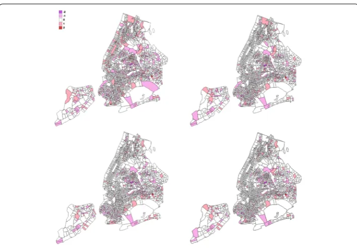
Figure 5Absolute error of predicted vs actual values for the 2015 larcenies counts per census tract. From left to right, and top to down: census (weak baseline), census + POI (strong baseline), FS + subway + taxi (human dynamics), and census + FS + subway + taxi (full model)
with higher population numbers, higher poverty, and higher percentage of rented houses tend to have higher crime levels. Also, neighborhoods in NYC with a higher percentage of minorities tend to have higher crime levels, with a stronger effect noticed in the assaults category. On the other hand, we also notice that highly diverse neighborhoods might be slightly safer. The POIs features exhibit strong marginal effects: especially census tracts with shopping establishments tend to experience more grand larcenies, and census tracts with food establishments tend to experience more assaults. From the spatio-temporal fea-tures, taxi drives diversity exhibits a positive relationship with the crime level across all three categories. Finally, neighborhoods with more popular venues during working day afternoons are associated with higher number of larcenies.
6.2.3 Geographical improvement
Finally, to understand the additive predictive power of the human dynamics features in the case of the temporal prediction, we do a deeper analysis of the residuals. Figure5presents the absolute error (computed asyi–yˆi, rounded to integer precision) of the best
mod-els (Random Forest regressors) on the different model specifications for the 2015 grand larcenies crime category. There are 1652 (out of 2154) census tracts with an absolute er-ror between –0.5 and 0.5 in the census weak-baseline. This number increases to 1838 in the census + POI strong-baseline, and to 1850 in the full model specification. Notably, the human dynamics specification achieves a competitive high number of 1808 census tracts with low errors. Additional file1depicts the absolute errors achieved by the remaining model specifications.
models. Looking at the function of the neighborhoods, these models bring improvements for parks (e.g. Central Park or Prospect Park), entertainment areas (e.g. around the NY Aquarium or the College Point Multiplex Cinemas) or the JFK airport. Between the hard-baseline incorporating only FS venues information and the model incorporating also FS check-in information, we notice improvements for instance in the Brooklyn promenade recreational areas or in the shopping areas south-east of College Point.
7 Conclusions 7.1 Implications
In this paper, long term crime prediction has been investigated at a fine-grained level, with yearly crime data being analyzed at census track level and across several crime categories. In constructing the prediction features, we exploited census data, Foursquare venues data, subway usage data, and taxi usage data by operationalizing different concepts from crim-inological and urban theories. Our work has both theoretical and practical implications.
First, we have identified new crime predictors derived from massive ubiquitous data sources and so extended the empirical literature in urban computing and computational social science. Our results show that, enriching the traditional census features describing the characteristics of the residential population with spatial and spatio-temporal features describing the activities of the ambient population, substantially improves the quality of the prediction models. Factors describing criminogenic places (crime attractors and crime generators) [9] prove therefore essential for competitive crime prediction models. The highest improvement they bring has been observed in predicting crime in busy public parts of the city: recreational area and parks, shopping areas, entertainment areas, and airports. The human dynamics features improve the baseline models for the total number of incidents, for grand larcenies, and for robberies. In terms of the analyzed sources of timestamped geo-referenced human activity data, LBSNs achieve the highest predictive power. Enhancing the models with subway or with taxi data yields similar results, with the exception of the grand larcenies category, where the taxi features exhibit a higher predic-tive ability.
In general, the best performing novel features for all crime incidents have been: the total number of shopping/eating/travel venues and checkins as proxy for the general popularity of that area, the number of popular venues in a normal afternoon as proxy for the temporal break-down of human activity in the area, the total number of taxi pick-ups as proxy for the population outer flow to more remote areas, and the taxi drives index as proxy for the entropy of the human movement in the area. Many of these top features can be mapped as crime attractors or crime generators and have been informed by the theories that the place and time where the offenders and victims meet are strong crime predictions [8,9]. While the mixed land use concept theorized by Jacobs and Newman have not been found as particularly discriminative for crime prediction in comparison to the other features, Jacob’s metrics of raw human density and activity have been found to strongly improve the models. Furthermore, specific novel predictors emerge for specific crime types.
From the census features, the metrics of concentrated disadvantage have scored highest across all crime types, which is aligned with the findings within the frameworks of the Social Disorganization Theory [6,7].
recreational areas. So far, crime prevention through environmental design (CPTED) [56] has concentrated mostly on the attributes of the built environment (e.g. lightning, visibil-ity, access and height of buildings) and less so on the human activity that will be generated within the new created space. A derived product can also be used by individuals (either locals or tourists) to assess the incidents risk when traveling, going out or going shopping to new areas that they are not familiar with. Furthermore, an extension of the presented prediction models could be operationally deployed by local police agencies for short term risk assessment and effective deployment of patrol resources. Forces on the ground could better target specific types of crimes expected in a small geographical area. Current soft-ware solutions like PredPolponly work effectively for burglaries and rely mostly on recent
crime (near-repeat victimization) and less on attributes of the environment or of the am-bient population. Our findings therefore expand the scope to street crimes and utilize further information on the time and place of potential crimes.
7.2 Discussion
Our results add to existing body of empirical literature. Compared to [57], we go beyond correlation analysis between human dynamics features and crime counts, and explore a highly multi-variate non-linear prediction setup. While our diversity and ratio metrics do not match one-to-one, similar metrics to the ones used in this work make it also to our top most discriminative features, e.g. the age diversity index. Yet, we are careful to interpret the results as supporting or opposing Jacobs’/Newman’s theories, as the relationships be-tween the population density and diversity and crime are non-causal and non-linear in our case. Similarly to [22], we generally find that features derived from the venues consistently improve the basis models based solely on census data. In comparison to their work, we go beyond simple POI counts and derive second-order features from Foursquare informed by works in criminology and urban computing, and also additionally exploit sources of mo-bility patterns: subway and taxi drives. While they employed standard regression models, we employed non-parametric machine learning models, which boosted the performance. Also, similar to [21], we demonstrate the potential of human dynamics features for the crime domain. In comparison to their work, we leverage Foursquare, subway, and taxi data instead of telecommunication data, which is arguably easier to access for research and poses less ethical questions. We also run a more comprehensive analysis leveraging: (1) more extensive datasets in terms of temporal coverage of the collected data (weeks ver-sus years) and (2) several machine learning techniques for a more difficult prediction task (regression versus binary classification). Finally, compared to all of these previous works, we are the only ones to take deeper dives into the different crime types and do careful model interpretation.
used for prediction, but not for inferring a causal effect between the features and the de-pendent variable.
We should acknowledge the geographical (more urban areas) [58] and social bias (younger, more educated, wealthier users) [12] of Foursquare in general, though the choice of NYC (as the city with most activity on Foursquare) and of the complete aggregated in-formation on venues level (as opposed to incomplete extracts of checkins on users level which are common in literature) are good mitigation approaches. Quantifying such bi-ases would become relevant once comparing different locations [59], but are for now out of scope for this study.
Also, we ought to acknowledge the reporting bias present in the crime data itself. Bias in police records can be attributed to: (1) levels of community trust in police, in case of self-reported crimes, and (2) patrolling focus on certain ethnic groups and neighborhoods, in case of police-reported crimes. Even if we do not have the ambition of solving the perpet-uation of racial biases in police work, we should note that this can introduce dangerous biases [60]. Training models on biased historical data and having police focus on certain communities, will lead to even more arrests of minorities, but will not lead to solving the crime problem. The solution is not trivial, as it lies at the heart of the interaction between the police and the communities. At higher levels of aggregation, “ground truth” crime data could be estimated from crime victimization surveys and demographically representative synthetic populations [60].
Finally, to be aligned with previous work in criminology [6] and to be able to benchmark against prior work on crime prediction [22], we have used the race of the inhabitants when crafting several of the census features for the prediction problem. A potential mitigation would be to show how well the models do without taking race into consideration, espe-cially if planned to be used operationally. In this work, we have already shown that, for certain types of crime, models using only human mobility data can out-perform the mod-els based only on the census data. We believe this to be a significant contribution and an important step towards more fairness in crime prediction.
7.3 Future work
For future work and to make more general claims about the predictive power of such fac-tors for long-term crime prediction globally, we plan to apply the same methodology on data from other major cities around the globe. Furthermore, the models can be enhanced by exploiting further ubiquitous data sources describing the pulse of our cities, like ad-ditional social media signals, 311 calls, and IoT devices. Especially for some specific type of crimes, like burglaries and vehicles thefts, incorporating spatial features describing the built environment (houses, streets, land use, etc.), has the potential to improve the mod-els significantly. Finally, introducing temporal crime correlates (weather data, near-repeat patterns, entertainment events, etc.) has support in criminology and the potential to im-prove our prediction models towards short-term prediction.
Additional material
Acknowledgements
We would like to thank Raquel Rosés Brüngger for her valuable insights into criminology.
Funding
Not applicable.
Abbreviations
ACS, American Community Survey; BMT, Brooklyn-Manhattan Transit Company; ET, Extra-Trees; GB, Gradient Boosting; IND, Independent Subway System; IRT, Interborough Rapid Transit Company; LBSN, Location-Based Social Networks; MTA, Metropolitan Transportation Authority; MSE, Mean Squared Error; NYC, New York City; NYPD, New York Police
Department; RF, Random Forests.
Availability of data and materials
All data (crime dependent variable and processed features) can be requested directly from the authors.
Competing interests
The authors declare that they have no competing interests.
Authors’ contributions
CK collected part of the data, designed the experiments, carried out the analysis, prepared the figures, and wrote the manuscript. IP collected part of the data and discussed with CK the initial design of the study. Both authors read and approved the final manuscript.
Authors’ information
CK is a doctoral researcher at the Department of Management, Technology, and Economics (D-MTEC) of the Swiss Federal Institute of Technology in Zurich (ETH Zurich) and has been awarded the IBM PhD Fellowship for her academic achievements. She holds a MSc with Honors from the Elite Graduate Program in Software Engineering, a joint initiative of three Bavarian universities: Technical University of Munich, Ludwig Maximilian University of Munich, and University of Augsburg. IP was a post-doctoral researcher at the Department of Management, Technology, and Economics (D-MTEC) of the Swiss Federal Institute of Technology in Zurich (ETH Zurich). She holds a PhD in Management Science from the same institution, and a MSc in Electrical Engineering and Computer Science from Ss. Cyril and Methodius University Skopje.
Endnotes
a We have limited our survey of theories in criminology to the main theories that look at victims and offenders and
their routine activities, and are relevant for this study. Indeed, there are also other factors that influence criminal behavior, such the attributes of the built environment. For instance, Wilson and Kelling proposed in theirBroken Windows Theory[61] that degraded urban environments (such as broken windows, graffiti, excessive litter) enhance criminal activities in the area.
b https://nycopendata.socrata.com/
c http://www.foursquare.com/
d http://www.4sqstat.com/
e https://data.cityofnewyork.us/Public-Safety/NYPD-7-Major-Felony-Incidents/hyij-8hr7
f http://www.census.gov/
g https://data.ny.gov/en/browse?q=turnstile
h http://web.mta.info/developers/turnstile.html
i https://data.ny.gov/Transportation/NYC-Transit-Subway-Entrance-And-Exit-Data/i9wp-a4ja
j http://www.nyc.gov/html/tlc/html/about/trip_record_data.shtml
k https://www.census.gov/geo/reference/gtc/gtc_ct.html
l http://www.qgis.org/en/site
m http://postgis.net/
n http://scikit-learn.org/stable/
o http://pandas.pydata.org/
p http://www.predpol.com
Publisher’s Note
Springer Nature remains neutral with regard to jurisdictional claims in published maps and institutional affiliations.
Received: 2 February 2018 Accepted: 29 June 2018
References
1. Brantingham PJ, Brantingham P (1993) Environment, routine, and situation: toward a pattern theory of crime. In: Clarke RVC, Felson M (eds) Routine activity and rational choice: advances in criminal theory. Taylor & Francis, New York
2. Miethe TD, Meier RF (1994) Crime and its social context: toward an integrated theory of offenders, victims, and situations. Book News, Inc., Portland
3. Clarke RV (2009) The theory of crime prevention through environmental design. Police Manag Stud Q 3(3):344–356 4. Braga AA (2005) Hot spots policing and crime prevention: a systematic review of randomized controlled trials. J Exp
5. Hindelang MJ, Biderman AD, Gottfredson MR, Garofalo J (1982) Victims of personal crime: an empirical foundation for a theory of personal victimization. Ballinger Publishing Co
6. Pratt TC, Cullen FT (2005) Assessing macro-level predictors and theories of crime: a meta-analysis. Crime Justice 32:373–450.
7. Sampson RJ, Rauenbush SW, Earls F (1997) Neighborhoods and violent crime: a multilevel study of collective efficacy. Science 277:918–924
8. Cohen LE, Felson M (1979) Social change and crime rate trends: a routine activity approach. Am Sociol Rev 44:588–608
9. Brantingham PP, Brantingham PP (1995) Criminality of place. Eur J Crim Policy Res 3:5–26 10. Jacobs J (1961) The death and life of great American cities. Vintage, New York
11. Newman O (1973) Defensible space: crime prevention through urban design. Ekistics 36:325–332
12. Cranshaw J, Hong JI, Sadeh N (2012) The livehoods project : utilizing social media to understand the dynamics of a city. In: ICWSM’12
13. Smith C, Quercia D, Capra L (2013) Finger on the pulse: identifying deprivation using transit flow analysis. In: CSCW’13 14. Zheng Y, Capra L, Wolfson O, Yang H (2014) Urban computing: concepts, methodologies, and applications. ACM
Trans Intell Syst Technol 5:38
15. Yuan J, Zheng Y, Xie X (2012) Discovering regions of different functions in a city using human mobility and POIs. In: KDD’12
16. Chen L, Zhang D, Pan G, Ma X, Yang D, Kushlev K, Zhang W, Li S (2015) Bike sharing station placement leveraging heterogeneous urban open data. In: UbiComp’15
17. Karamshuk D, Noulas A, Scellato S, Nicosia V, Mascolo C (2013) Geo-spotting: mining online location-based services for optimal retail store placement. In: KDD’13
18. Lathia N, Capra L (2011) Mining mobility data to minimise travellers’ spending on public transport. In: KDD’11 19. Yang S, Wang M, Wang W, Sun Y, Gao J, Zhang W, Zhang J (2017) Predicting commercial activeness over urban big
data. Proc ACM Interact Mob Wearable Ubiquitous Technol 1:1–20
20. Gerber MS (2014) Predicting crime using Twitter and kernel density estimation. Decis Support Syst 61:115–125 21. Bogomolov A, Lepri B, Staiano J, Oliver N, Pianesi F, Pentland A (2014) Once upon a crime: towards crime prediction
from demographics and mobile data. In: ICMI’14
22. Wang H, Kifer D, Graif C, Li Z (2016) Crime rate inference with big data. In: KDD’16
23. Venerandi A, Quattrone G, Capra L, Quercia D, Saez-Trumper D (2015) Measuring urban deprivation from user generated content. In: CSCW’15
24. Bettencourt LMA, Lobo J, Helbing D, Kühnert C, West GB (2007) Growth, innovation, scaling, and the pace of life in cities. Proc Natl Acad Sci USA 104(17):7301–7306.
25. Bettencourt LMA, Lobo J, Strumsky D, West GB (2010) Urban scaling and its deviations: revealing the structure of wealth, innovation and crime across cities. PLoS ONE 5(11):e1354.
26. Alves LGA, Ribeiro HV, Lenzi EK, Mendes RS (2013) Distance to the scaling law: a useful approach for unveiling relationships between crime and urban metrics. PLoS ONE 8(8):e69580.
27. Alves LGA, Mendes RS, Lenzi EK, Ribeiro HV, Rozenblat C (2015) Scale-adjusted metrics for predicting the evolution of urban indicators and quantifying the performance of cities. PLoS ONE 10(9):e013486.
28. Alves LGA, Ribeiro HV, Rodrigues FA (2017) Crime prediction through urban metrics and statistical learning. arXiv:1712.03834
29. Oliveira M, Bastos-Filho C, Menezes R (2017) The scaling of crime concentration in cities. PLoS ONE 12(8):e0183110. 30. Caminha C, Furtado V, Pequeno THC, Ponte C, Melo HPM, Oliveira EA, Andrade JS (2017) Human mobility in large
cities as a proxy for crime. PLoS ONE 12(2):e0171609.
31. Taylor RB, Ratcliffe JH, Perenzin A (2015) Can we predict long-term community crime problems? The estimation of ecological continuity to model risk heterogeneity. J Res Crime Delinq 52:635–657
32. Osgood DW (2000) Poisson-based regression analysis of aggregate crime rates. J Quant Criminol 16:21–43 33. Kadar C, Zanni G, Vogels T, Cvijikj IP (2015) Towards a burglary risk profiler using demographic and spatial factors. In:
WISE’15
34. Kadar C, Brüngger RR, Pletikosa I (2017) Measuring ambient population from location-based social networks to describe urban crime. In: SocInfo’17
35. Eck J, Chainey S, Cameron J, Wilson R (2005) Mapping crime: understanding hotspots. Technical report, U.S. Department of Justice
36. Short MB, D’Orsogna MB, Pasqour VB, Tita GB, Brantingham PJ, Bertozzi AL, Chayes LB (2008) A statistical model of criminal behavior. Math Models Methods Appl Sci 18(Suppl.):1249–1267.
37. Mohler GO, Short MB, Brantingham PJ, Schoenberg FP, Tita GE (2011) Self-exciting point process modeling of crime. J Am Stat Assoc 106:100–108
38. D’Orsogna MR, Perc M (2015) Statistical physics of crime: a review. Phys Life Rev 12:1–21.
39. Wang X, Brown DE (2011) The spatio-temporal generalized additive model for criminal incidents. In: ISI’11 40. Wang X, Brown DE (2012) The spatio-temporal modeling for criminal incidents. Secur Inform 1:2
41. Langan PA, Durose MR (2003) The remarkable drop in crime in New York city. In: International conference on crime 42. Blumstein A, Wallman J (2000) The rise and decline of hard drugs, drug markets, and violence in inner-city New York.
In: The crime drop in America. Cambridge University Press, Cambridge, pp 164–206
43. Graif C, Sampson RJ (2009) Spatial heterogeneity in the effects of immigration and diversity on neighborhood homicide rates. Homicide Stud 13:242–260
44. Lee BA, Iceland J, Sharp G (2012) Racial and ethnic diversity goes local: charting change in American communities over three decades key findings. Technical report, Brown University
45. Lima A, Melnik M (2010) Boston: measuring diversity in a changing city. Technical report, Boston Redevelopment Authority