O R I G I N A L A R T I C L E
Open Access
Sparse-view tomography via displacement
function interpolation
Gengsheng L. Zeng
1,2Abstract
Sparse-view tomography has many applications such as in low-dose computed tomography (CT). Using under-sampled data, a perfect image is not expected. The goal of this paper is to obtain a tomographic image that is better than the naïve filtered backprojection (FBP) reconstruction that uses linear interpolation to complete the measurements. This paper proposes a method to estimate the un-measured projections by displacement function interpolation. Displacement function estimation is a non-linear procedure and the linear interpolation is performed on the displacement function (instead of, on the sinogram itself). As a result, the estimated measurements are not the linear transformation of the measured data. The proposed method is compared with the linear interpolation methods, and the proposed method shows superior performance.
Keywords:Limited data imaging, Tomography, Estimation
Introduction
Low-dose computed tomography (CT) can be achieved by using either lower current or fewer projection views. Sparse-view tomography thus can find applications in low-dose CT [1]. Another application is in fast magnetic resonant imaging (MRI) when radial k-space sampling scheme is utilized [2]. In sparse-view tomography, mea-surements are under-sampled, which usually result in severe aliasing artifacts as streaking lines in the
recon-structed images. The phrase “sparse-view” means that
the number of views in data acquisition is significantly smaller than the value that is met by Shannon’s sampling theorem, which requires [3].
Np≈Dmin ð1Þ
where Np is the number of views over 180° andDminis the minimum number of detector bins to cover the object at one view. Many systematic studies lead to more efficient sampling criteria [4–8], where more compli-cated two-dimensional interpolations are discussed.
According to compressed sensing theory, sparse-view tomography may still be possible if some image domain
constraints are used to compensate for the missing data [9–15]. However, this paper focuses on analytic filtered backprojection (FBP) reconstruction. Iterative recon-struction methods and machine learning methods are beyond the scope of this paper.
Sometimes the unmeasured views can be
approxi-mately estimated by interpolation methods [16–19].
Recently, machine learning methods are popular and successful in sparse-view data estimation [20–22].
In this paper, we argue that interpolation with linear convolution approaches simply introduce slightly rotated
images to the main image. By the “main” image, we
imply the image that is reconstructed by only the mea-sured sparse data. The results of machine learning methods depend on the training sets; therefore, the results may not be applicable to all applications. Here we propose a nonlinear method to estimate unmeasured projections by using displacement functions, which will be discussed in Section II. The linear interpolation method assumes that the unmeasured value is the aver-age of its neighbors. On the other hand, the deformation method assumes that the unmeasured value has the same value as one of its neighbor’s value. The deform-ation method is nonlinear and is able to avoid or reduce the rotational interpolation artifacts. Comparison simu-lations will be presented in Section III, and Section IV concludes the paper.
© The Author(s). 2019Open AccessThis article is distributed under the terms of the Creative Commons Attribution 4.0 International License (http://creativecommons.org/licenses/by/4.0/), which permits unrestricted use, distribution, and reproduction in any medium, provided you give appropriate credit to the original author(s) and the source, provide a link to the Creative Commons license, and indicate if changes were made.
Correspondence:[email protected]
1Department of Engineering, Utah Valley University, 800 West University
Parkway, Orem, UT 84058, USA
2Department of Radiology and Imaging Sciences, University of Utah, 729
Methods
The rotation effect of the linear interpolation method
As a simple example to illustrate the main motivation, this paper first considers a naïve linear interpolation approach that doubles the number of views in tomog-raphy. Let the sinogram be p(n, m), where pis the line integral of the object,nis the detector bin index and m is the view angle index. In this example, whenmis odd, thep(n,m) is measured. Whenmis even, thep(n, m) is not measured and needs to be estimated. A simple linear interpolation scheme to estimate p(n, 2m) from p(n, 2
m-1) andp(n, 2m+ 1) is
p nð ;2mÞ ¼0:5½p nð ;2m−1Þ þp nð ;2mþ1Þ ð2Þ
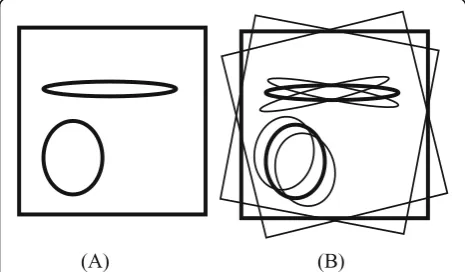
The ultimate effect of this interpolation scheme is exaggeratingly illustrated in Fig.1as an outline drawing, where the under-sampling streaking artifacts are not
shown. Figure 1a shows the main image reconstructed
from the original sinogram, while Fig. 1b shows the
image reconstructed from the interpolated sinogram using (2). It is interesting to observe from Fig. 1b that the reconstructed image from the interpolated sinogram is a combination of three components: the main recon-struction using the original under-sampled sinogram (with a weighting factor of 1), a rotated version of the
main reconstruction by Δγ (with a weighting factor of
0.5), and a rotated version of the main reconstruction by
-Δγ (with a weighting factor of 0.5). Here 2Δγ is the
angular gap between two adjacent views in the original under-sampled sinogram.
An intuitive way to understand this phenomenon is to consider a different example that copies the available measurements at view 2m+ 1 to view 2m, i.e., p(n, 2m) =p(n, 2m+ 1). Using the extended sinogram, the re-constructed image will be the summation of two images: one is the original image and the other is a rotated version of the original image.
In general, sinogram interpolation via convolution yields an image that is a combination of the main struction and some rotated versions of the main recon-struction. Similar phenomena are expected for other sinogram estimation methods that based on linear interpolation.
These two simple examples imply that in order to significantly improve the sinogram estimation, we must use some sort of nonlinearity. The idea of non-rigid deformation may be borrowed, altered, and applied to
our sinogram estimation [23–25]. Another non-linear
way is to use sine wave approximation [17]. This paper proposes a displacement function interpolation method.
Use the deformation function for non-linear interpolation
The main idea of our algorithm is illustrated below. A pair of measured sinogram views is provided: p(n, m1) andp(n, m2), wherenis the index along the radial direc-tion andm1and m2are two angular indices. The goal is to estimatep(n, m) withmbetweenm1andm2.
The first step of the proposed method is to find a displacement functionu(n) to connectp(n, m1) andp(n,
m2) so that
p nð ;m2Þ≈p nð þu nð Þ;m1Þ ð3Þ
It is desired to find a displacement function u(n) by minimizing the objective function
Fn¼ ½p nð ;m2Þ−pðnþn uð Þ;m12 ð4Þ
for eachn. Sincenis an index, we could requiren(u) to be an integer.
It is fairly flexible how to define an objective function
F. As another example, we can add the sign function of
the finite difference to the objective function as.
F¼½p nð ;m2Þ−p nð þu nð Þ;m1Þ2
þλ½signðp nð ;m2Þ−p nð −1;m2ÞÞ−signðp nð þu nð Þ;m1Þ −p nð þu nð Þ−1;m1ÞÞ2
ð5Þ
where λ is a pre-set parameter to balance the
weight-ing between constraints in the objective function F. We set λ= 0.01 in our implementation of (5). The purpose of the sign function is to encourage that the slopes of the deformed function p(n+u(n),m1) and the target functionp(n,m2) have the same sign.
If we restrictu(n) to be integers in [−N,N] withN be-ing a pre-set positive integer, it is efficient to evaluate the objection F with all possibleu(n) values in [−N, N] and use a “min” function to determine the optimal dis-placement function u(n). Here, “min” is a built-in func-tion in Matlab® to find the minimum value in an array. The motivation of using the“min”function instead of an Fig. 1Outline diagrams for images reconstructed (a) from the
original under-sampled sinogram and (b) from interpolated sinogram
iterative algorithm (such as the gradient decent algo-rithm) is to make the algorithm more efficient. The
“min” function method only evaluates the deformed
function 2N+ 1 times, while an iterative method evalu-ates the deformed function at least equal to the number of iterations, which is much greater than 2N+ 1.
After the displacement function u(n) is found, in the
second step, the un-measured sinogram p(n, m) with m
between m1and m2can be readily obtained by linearly
interpolating the displacement function u(n). For
ex-ample, if m2 – m1=M+ 1, we can estimate M views
betweenm1andm2as
p nð ;mÞ≈p nþm−m1
M u nð Þ;m1
ð6Þ
form=m1, m1+ 1,…,m2−1. We must point out that in (6)n+u(n) × (m−m1)/Mis most likely not an integer. Let
n1¼ nþ
m−m1
M u nð Þ
j k
ð7Þ
and
α¼nþm−m1
M u nð Þ−n1 ð8Þ
where⌊x⌋is the largest integer that is not greater than
x. Then (6) cab be expressed as
p nð ;mÞ≈ð1−αÞp nð 1;m1Þ þαp nð 1þ1;m1Þ ð9Þ
form=m1,m1+ 1,…,m2−1.
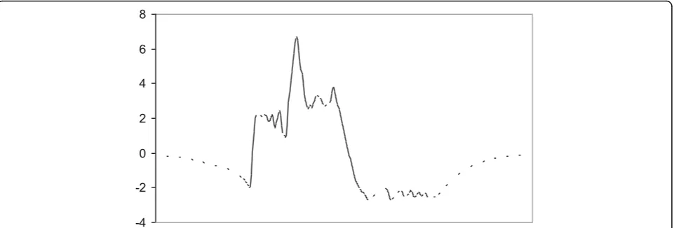
An illustrative example for the proposed estimation
procedure is shown in Fig. 2, where we have two
sino-gram measurements: p(n, 2m+ 1), as a broken curve,
and p(n, 2m-1), as a solid curve. Our proposed algo-rithm discussed above gives a displacement function,
u(n), as shown in Fig.3, so that
Fig. 2Projections at two adjacent view angles from the original under-sampled sinogram. One is shown as a broken curve. The other is shown as a solid curve
p nð ;2mþ1Þ≈p nð þu nð Þ;2m−1Þ ð10Þ
The unmeasuredp(n,2m) is then estimated as
p nð ;2mÞ≈p nð þ0:5u nð Þ;2m−1Þ ð11Þ
Since 0.5u(n) may not be an integer, linear
interpolation is required as suggested by (9). Similarly,
p(n, 2m) can be estimated by the measurement at view 2
m+ 1 with a displacement function v(n), or by the
combined measurements at both view 2m-1 and view 2
m+ 1 as
p nð ;2mÞ≈p nð þ0:5u nð Þ;2m−1Þ þp nð þ0:5v nð Þ;2mþ1Þ 2
ð12Þ
Computer simulations and patient study
This proposed sinogram extension method was applied to two computer simulation cases and one real patient case. In the computer simulations, the image size was 256 × 256, and the detector size was 367. In this paper, the word “sinogram” is used in a general sense, and the “sinogram” can be parallel projections and can be fan-beam projections or in other geometries.
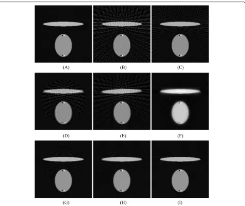
In computer simulations, the original under-sampled sinogram was generated analytically without noise. We Fig. 4FBP reconstructions reconstructed bya360 measured views,b60 measured views,c120 measured views,d360 views created from 60 views by sinc function interpolation,e360 views created from 60 views by linear interpolation,f360 views created from 60 views by proposed deformation method,g360 views created from 120 views by sinc function interpolation,h360 views created from 120 views by linear interpolation, andi360 views created from 120 views by proposed deformation method
can better observe the image distortion in noiseless stud-ies. In the first computer simulation study, the original measured number of views was 60 over 360°. After sino-gram extension, the number of views was increased to 180 over 360°. In the second computer simulation study, the original measured number of views was 120 over
360°. After sinogram extension, the number of views was increased to 360 over 360°. The absolute error image be-tween the estimated sinogram and the true sinogram was calculated and reported in the next section.
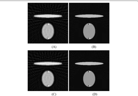
In the patient study, the sinogram data was obtained by a CT scan using 500 mAs. The detector was curved, Fig. 5Iterative Landweber reconstructions with 1000 iterations reconstructed bya60 measured views,b120 measured views. Iterative
Landweber reconstructions with 2000 iterations reconstructed byc60 measured views,d120 measured views
and the imaging geometry was cone-beam. The central slice of the cone-beam data was used as the fan-beam data. The data set had 896 detector bins at one view and 1200 views over 360°.
In this paper, an under-sampled data set was a subset of the original data set by using only 400 fan-beam views over 360°. After sinogram extension with displacement interpolation, there were 1200 views over 360°.
Sinogram estimation results using two-adjacent-view linear interpolation was also obtained and reported in the next section.
The root mean square error (RMSE) between the re-construction and the true image was calculated for all reconstruction images. The RMSE is defined as
RMSE¼ ffiffiffiffiffiffiffiffiffiffiffiffiffiffiffiffiffiffiffiffiffiffiffiffiffiffiffiffiffi 1 n Xn i¼1
Ri−Ti
ð Þ2
s
ð13Þ
where Ri is the reconstruction pixel value and Ti is the true image value. For the patient study, the true image was not available and is substituted by the reconstruc-tion with the full data set using 1200 views.
For the comparison purposes, an iterative Landweber
algorithm was also used in image reconstruction [26].
The iterative Landweber algorithm can be expressed as
Xðkþ1Þ¼Xð Þk þαATAXð Þk−P ð14Þ
where A is the projection matrix,AT is the backprojec-tion matrix, αis a relaxation parameter (or step size), P is the projection sinogram re-formatted in the vector form, andX(k)is the reconstructed image at the kth iter-ation re-formatted in the vector form. The parameter α in this paper is chosen as 0.01.
Results
Rotation displacement artifacts due to sinogram linear interpolation
Linear interpolation between sinogram views is equiva-lent to linear combination of the images from the ori-ginal sparse-view reconstruction and rotated versions of the sparse-view reconstruction. These effects are illus-trated by an exaggerated sketch in Fig.1. The rotational artifacts become more severe at locations away from the center-of-rotation in the image. The observation of these artifacts motivated the investigation of a nonlinear sino-gram interpolation method.
Using function deformation for sinogram interpolation
Figure 2 shows two curves p(n, m1) and p(n, m2), one being a solid curve and the other being a broken curve. These two curves represent two sinogram measurements at view indicesm1andm2. A displacement functionu(n) was estimate according to (3) so that the deformed ver-sion of one function approximately equal the other func-tion (p(n,m2)≈p(n+u(n),m1)) . The displacement function is shown in Fig.3.
Using the displacement function u(n) for sinogram
interpolation was realized as follows. A missing view at the angle exactly between the two measured views can be estimated by replacingu(n) by 0.5 ×u(n).
Computer simulations
Figure 4 shows the results from the computer
simula-tions with the FBP reconstruction algorithm. In this set, measurements from 360 views over 360° are considered Table 1Computer simulation sinogram estimation errors
Initial data set
Methods Maximal absolute errors in the expanded sinogram
Sum of absolute errors in the expanded sinogram 60 views Linear interpolation 0.8635 6419.9 Sinc interpolation 0.1698 390.2537
Proposed 0.1254 268.4655
120 views Linear interpolation 0.1015 108.0924 Sinc interpolation 0.0898 142.4612
Proposed 0.0776 97.0789
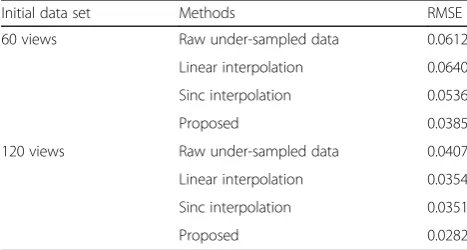
Table 2Computer simulation FBP reconstruction errors in RMSE
Initial data set Methods RMSE
60 views Raw under-sampled data 0.0612
Linear interpolation 0.0640
Sinc interpolation 0.0536
Proposed 0.0385
120 views Raw under-sampled data 0.0407
Linear interpolation 0.0354
Sinc interpolation 0.0351
Proposed 0.0282
Table 3Computer simulation iterative reconstruction errors in RMSE
Sinogram views Number of iterations RMSE
60 views 1000 0.0364
2000 0.0362
120 views 1000 0.0681
2000 0.0680
as a full sinogram, and measurements from 60 views over 360° and 120 views over 360° are considered as
under-sampled. Figure4a, b and c show the FBP
recon-struction results from the full and under-sampled sinograms, respectively. Fig.4d, e and f show the results with linear convolution sinogram interpolation methods: sinc function interpolation and linear interpolation, as well as the proposed deformation method, respectively; the initial data set had 60 views. Figure4g, h and i show the results with linear convolution sinogram interpolation
methods: sinc function interpolation and linear
interpolation, as well as the proposed deformation method, respectively; the initial data set had 120 views. The linear interpolation method is equivalent to the tri-angle function convolution method. Figure4f and i show the results of the proposed non-linear method.
There are two pairs of small black-and-white dots in the phantom. The pair at the bottom is blurred more than the pair at the center be the estimation algorithms. We also observe that for the linear methods there is a circular region and the background noise texture is different within and outside this region.
The iterative Lanweber algorithm was used to struct the image using under-sampled data. The recon-struction results are shown in Fig.5for the data set with 60 views and the data set with 120 views, respectively.
The estimated sinograms and the true sinogram are compared in terms of the absolute value of the differ-ence in Fig.6for the estimation methods used in Fig.4. A summary of the absolute errors in the estimated
sino-grams is listed in Table 1. A summary of the RMSE in
the FBP reconstructions is listed in Table2. Table3lists Fig. 7(Gold standard) FBP reconstruction using full sinogram with angular gap = 0.3° (1200 views over 360°). Left image display window: [min, max]. Right image display window: [−400, 400] HU
the RMSE in the iterative reconstructions. The recon-struction errors for the iterative algorithm reconstruc-tions depend on the iteration number, which is chosen by the user according to the applications. A lower iter-ation number gives a blurrier image, but less streaking artifacts.
There are two types artifacts: the under-sampling streaking texture in the uniform areas and the blurry artifacts due to sinogram interpolation. The blurring artifacts can be easily detected by the pair of black-and-white dots at the bottom of the image. All methods perform poorly for the data set that has only 60 views.
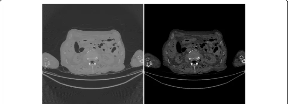
The study results using the patient CT data are shown in Figs. 7, 8, 9, 10, 11, 12. In this study set, measure-ments from 1200 views over 360° are considered as a full
sinogram, and measurements from 400 views over 360° are considered as an under-sampled sinogram. The detector had 896 bins for each view. The reconstructed image size was 800 × 800. Figure7shows the FBP reconstruction with this 1200-view full data set and is considered to be the gold standard for other reconstructions to compare with.
Figure8shows the FBP reconstruction with 400 views.
This image contains lots of streaking artifacts due to angular aliasing. For patient images, all images are displayed twice using two different display windows: [min, max] and [−400, 400] Hounsfield units (HU).
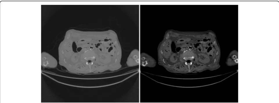
Figure 9 shows the FBP reconstruction result from
linear interpolation method. Severe rotation artifacts are observed in the image. The most severe rotation artifacts are observed at the outer regions inside the patient. Fig. 9FBP reconstruction using linearly interpolated sinogram with old angular gap = 0.9° and new angular gap = 0.3° (1200 views over 360°). Some rotation artifacts are observed. Left image display window: [min, max]. Right image display window: [−400, 400] HU
Figure 10 shows the result of proposed method that uses a non-rigid deformation technique. The rotation ar-tifacts are no longer present. However, this image is not perfect. Compared with the gold standard shown in Fig.7, some shadow artifacts are observed along the high contrast boundaries, and the spatial resolution is some-what degraded.
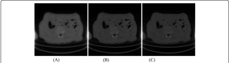
In order to appreciate the improvements of the pro-posed method, a small rectangular sub region at the right part of the original image is cut out and is displayed in a larger format in Fig.11for images in Figs.7,8,9,10.
Figure 12 show three iterative reconstruction images
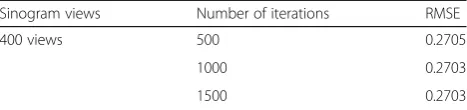
obtained with 500, 1000, and 1500 iterations, respect-ively. The number of views was 400 over 360°. The image resolution improves as the number of iteration in-creases. At the 1500th iteration, the reconstructed image is still blurry. RMSEs for the iterative reconstrction re-sults are presented in Table4for the patient study.
Conclusions
Few-view tomography in CT is an open problem. This paper made an observation that linear convolution-based sinogram interpolation methods may produce
rotational artifacts. To overcome this problem, this paper suggests a nonlinear method to estimate the un-measured views. In this proposed method, two adjacent views in the original under-sampled sinogram are used to estimate the missing views between them. A displace-ment function is estimated by a non-iterative method. A fraction of the displacement function is used to estimate the missing views between the original measurements. One advantage of the proposed method is that the resultant FBP reconstruction using the estimated sinogram does not have the rotation artifacts. Our estimated sinogram is more accurate than the sinogram estimated by linear convolution-based methods, which is demonstrated by the absolution errors as shown in Tables1,2and3.
In our patient study, there are 400 views over 360° and there are 896 bins on the detector. The number of view angles is extremely small, about 1/4.5 of the value
required by the Shannon’s sampling theorem. The
proposed algorithm produces fewer artifacts than the linear interpolation method as demonstrated in Fig.11.
The iterative Lanweber algorithm is also used for the under-sampled data image reconstruction. However, it requires a large number of iterations to produce high Fig. 11Zoom-in images of a sub rectangular region at the right of each image in Figs.8,9,10,11fromatod. Left images display window: [min, max]. Right images display window: [−400, 400] HU. Rotation artifacts can be clearly seen in the third column.aUsing full sinogram (Gold standard).bUsing sparse sinogram.cUsing linear interpolation.dUsing proposed method
resolution images. At the 1500th iteration, the recon-structed image is still blurry.
When the number of views is extremely low, as in the computer simulation with 60 views, the proposed algo-rithm is not effective, and the reconstructed image is rather blurry even though the streaking artifacts are significantly reduced. It is still an open problem to effectively reconstruct an image with extremely under-sampled data.
Abbreviations
CT:Computed tomography; FBP: Filtered backprojection; HU: Hounsfield units
Acknowledgments
The authors thank Raoul M.S. Joemai of Leiden University Medical Center for collecting and providing us raw clinical data.
Authors’contributions
All authors read and approved the final manuscript.
Funding
This research is partially supported by NIH grant R15EB024283.
Availability of data and materials Not applicable
Competing interests
The authors declare that they have no competing interests.
Received: 12 August 2019 Accepted: 9 October 2019
References
1. McCollough CH, Primak AN, Braun N, Kofler J, Yu L, Christner J (2009) Strategies for reducing radiation dose in CT. Radiol Clin N Am 47(1):27–40.
https://doi.org/10.1016/j.rcl.2008.10.006
2. Adluru G, McGann C, Speier P, Kholmovski E, Shaaban A, Dibella E (2009) Acquisition and reconstruction of undersampled radial data for myocardial perfusion magnetic resonance imaging. J Magn Reson Imaging 29:466–473.
https://doi.org/10.1002/jmri.21585
3. Buzug TM (2010) Computed tomography: from photon statistics to modern cone-beam CT. Springer-Verlag, Berlin Heidelberg
4. Faridani A (2004) Sampling Theory and Parallel-Beam Tomography. In: Benedetto JJ, Zayed AI, (eds) Sampling, Wavelets, and Tomography. Applied and Numerical Harmonic Analysis. Birkhäuser, Boston, MA.https://doi.org/10. 1007/978-0-8176-8212-5_9
5. Faridani A (2006) Fan-beam tomography and sampling theory. Proceedings of Symposia in Applied Mathematics. 63.https://doi.org/10.1090/psapm/ 063/2208236
6. Natterer F (2001) The Mathematics of Computerized Tomography. Society for Industrial and Applied Mathematics.https://doi.org/10.1137/1. 9780898719284
7. Natterer F (1993) Sampling in fan-beam tomography. SIAM J Appl Math 53(2):358–380
8. Rattey P, Lindgren A (1981) Sampling the 2-D radon transform. IEEE Trans ASSP 29(5):994–1002
9. Sidky EY, Pan X (2008) Image reconstruction in circular cone-beam computed tomography by constrained, total-variation minimization. Phys Med Biol 53(17):4777–4807
10. Abbas S, Min J, Cho S (2013) Super-sparsely view-sampled cone-beam CT by incorporating prior data. J X-Ray Sci Technol 21(1):71–83
11. Huang J, Zhang Y, Ma J, Zeng D, Bian Z, Niu S, Feng Q, Liang Z, Chen W (2013) Iterative image reconstruction for sparse-view CT using normal-dose image induced total variation prior. PLoS One 8(11):e79709
12. Zheng Z, Hu Y, Cai A, Zhang W, Li J, Yan B, Hu G (2019) Few-view computed tomography image reconstruction using mean curvature model with curvature smoothing and surface fitting. IEEE Trans Nucl Sci 66(2):585– 596.https://doi.org/10.1109/TNS.2018.2888948
13. Jones GA, Huthwaite P (2018) Limited view X-ray tomography for dimensional measurements. NDT & E Int 93:98–109.https://doi.org/10.1016/ j.ndteint.2017.09.002
14. Vlasov VV, Konovalov AB, Kolchugin SV (2018) Hybrid algorithm for few-views computed tomography of strongly absorbing media: algebraic reconstruction, TV-regularization, and adaptive segmentation. J Electron Imag 27(4):043006.https://doi.org/10.1117/1.JEI.27.4.043006
15. de Molina C, Serrano E, Garcia-Blas J, Carretero J, Desco M, Abella M (2018) GPU-accelerated iterative reconstruction for limited-data tomography in CBCT systems. BMC Bioinformatics 19:171. https://doi.org/10.1186/s12859-018-2169-3
16. Brooks RA, Weiss GH, Talbert AJ (1978) A new approach to interpolation in computed tomography. J Comput Assist Tomography 2(5):577–585 17. Siltanen S, Kalke M (2014) Sinogram interpolation method for
sparse-angle tomography. Appl Math 5(1):423–441.https://doi.org/10.4236/am. 2014.53043
18. Bertram M, Wiegert J, Schafer D, Aach T, Rose G (2009) Directional view interpolation for compensation of sparse angular sampling in cone-beam CT. IEEE Trans Med Imaging 28:1011–1022
19. Zhang H, Sonke J-J (2013) Directional sinogram interpolation for sparse angular acquisition in cone-beam computed tomography. J Xray Sci Technol 21:481–496
20. Lee H, Lee J, Kim H, Cho B, Cho S (2019) Deep-neural-network based sinogram synthesis for sparse-view CT image reconstruction. IEEE Trans Rad Plasma Med Sci 3(2):109–119
21. Liang K, Yang H, Kang K, Xing Y (2018) Improve angular resolution for sparse-view CT with residual convolutional neural network. Proc SPIE Med Imag 10573:105731K.https://doi.org/10.1117/12.2293319
22. Lee D, Choi S, Kim H-J (2018) High quality imaging from sparsely sampled computed tomography data with deep learning and wavelet transform in various domains. Med Phys 46(1):104–115.https://doi.org/10.1002/mp.13258
23. Rao A, Chandrashekara R, Sanchez-Ortiz GI, Mohiaddin R, Aljabar P, Hajnal JV, Puri BK, Rueckert D (2004) Spatial transformation of motion and deformation fields using nonrigid registration. IEEE Trans Med Imaging 23(9):1065–1076
24. Thirion JP (1998) Image matching as a diffusion process: an analogy with Maxwell’s demons. Med Image Anal 2(3):243–260
25. Wang H, Dong L, O’Daniel J, Mohan R, Garden AS, Ang KK, Kuban DA, Bonnen M, Chang JY, Cheung R (2005) Validation of an accelerated
‘demons’algorithm for deformable image registration in radiation therapy. Phys Med Biol 50:2887–2905
26. Landweber L (1951) An iteration formula for Fredholm integral equations of the first kind. Am J Math 73:615–624
Publisher’s Note
Springer Nature remains neutral with regard to jurisdictional claims in published maps and institutional affiliations.
Table 4Patient study iterative reconstruction errors in RMSE
Sinogram views Number of iterations RMSE
400 views 500 0.2705
1000 0.2703
1500 0.2703