Study versus television

(1)

O R I G I N A L A R T I C L E

Open Access

Study versus television

Martin Browning

1

and Eskil Heinesen

2*

*Correspondence: [email protected] 2Rockwool Foundation Research Unit, Sølvgade 10, DK-1307 Copenhagen K, Denmark Full list of author information is available at the end of the article

Abstract

The great majority of studies on the effect of school quality on academic outcomes do not take account of changes in student choices concerning effort if school quality, e.g. class size, changes. We show that empirical estimates of the ‘total’ effect of changes in school quality could be quite different from the ‘partial’ effect holding other inputs (including student effort) constant. The main parameters governing this difference are the extent to which inputs in the education production function are substitutes or complements and how kinked is the benefit from a higher mark. The difference depends also on student ability, the student’s distaste for effort and the curvature of the education production with respect to effort.

JEL classification: I21; I28

Keywords: Educational economics; Human capital; Effect of school quality; Student effort; Structural modelling; Education production function

1 Introduction

The majority of studies on the effect of ‘school quality’ on academic outcomes do not take account of changes in student choices concerning effort when school quality, e.g. class size or teacher quality, changes.1In particular, students might respond to changes in their school quality by adjusting the time and effort devoted to study (with a consequent change in leisure or market work). Thus, the ‘partial’ effects of school quality on academic outcomes corresponding to production function parameters may differ from empirical estimates of the ‘total’ effects (which include effects via effort response). This is similar to the distinction between production function parameters and average policy effects in Todd and Wolpin (2003) where family inputs are allowed to respond to changes in school quality.

From a policy point of view, both the total and partial effects of an increase in school quality are of interest. The total effect on student achievement is of course important for policy makers: An intervention aimed at improving student academic outcomes will typically be considered a success if the goal is achieved, and a failure otherwise (irre-spective of specific mechanisms, including possible effort response). However, the partial effect on achievement (holding effort constant) is also important, since it provides knowl-edge of education production function parameters and the mechanisms through which an intervention works (or why it does not work). Furthermore, if students respond to an intervention which increases school quality by reducing time and effort devoted to study, benefit-cost analysis that only have total effects as benefit will underestimate ‘full’

© Browning and Heinesen; licensee Springer. This is an Open Access article distributed under the terms of the Creative Commons Attribution License (http://creativecommons.org/licenses/by/2.0), which permits unrestricted use, distribution, and reproduction in any medium, provided the original work is properly cited.

(2)

benefits. These include,inter alia, more leisure, increased earnings from market work and less need for intervention by parents. In the formal model of this paper we focus on educational outcomes and student leisure, but benefits are much wider than that.

Empirical estimates of class size effects are often rather small and insignificant. Reasons for this may be non-random sorting of students into schools and that schools reduce class size when students are more ‘disruptive’ (Lazear 2001). Another explanation may be that students typically reduce effort in response to a reduction in class size.

A few papers model and estimate the response of parental inputs to changes in school quality. Houtenville and Conway (2008) consider a theoretical model in which student achievement depends on parental effort and school resources, and parents maximize util-ity, which is a function of student achievement, leisure and consumption, subject to time and budget constraints. In this model, an increase in school resources may induce par-ents to increase or reduce their effort depending on the form of the utility and production functions. Their empirical analysis indicates that parental effort and per-student spend-ing have positive effects on student achievement, and that some measures of parental effort are affected negatively by per-student spending. However, the estimated effect of per-student spending on achievement is not affected by whether or not parental effort is included in the model. A similar result is found in Datar and Mason (2008): controlling for parental involvement does not change estimated effects of class size on test scores for children in kindergarten and first grade. Bonesrønning (2004) finds zero or positive effects on parental effort of reducing class size. Daset al. (2011) consider a dynamic household optimization model where child test scores depend on school and household inputs. Assuming that households make decisions regarding their own inputs before they know the amount of school inputs, they are only able to respond to anticipated changes in school inputs. Using data from Zambia and India the authors find that household school expenditure is reduced when anticipated school grants are increased, and that anticipated grants have no effect on student test scores whereas unanticipated grants have significant positive effects.

(3)

of class size and assume observed class size variation to be exogenous. These problems may explain why they do not find any effect of class size on their measure of student effort. Using quasi-experimental variation in class size, a recent study estimates student and parental response to class size in grades 4-6 (Fredriksson P, Öckert N, Oosterbeek H: Inside the black box of class size effects: Behavioral responses to class size variation, unpublished). Their measures of student effort are time spent on homework and reading outside school. In their theoretical model (based on Albornoz F, Berlinski S, Cabrales A: Motivation, resources and the organization of the school system, unpublished), the edu-cation production function determines student skills as the product of student ability and student effort, so class size only affects student skills through student effort. They assume that student utility depends on student effort and ‘rewards to effort’ which are determined by parents’ and teachers’ utility maximizing behaviour. In their model, class size always has a negative effect on student effort, but a non-negative effect on parental effort. In this paper we consider a theoretical parametric model which includes a more general educa-tion produceduca-tion funceduca-tion and a more flexible student utility funceduca-tion, which depends on an educational outcome and effort, in order to analyse how student response to a change in school quality may depend on the values of important parameters of the production and utility functions. We ignore parental response to a change in school quality. This simplification is more appropriate when considering older students (e.g. 15-year-olds).

Some papers estimating the effects of course-specific (or subject-specific) school qual-ity inputs on student academic outcomes provide indirectly an indication that students’ change of effort in response to changes in school quality may be important. Aaronson et al.(2007) estimate the effect of teacher quality and find, e.g., statistically significant effects of mathematics teachers on mathematics test scores, but also significant effects of English teachers on mathematics test scores (and of mathematics teachers on English test scores). Heinesen (2010) estimates significant negative effects of subject-specific class size on examination marks in the same subject, but the results also indicate negative effects on marks in other subjects. One interpretation of the effects of subject-specific school inputs on student outcomes in other subjects is that they are due to spill-over effects between subjects induced by student reallocation of effort between subjects.

In this paper we consider simple parametric models with endogenous student effort and show that students’ responses to changes in their school quality could imply quite large differences between total and partial effects on academic outcomes of changes in school quality and could lead to empirical estimates of total effects which are either larger or smaller than corresponding partial effects. The main parameters governing the sign of the difference between total and partial effects are shown to be the extent of substitution in the education production function and how kinked is the benefit from a higher mark. The absolute value of the difference also depends on the student’s distaste for effort, the curvature of the ‘production’ of the final mark with respect to effort and the student’s ability in the course of study. Our main conclusion is that reliable estimates of the partial effect of school quality on academic outcomes requires information on academic effort, including time use. This suggests a new round of data collection.

2 The basic idea

(4)

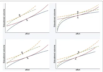
fixed level of school quality, and that student utility is increasing in the educational outcome and decreasing in effort. For a given level of school quality, students choose effort, and thereby (ignoring uncertainty) the educational outcome, to maximize util-ity. If school quality increases, education production possibilities increase for each level of effort. This is illustrated in Figure 1 for four different cases of production and util-ity functions. In each panel of Figure 1 the concave curves represent the education production functions before and after the increase in school quality (solid and dashed lines, respectively), and the convex curves are student indifference curves. The points marked by A are the initial utility maximizing choices of effort and outcome, and points marked by B are the corresponding choices after the increase in school quality. The ‘partial’ effect of an increase in school quality is given by the vertical shift of the produc-tion funcproduc-tion at point A (i.e., holding effort fixed at its initial optimal level). However, the upward shift in the production function implies that students may obtain a higher outcome with less effort. This ‘income effect’ tends to reduce effort. The substitu-tion effect may enhance the negative effort response if the marginal product of effort decreases when school quality increases, or it may work in the other direction if effort and school quality are complements in production. Of course, the optimal response of students also depends on the form of the utility function. The two left panels of Figure 1 illustrate cases where effort is reduced (more so in the upper panel) imply-ing that the total effect on the educational outcome is smaller than the partial effect. In the upper right panel, effort is unchanged (no difference between total and par-tial effect), and in the lower right panel effort is increased (the total effect exceeds the partial effect).

(5)

3 A parametric model

To fix ideas we consider a parametric model. We begin with the simplest case in which a student takes only one course.2The outcome is a marky. This mark is the result of school quality,s, student ability,μ, and student effort,h.3To make our main points as cleanly as possible we ignore uncertainty and take a simple parameterisation for the production function:

y=sλ+μhη+sλμhη (1)

Student effort and school quality are normalized so that 0<h< 1 and 0<s≤1. The parametersηandλcapture the curvature in the output with respect to student effort and school quality, respectively, andmeasures the degree of substitution or complementarity of the two inputs. To ensure that production is increasing and concave in both we assume that 0< λ <1, 0< η <1, >−1 and≥ −(μ)¯ −1, whereμ¯ is the maximum value of

μ. If <0 thensandhare substitutes in production, and if >0 they are complements. To motivate this function, note that education production may be considered to consist of two learning processes, learning at school (represented by the termsλ_{) and learning at} home doing homework (represented byμhη), and an interaction effect between the two processes represented by the last term in (1). The marginal effect of school resources may be smaller for well-prepared/high-ability students ( <0) if the primary goal of teaching is to ensure that all students obtain a basic level of skills. Also, the marginal effect of effort (and ability) may be smaller when school resources are high: when the learning process at school is more effective there may be smaller returns to effort at home to learning the curriculum. In conventional production functions including the Cobb-Douglas and CES functions, inputs are complements, i.e. the marginal product of one input (e.g.h) increases when the amount of the other input (s) is increased. However, as argued above,hands may be substitutes in production, so that the marginal product ofhis reduced whens increases, andvice versa.4

In empirical studies a parameter of interest isthe partial elasticityof the outcome with respect to school quality, holding effort constant:

= ∂lny

∂lns |h (2)

Note that in the parameterisation (1) the partial elasticity is not independent of effort and student ability. The same is true for the corresponding derivative∂y/∂s, unless= 0. If effort is fixed then we can recover the partial elasticity from observing variation inydue to experimental variation ins.

Typically neither experimental nor non-experimental studies of effects of school quality have access to data on student effort or time use, and therefore the interpretation of esti-mated effects as education production function parameters presumes that effort is fixed. However, it is perfectly reasonable to assume that some students might respond to the change in constraints with adjustment in effort expended. To capture this, let preferences be represented by the utility function:

u= y

1−σ

1−σ +δln(1−h) (3)

(6)

curvature in the concern about the outcome; higher values ofσgive a more kinked ben-efit function. That is, for higher values ofσ the student will have a high return below a threshold value ofy(‘passing’) and a low return above.

Denoting the optimal choices by

ˆ

h,yˆ

the total elasticityis given by:

ˆ

= dlnˆy

dlns (4)

Just as the partial elasticity is a parameter of interest in empirical studies, so is the total elasticity, which may be recovered by observing variation in the outcome (including vari-ation via effort response) due to experimental varivari-ation ins. However, in general, the total elasticity will not be equal to the partial elasticity. We define theelasticity differenceas

= ˆ− (5)

The sign of the elasticity difference will depend on the sign of the effort elasticity,

∂lnhˆ/∂lns. Clearly the elasticity difference will be positive ( > ˆ ) if the student responds to the increase in school quality by putting in more effort, and it will be negative if the effort elasticity is negative. Ifsandhare substitutes in production (≤0) the effort elasticity and the elasticity difference are negative. But if they are complements ( > 0) the marginal product of effort is increased when school quality increases, and therefore it may be optimal for the student to increase effort. Whether it is in fact optimal to increase effort depends on the size ofand the other parameters of the model, especially the cur-vature of the benefit function with respect to the outcome (σ). Thus, even ifsandhare complements it may still be optimal to reduce effort because of the ‘income effect’: an increase insenables students to obtain a largerywith less effort (more leisure).

First, we show that the effort elasticity (and therefore the elasticity difference) is nega-tive ifσ >1 or≤0. The marginal effect of school quality on effort is found by inserting (1) into (3) and differentiating the first-order condition:

∂hˆ

∂s = −

∂2u/∂hˆ∂s

∂2_u_/∂_hˆ2

∂2u

∂hˆ∂s =λs

λ−1_μη_hη−1_y−σ_[₍₁₋_{σ )}₋_σ_y−1_]

∂2u

∂hˆ2 =μηh

η−2₍₁₊_sλ₎_y−σ_[_(η₋₁₎₋_σ_y−1_μη_hη₍₁₊_sλ₎_]₋ δ

(1−h)2 <0 (6)

Thus, the sign of∂hˆ/∂sis equal to the sign of∂2u/∂hˆ∂s. It is obvious that∂hˆ/∂s< 0 if (≤0 and σ <1) or if (≥0 and σ >1). However,∂hˆ/∂sis also negative when <0 and σ >1. Thus, when <0 and σ >1 we have

∂2u

∂hˆ∂s <0⇔(1−σ )−σ (s

λ₊_μ_hη₊_sλ_μ_hη₎−1_<₀ ₍₇₎

⇔sλ+μhη+sλμhη< σ

1−σ

1

(8)

This inequality always holds given the assumed restrictions on the parameters. The RHS of the inequality tends towards its lower limit max(1,μ)from above whenσ → ∞and

(7)

(8) also holds (the derivative of the LHS with respect tois smaller than the derivative of the RHS). Thus,∂hˆ/∂s<0 if≤0 orσ >1.

We now examine further the determinants of the direction and size of the elasticity dif-ference . Although simple, the parametric model does not yield closed form expressions for the elasticities of interest. We therefore have to resort to simulations to illustrate how they vary with the parameters. Without loss of generality we can takeλ=0.4.6

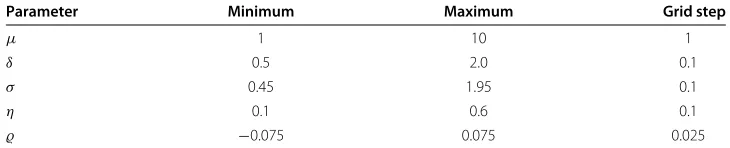
We take a grid over the values given in Table 1 (and calculate the elasticities ats=1).7

These values are, of course, wholly arbitrary and serve only to illustrate the variation in the elasticity difference. Since the maximum value ofμis here equal to 10, concavity is ensured when ≥ −0.1. For each set of parameter values, the partial elasticity is cal-culated holdinghfixed at the optimal level given the parameters and the initial level of school quality, whereas the total elasticity is calculated lettinghadjust to its new optimal level induced by the increase ins.

With this range of parameter values the minimum and maximum of the elasticity differ-ence are−0.12 and 0.00, respectively. Thus, even whenattains its maximum value of the grid (0.075) is not positive for any combination of the other parameters within the grid of Table 1. Table 2 shows that the parameter values that induce the extreme values of are very different. As expected, the largest negative value of is obtained whensand hare strong substitutes in production (attains its minimum). Also, is more negative if the benefit function is more curved (highσ), if the student has a higher taste for leisure (highδ), if the elasticity of output with respect to effort is high (highη), and/or if student ability (μ) is relatively low (although in this case not at its minimum).

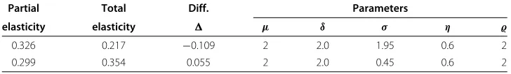
Whensandhare strong complements in production may be substantially positive. This is illustrated in Table 3 whereis fixed at 2. Here the largest negative value of is obtained for about the same values of (μ,δ,σ,η) as in Table 2 (except thatμis 2 instead of 3), whereas the largest positive value of (0.055) is obtained for the same parameter values except thatσ (the curvature of the benefit function) is at its minimum instead of its maximum.8

Within any school, we would expect that the parameters(μ,δ,σ,η,)are heteroge-neous. For example, how important it is to attain more than a simple ‘passing’ grade will vary from student to student, implying heterogeneity in the parameterσ. Moreover, the distributions of these parameters may not be independent. For example, high ability students (highμ) who aspire to further education may have a lower concern for simply passing.

4 Differential effects

The results of Summers and Wolfe (1977), Krueger (1999), Angrist and Lavy (1999), Browning and Heinesen (2007) and Heinesen (2010) indicate that reducing class size

Table 1 Simulation parameter values

Parameter Minimum Maximum Grid step

μ 1 10 1

δ 0.5 2.0 0.1

σ 0.45 1.95 0.1

η 0.1 0.6 0.1

(8)

Table 2 Extreme values of the difference between total and partial elasticities

Partial Total Diff. Parameters

elasticity elasticity μ δ σ η

0.249 0.125 ₋0.124 3 2.0 1.95 0.6 ₋0.075

0.062 0.062 −0.000 10 0.5 0.45 0.1 0.075

has larger positive effects for students from disadvantaged backgrounds, and Heinesen (2010) also finds that low-ability students benefit significantly more than high-ability stu-dents. Aaronson et al. (2007) find that teacher-quality effects are relatively larger for lower-ability students.

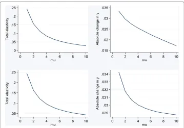
The simple model described above is consistent with these findings since the total elas-ticity,ˆ, is decreasing in student ability,μ. The absolute value of the total effect of school resources on marks (dyˆ/ds) is also decreasing inμfor many combinations of values for the other parameters. When = 0 (i.e., s andh are neither substitutes nor comple-ments in production), the derivative∂y/∂sin the production function (1) holdinghfixed does not depend onμ. However, the total effect∂yˆ/∂sdepends onμbecause students respond to changes in school quality by changing effort. This is illustrated in Figure 2 which shows howˆanddyˆ/dsvary withμin the model consisting of (3) and (1) where

(δ,σ,η)=(1.0, 1.05, 0.4). In the lower part of the figure=0, and the lower right panel shows thatdyˆ/dsis decreasing inμ. The lower left panel shows that the total elasticity decreases much more inμ. This is not surprising sinceydetermined by the production function (1) holdinghfixed and also the optimal valueyˆare strongly increasing inμ. In the upper part of the figure= −0.05 (i.e.,sandhare substitutes in production). Whereas the total elasticity varies withμin much the same way in the two parts of the figure,dyˆ/ds decreases much more in the upper part of the figure, wheresandhare substitutes, than in the lower part.

Figure 3 illustrates differential effects with respect to the parameters of the utility func-tion, i.e. the curvature with respect to the educational outcome (σ) and the taste for leisure (δ), given constant values of student ability (μ= 5) and the curvature of the production function with respect to effort (η=0.4). In the special case where =0, school quality (s) and effort (h) are neither substitutes nor complements in production, and the deriva-tive with respect tosin the production function, holdinghconstant, is equal toλsλ−1, i.e. independent of the initial levels ofhandy. Assuming λ = 0.4 ands = 1 as above and considering a 10% increase ofs, the partial effect onyis 0.04. This is represented by the horizontal line in the upper left panel of Figure 3, whereas the two downward slop-ing curves in this panel show the total effects forδ =0.5 (solid line) andδ = 2 (dashed line), respectively. Whereas the partial effect is constant, the total effect is decreasing in

Table 3 Extreme values of the difference between total and partial elasticities when school quality and effort are strong complements (rho=2)

elasticity elasticity μ δ σ η

0.326 0.217 ₋0.109 2 2.0 1.95 0.6 2

(9)

Figure 2 Total elasticity and absolute change in outcome when school resources are increased by 10%.The two upper panels are for rho= −0.05, the two lower panels are for rho=0.

bothσandδ. When bothσandδare small (about 0.5) the total effect is about 6% smaller than the partial effect; the difference is about 12% if insteadδis large (2); and it is about 40% ifσ is large (1.95). The upper right panel of Figure 3 shows the corresponding rela-tionship between the elasticity difference andσ for the two extreme values ofδ(and again for=0). The numerical value of the elasticity difference increases in bothσand

δ, and it is about−0.07 when both parameters are large (about 2) and in this case the partial elasticity is 0.16. The relation between the elasticity difference and the utility func-tion parameters is almost the same when= −0.05, i.e. whensandhare substitutes in production; see the lower left panel. The lower right panel shows the relation whensand hare strong complements ( = 2): whenσ is small the elasticity difference is positive (hincreases in response to the increase ins), and more so whenδis large; but whenσis large the elasticity difference is negative and large numerically (of about the same size as when=0 or= −0.05).

5 A pass/fail mark

If in this simple model the curvature parameter in the utility function is above a threshold (σ > 1), students respond to an increase in school quality bydecreasing their effort. Conversely, ifσ <1 (and >0), students may in some cases respond by increasing their effort. To investigate in more detail the effect of the curvature of the benefit function we consider an extreme case in which:

(10)

Figure 3 Differential effects with respect to parameters of the utility function: Total and partial effects and elasticity differences.

whereI(y≥y∗)is an indicator function that takes value unity ify≥y∗and zero otherwise (withy∗>sλ_{). This corresponds to a pass/fail mark. In this case students will either set:}

h=0⇒u=0

h=

y∗−sλ

μ(1+sλ₎

1 η

⇒u=1+δln

⎛ ⎝1−

y∗−sλ

μ(1+sλ₎

1 η

⎞

⎠ (10)

where we assume that the passing grade is attainable for some feasible level of effort: y∗<sλ+μ(1+sλ). The student chooses to exert effort if:

δ≤ −

⎛ ⎝ln

⎛ ⎝1−

y∗−sλ

μ(1+sλ₎

1 η

⎞ ⎠ ⎞ ⎠

−1

(11)

This illustrates that,ceteris paribus, a pass grade is more likely if complementarity in production, student ability or school quality are high or if the student has a low taste for leisure.9For a given level of school quality we have three groups of students: bad fails; marginal fails (students who failed but were close to choosing to pass) and passes. If we increase school quality then the bad fails continue to exert no effort and fail, the marginal fails increase their effort (the level given in (10) with the new level ofs) and pass students reduce their effort and still pass. Thus we have three different responses to the policy change: negative, zero and positive.

6 More than one course of study

(11)

Aaronsonet al.(2007) find significant effects of, e.g., both math and English teachers on math test scores, and Heinesen (2010) finds significant negative effects of course-specific class size on marks in the same course, but also indication of negative effects on marks in other courses. One possible mechanism which may explain these cross-course effects (or spill-over effects between courses) is student reallocation of effort between subjects. This may be illustrated by an extension of the above model framework to the more general case with more than one course of study. For simplicity, consider the case with two courses. We assume that the utility function is additive in the two outcomes (with the same curvature parameter) and leisure:

v= y

1−σ

1

1−σ +

y1₂−σ

1−σ +δln(1−h1−h2) (12)

whereyiandhiare the outcome (a mark) and student effort in subjecti, respectively. We allow student ability (μi) to differ between subjects, but for simplicity we assume that the other parameters in the two subject-specific production functions are identical, and we assume their form to be similar to (1):

yi=sλi +μihηi +sλiμihηi, i=1, 2 (13)

Denoting the optimal choices by (hˆ1,hˆ2,yˆ1,ˆy2) we may consider four total elasticities,

namely elasticities of the two outcomes with respect to each of the two school quality inputs:

ˆ ii=

dlnyˆi

dlnsi

, i=1, 2 (14)

ˆ ij=

dlnyˆi

dlnsj

, i,j=1, 2, i =j (15)

The two total ‘own resource’ elasticities in (14) consist of a direct effect of increased school resources in subjection academic outcome in the same subject and an indirect effect through changed effort in subjecti. The two total cross-elasticities (15) are different from zero if an increase in school resources in one subject induces students to change effort in the other subject. The partial own-resource elasticities,ii =∂lnyi/∂lnsi, consist of only the direct effect, holding effort fixed. The partial cross-elasticities,_ij=∂lnyi/∂lnsj,i =

j, are zero. The sign of each of the four elasticity differences ij = ˆij−ij(i,j= 1, 2) is equal to the sign of the corresponding effort elasticity∂lnhˆi/∂lnsj.

As in the model with only one course of study, the signs of the elasticity differences are mainly determined by the signs ofσ and. Thus, we now show thatdhˆi/dsi < 0 and

dhˆi/dsj > 0 (i,j = 1, 2;i = j) ifσ > 1 or ≤ 0. To see this, we insert the production functions (13) into the utility function (12) and differentiate the first-order conditions:

∂hˆi ∂si = −

∂2v

∂hˆi∂si ∂2v

∂hˆ2_j/D

∂hˆi ∂sj =

∂2v

∂hˆj∂sj ∂2v

∂hˆi∂hˆj /D

D= ∂

2_v

∂hˆ2₁

∂2v

∂hˆ2₂−

∂2v

∂hˆ1∂hˆ2

2

(12)

where

∂2v

∂hˆi∂si

=λsλ_i−1μ_iηhη_i−1y−_i σ[(1−σ )−σy−_i 1]

∂2v

∂hˆ2_i =Ai−

δ (1−h1−h2)2

, ∂

2_v

∂hˆ1∂hˆ2

= − δ

(1−h1−h2)2

Ai=μiηhηi−2(1+sλi)y−iσ[(η−1)−σy−i 1μiηhηi(1+sλi)] (17)

SinceAi < 0, we have∂2v/∂hˆ2i <0. Furthermore,D=A1A2−(A1+A2)δ/(1−h1−

h2)2>0. Thus,∂hˆi/∂si<0 and∂hˆi/∂sj>0 iff(1−σ )−σy−i 1<0, and this inequality holds ifσ >1 or≤0 by arguments similar to the one-course case.

If we take a grid over the same values of the parameters as given in Table 1, where now bothμ₁andμ₂vary between 1 and 10, we obtain the extreme values of the elasticity dif-ferences 11= ˆ11−11and 12= ˆ12and the associated parameters shown in Table 4.10

The ‘own resource’ elasticity difference 11has extreme values−0.12 and−0.00, and the

same is true for 22 (not shown in the table since the model is symmetric in the two

courses). The elasticity difference 11(and 22) vary with the parameters in basically the

same way as in the one-course case (except for the dependence on ability in the other subject): The extreme negative value is obtained whenσ,δandηare at their maximum, whenis at its minimum, and when ability in the two subjects is low (although not at the minimum); the maximum value (zero) is obtained when whenσ,δandηare at their minimum, whenis at its maximum, and when ability is at its maximum in the same subject and at its minimum in the other subject. The two cross elasticitiesˆ12 andˆ21

have extreme values−0.00 and 0.05. The extreme positive value ofˆ12is obtained when σ,ηandμ1are at their maximum values, and when,δ andμ2are at their minimum

values. Thus, the elasticity of outcome in one subject with respect to school resources in the other subject is high whenis negative and numerically large,σis high, ability in the first subject is high and ability in the other subject is low. The minimum ofˆ₁₂is obtained when=0 and whenσ,δ,μ1andμ2are high, andηis low.

Table 5 illustrates that when school quality and student effort are strong complements in production ( = 2 in the table) then the elasticity difference of 11may be

substan-tially positive (as for in the model with a single subject) andˆ12 may be substantially

negative. The maximum of 11is obtained whenσandδare small andηandμ1 andμ2

are high. The minimum ofˆ₁₂is obtained for the same parameter values, except thatμ₁

Table 4 Extreme values of differences between total and partial elasticities in model with two courses of study

elasticity elasticity μ1 μ2 δ σ η

11 ˆ11 11

0.253 0.131 −0.121 2 2 2.0 1.95 0.6 −0.075

0.049 0.049 −0.000 10 1 0.5 0.45 0.1 0.075

12 ˆ12 12

0.0 ₋0.001 ₋0.001 9 10 2.0 1.95 0.1 0.000

(13)

Table 5 Extreme values of differences between total and partial elasticities in model with two courses of study when school quality and effort are strong complements (rho=2)

elasticity elasticity μ1 μ2 δ σ η

11 ˆ11 11

0.237 0.169 −0.068 10 10 0.5 1.95 0.6 2

0.210 0.308 0.098 10 10 0.5 0.45 0.6 2

12 ˆ12 12

0.0 −0.069 −0.069 3 10 0.5 0.45 0.6 2

0.0 0.032 0.032 10 1 0.5 1.85 0.6 2

is small. However, Table 5 also shows that whenσis large, 11may be substantially

neg-ative andˆ₁₂may be substantially positive even whensandhare strong complements in production.

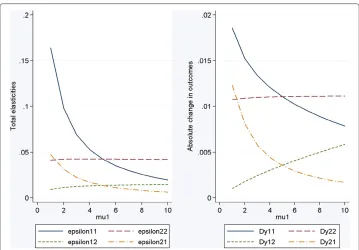
Figure 4 shows how the total elasticitiesˆij and the absolute change in the outcomes Dˆyij, which is the increase inyˆiwhensjis increased by 10%, vary with ability in subject 1 when(μ2,δ,σ,η,)= (5, 0.5, 1.95, 0.6,−0.05). Thus, the values ofδ,σ andηare chosen

so that the cross elasticities are relatively large. The own-subject elasticityˆ11 and the

absolute change Dyˆ11are decreasing inμ1corresponding to the results in the one-subject

case. The other own-subject elasticityˆ₂₂(and Dyˆ22) do not depend much onμ1, while the

cross elasticityˆ₂₁(and Dˆy21) are decreasing inμ1, andˆ12(and Dˆy12) are increasing inμ1.

The figure illustrates that the cross elasticities may be rather large compared to the own-subject elasticities. For instance, whenμ1 = 5 the cross elasticities are about one third

of the own-subject elasticities. Thus, when school resources in one course is changed, this may have substantial effects on outcomes also in other courses, and the mechanism

(14)

behind these cross effects in this simple model is students’ reallocation of effort between subjects: When school resources in one course increase it may be optimal for students to reduce effort in this course and increase leisure and effort in the other course. In Figure 4

= −0.05 so thatsiandhiare assumed to be substitutes in production. Settingequal to zero produces a rather similar figure although the cross elasticities are a little smaller compared to the own-course elasticities (forμ1 = 5 the ratio is 0.27). Assuming inputs

to be strong complements in production implies that the ratios of cross elasticities to own-course elasticities are smaller.

7 Conclusion

Typically, studies on the effect of school quality on academic outcomes do not take account of students’ responses regarding academic effort or time use. Applying simple parametric models we have shown that students’ effort or time-use responses to changes in school quality may cause large differences between the total elasticity of changes in school quality and the partial education production function elasticity (holding student effort constant). The main parameters determining the sign of the elasticity difference are the extent of substitution between effort and school quality in the production func-tion and how kinked is the benefit from a higher mark in the student utility funcfunc-tion. If effort and school quality are substitutes in production and/or if there is a marked kink in the benefit function, students will tend to reduce effort when school quality is increased implying that the total elasticity is smaller than the partial elasticity. The value of the elasticity difference also depends on the student’s distaste for effort, the curvature of the production function with respect to effort and the student’s ability in the course of study. In a model with two courses of study we have shown that an increase in school resources in one course may reduce effort in that course, implying that the total ‘own-resource elas-ticity’ is smaller than the partial own-resource elasticity, but increase effort in the other course implying a positive (total) ‘cross elasticity’.

Our main conclusion is that reliable estimates of partial effects (based on educa-tion produceduca-tion funceduca-tion parameters holding student effort constant) of school quality on academic outcomes require - in addition to exogenous variation in school quality - information on academic effort and/or time use. This suggests a new round of data collection.

(15)

8 Endnotes

1_{Studies on the effect of class size include, inter alia, Hanushek (1996), Krueger (1999,} 2003), Angrist and Lavy (1999), Case and Deaton (1999), Hoxby (2000), Krueger and Whitmore (2001), Heinesen (2010) and Fredriksson et al. (2013). Studies on the effect of teacher quality include Rockoff (2004), Rivkin et al. (2005), Aaronson et al. (2007) and Clotfelter et al. (2007a, 2007b, 2010). Other measures of school quality used in the literature include expenditure per student and the teacher-student ratio (see e.g. the surveys in Hanushek 1996, Card and Krueger 1996, and Betts 1996) and the number of teacher hours per student (Browning and Heinesen 2007).

2_{In the vastly simplified framework below we consider only a school that has one class.} A more general model would distinguish between class quality and school quality and allow for student selection based on within school quality differences.

3_{We use Greek letters to denote preference and prodcution parameters and Latin} letters to denote choice variables. Thussis the choice of the school funding authorities. As discussed in the Introduction, we ignore parental effort as an input in the production function which means that the model is more relevant for older students.

4_{Houtenville and Conway (2008) note that school resources and parental inputs may} be substitutes in education production.

5_{It is straightforward to allow for alternative uses of time such as market work. This} complicates the notation and analysis without adding much of significance to the main points.

6_{Results are qualitatively the same for other values of}_λ_.

7_{Choosing other values of}_s_{produces qualitatively similar results.}

8_{The production functions and indifference curves of Figure 1 are based on the} parametric model above and the four sets of parameters of Tables 2 and 3 (the upper panels of Figure 1 correspond to Table 2 and the lower panels to table 3).

9_{It is easily shown that} ∂ ∂s

y∗−sλ

μ(1+sλ₎

<0⇔1+y∗>0, and that this inequality holds because of the restriction≥ −1/μ.

10_{The elasticities are calculated at}_λ₌_{0.4 and}_s

1=s2=0.5.

Competing interests

The IZA Journal of Migration is committed to the IZA Guiding Principles of Research Integrity. The authors declares that they have observed these principles.

Acknowledgements

We are grateful to anonymous referees, the editor Pierre Cahuc, and Peter Fredriksson and participants in workshops on economics of education at Aarhus University for helpful comments and suggestions. The Danish Council for Strategic Research is acknowledged with gratitude for its support through the Centre for Strategic Research in Education (CSER).

Responsible Editor: Pierre Cahuc

Author details

1_{Oxford University, Manor Road, Oxford OX1 3UQ, England.}2_{Rockwool Foundation Research Unit, Sølvgade 10, DK-1307}

Copenhagen K, Denmark.

Received: 22 November 2013 Accepted: 29 January 2014 Published:

References

Aaronson D, Barrow L, Sander W (2007) Teachers and student achievement in the chicago public high schools. J Lab Econ 25(1):95–135

Angrist JD, Lavy V (1999) Using Maimonides’ rule to estimate the effect of class size on scholastic achievement. Q J Econ 114(2):533–575

Arcidiacono P, Aucejo EM, Spenner K (2012) What happens after enrollment? An analysis of the time path of racial differences in GPA and major choice. IZA J Lab Econ 1:5

Betts JR (1996) Is there a link between school inputs and earnings? Fresh scrutiny of an old literature. In: Burtless G (ed) Does Money Matter? The Effect of School Resources on Student Achievement and Adult Success. Brookings Institution, Washington DC, pp 141–191

Bonesrønning H (2004) The determinants of parental effort in education production: Do parents respond to changes in class size Econ Educ Rev 23:1–9

(16)

Card D, Krueger AB (1996) Labor market effects of school quality: Theory and evidence. In: Burtless G (ed) Does Money Matter? The Effect of School Resources on Student Achievement and Adult Success. Brookings Institution, Washington DC, pp 97–140

Case A, Deaton A (1999) School inputs and educational outcomes in South Africa. Q J Econ 114(3):1047–1084 Clotfelter CT, Ladd HF, Vigdor JL (2007a) How and why do teacher credentials matter for student achievement NBER

Working Paper No. w12828, http://www.nber.org/papers/w12828. Accessed 10 Jul 2012

Clotfelter, CT, Ladd, HF, Vigdor, JL (2007b) Teacher credentials and student achievement: Longitudinal analysis with student fixed effects. Econ Educ Rev 26:673–682

Clotfelter CT, Ladd HF, Vigdor JL (2010) Teacher credentials and student achievement in high school: a cross-subject analysis with student fixed effects. J Hum Resour 45(3):655–681

Das J, Dercon S, Habyarimana J, Krishnan P, Muralidharan K, Sundararaman V (2011) School inputs, household substitution, and test scores. NBER Working Paper No. w16830, http://www.nber.org/papers/w16830. Accessed 15 Sep 2012 Datar A, Mason B (2008) Do reductions in class size “crowd out” parental investment in education Econ Educ Rev

27:712–723

De Fraja G, Oliveira T, Zanchi L (2010) Must try harder: Evaluating the role of effort in educational attainment. Rev Econ Stat 92(3):577–597

Dustmann C, Rajah N, van Soest A (2003) Class size, education, and wages. Econ J 113:F99–F120 Fredriksson P, Öckert N, Oosterbeek H (2013) Long-term effects of class size. Q J Econ 128(1):249–285

Hanushek EA (1996) School resources and student performance. In: Burtless G (ed) Does money matter? The effect of school resources on student achievement and adult success. Brookings Institution Press, Washington, D.C, pp 43–73 Heinesen E (2010) Estimating class-size effects using within-school variation in subject-specific classes. Econ J

120:737–760

Houtenville AJ, Conway KS (2008) Parental effort, school resources, and student achievement. J Hum Resour 43(2):437–453 Hoxby C (2000) The effects of class size on student achievement: New evidence from population variation. Q J Econ

115:1239–1285

Krueger AB (1999) Experimental estimates of educational production functions. Q J Econ 114(2):497–532 Krueger, AB (2003) Economic considerations and class size. Econ J 113:F34–F63

Krueger AB, Whitmore DM (2001) The effect of attending a small class in the early grades on college-test taking and middle school test results: evidence from project STAR. Econ J 111:1–28

Lazear EP (2001) Educational production. Q J Econ 116(3):777–803

Rivkin S, Hanushek EA, Kain JF (2005) Teachers, schools, and academic achievement. Econometrica 73(2):417–457 Rockoff JE (2004) The impact of individual teachers on student achievement: evidence from panel data. Am Econ Rev

94(2):247–252

Summers AA, Wolfe BL (1977) Do schools make a difference Am Econ Rev 67(4):639–652

Todd PE, Wolpin KI (2003) On the specification and estimation of the production function for cognitive achievement. Econ J 113:F3–F33

Cite this article as:Browning and Heinesen:Study versus television.IZA Journal of Labor Economics