A Quantitative Method for Evaluating Reconstructed
One-Dimensional Bifurcation Diagrams
Yoshitaka Itoh, Masaharu Adachi*
Department of Electrical and Electronic Engineering, Tokyo Denki University, 5 Senju-Asachicho Adachi-ku, Tokyo , Japan.
* Corresponding author. Tel.: +81-3-5284-5407; email: adachi[at-mark]eee.dendai.ac.jp Manuscript submitted March 10, 2017; accepted June 8, 2017.
doi: 10.17706/jcp.13.3.271-278
Abstract: We describe a quantitative method for evaluating reconstructed 1-dimensional bifurcation diagrams. We estimate the oscillatory patterns of time-series data by reconstructing the bifurcation diagrams from time-series data alone. Such reconstruction can be used for real-world systems that have variable parameters, such as electric current and power, temperature, pressure, and concentration. In the conventional method, the reconstructed bifurcation diagram is qualitatively compared with the original one. Here, we evaluate the reconstructed 1-dimensional bifurcation diagrams by means of quantitative comparison with the original one. We also present the results of numerical experiments, demonstrating that our method is useful for quantitative evaluation of reconstructed bifurcation diagrams for the Hénon map and the Rössler equations.
Key words: Chaos, reconstruction of bifurcation diagram, time-series prediction, extreme learning machine, evaluation methods, levenshtein distance.
1.
Introduction
A bifurcation diagram (BD) is a visual summary of the succession for time-series data that are generated by a dynamical system as its parameters are varied. The oscillatory pattern of time-series data sometimes changes with a parameter. Here, the oscillatory patterns are periodic, quasi-periodic, and chaotic, and we estimate them by reconstructing the BDs. Such reconstruction could be used for real-world systems that have variable parameters, such as electric current and power, temperature, pressure, and concentration.
Tokunaga et al. proposed a method for reconstructing BDs from time-series data alone [1]. This method uses some of the time-series data that are generated by one dynamical system with some parameters. In addition, this method assumes that each parameter of the time-series data is close to the others. Moreover, it is better that these time-series show various oscillatory patterns. After it was first proposed, the method was studied further by several research groups [2]-[6].
two-dimensional BDs. We have previously proposed a method for estimating the Lyapunov spectra of reconstructed BDs [8]. We propose a method for quantitative evaluation of the reconstructed 1-dimensional BDs.
The rest of this paper is organized as follows. In Section II, we explain the reconstruction method applied to BDs. In Section III, we describe a method for evaluating the reconstructed 1-dimensional BDs. In Section IV, we present the results of our numerical experiments. Finally, we give conclusions in Section V.
2.
Procedure for Paper Submission
In this section, we describe the method for reconstructing a BD [1] using only some time-series data sets that are generated by one dynamical system with some parameters. Here, the time-series data set sn∈ ℝU is to be generated with parameter pn∈ ℝA, where U is the length of time-series data required for training and A is the dimensionality of the parameters. Therefore, time-series data sets s1, s2, ⋯ , sN correspond to parameter sets p1, p2, ⋯ , pN, respectively, where N is the number of time-series data sets. The algorithm is as follows.
1.We make a time-series predictor for each time-series data set 𝑠𝑛:
𝑦(𝑡 + 1) = 𝑃(𝑤𝑛, 𝑦(𝑡)), (1)
where
(𝑡) = [𝑦(𝑡) 𝑦(𝑡 ) ⋯ 𝑦(𝑡 ( 1) )] ,
(𝑡 + 1) = [𝑦(𝑡 + 1) 𝑦(𝑡 + 1) ⋯ 𝑦(𝑡 ( 1) + 1)]
Here, P(∙) is the time-series predictor, 𝑤𝑛 ∈ ℝ𝑊 is the set of trained connection weights for the time-series data sets 𝑠𝑛, k is the delay time, and 𝑦(𝑡) ∈ ℝ𝑌 and 𝑦(𝑡 + 1) ∈ ℝ𝑌 are the input and the output, respectively, of the time-series predictor. Terms and 𝑊 are the input and output
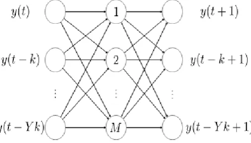
dimensionalities of the time-series predictor and the number of trained connection weights, respectively. In this paper, the dimensionality of output neurons is set to that of the input neurons in order to calculate the Jacobian matrix of the time-series predictor, which is used for estimating the Lyapunov exponents. In this paper, the dimensionality of the input and output neurons is set to that of the target dynamical system. We use an ELM as the time-series predictor. This is a feedforward neural network with a single hidden layer; the structure is shown in Fig. 1. The ELM is trained on only the connection weights of output neurons. The connection weights and biases of hidden neurons are initially generated as random values and then fixed.
2.We apply principal component analysis (PCA) to the trained connection weights 𝑤𝑛 of the time-series predictor. Eigenvectors 𝑢 ∈ ℝ𝑊, eigenvalues 𝜆
𝑖 ∈ ℝ(𝑖 = 1, ⋯ , 𝑊), estimated dimensionality 𝑄, and principal component coefficients γ ∈ ℝQ are obtained from the PCA. Here, we assume that 𝑄 is defined such that the 𝑄 th cumulative contribution ratio is the first to exceed 80%.
3.We reconstruct the BD by using the result of the PCA. A set of new connection weights is obtained:
̃ = [ 1 2 ⋯ ] + ̅ , (2)
where 𝑤̅ ∈ ℝ𝑊 is the average of the trained connection weights and 𝛾 is used as the parameter for
reconstructing the BD. The BD is reconstructed by repeatedly generating time-series data from new time-series predictors. Specifically,
(𝑡 + 1) = 𝑃( ̃ , (𝑡)), (3)
where the new connection weights 𝑤̃ are obtained for each parameter 𝛾 in the principal component
space.
4.We estimate the Lyapunov exponents of the reconstructed BD. Here, the Lyapunov exponent of each time-series predictor is estimated by using the methods of [9] and [10]. First, we calculate the Jacobian matrix of the time-series predictor P(∙) in (3) by using the method of [11]. Next, we decompose the Jacobian matrix by QR decomposition. Then, we obtain the Lyapunov exponents from
= l m
1
∑ lo (𝑡) 1
( = 1, ⋯ , ) (4)
where (t) is the jth diagonal component of a × real upper triangular matrix 𝑅(𝑡) obtained by QR decomposition and is the number of iterations.
3.
Evaluating Reconstructed 1-Dimensinal BDs
The proposed evaluation method is focused on the bifurcation structure. It compares the transition route from periodic to chaotic solutions, and the cycle number in windows. The BD is reconstructed by being expanded in some intervals and contracted in others. Therefore, this evaluation method does not consider the size of the cycle solution region or that of the chaotic region.
3.1.
Evaluation
cycle numbers in the reconstructed BD with those in the original BD.
3.2.
Levenshtein Distance
The Levenshtein distance [12] is a method for measuring the distance between two words. The distance between two words is defined as the minimum edit count required to change one word into the other, where edits are an insertion, deletion, or substitution. The algorithm is as follows.
Set O and H to be the cycle numbers for the original and the reconstructed BD, respectively. We
define f = [f1 f2 ⋯ fO] and = [ 1 2 ⋯ H] to be the sequential orders of cycle numbers in the original and reconstructed BDs, respectively.
Construct a matrix Υ ∈ ℝ(O+1)×(H+1).
Examine a cost Coh for every combination of fo from f and h from . If fo= h, then Coh= 0. If
fo≠ h, then Coh= 1.
Set cell υ[o, h] of the matrix Υ to the minimum value among the following: ∙ the cell immediately above plus one: υ[o 1, h] + 1,
∙ the cell immediately to the left plus one: υ[o, h 1] + 1,
∙ the cell diagonally above and to the left plus the cost: υ[o 1, h 1] + Coh.
Once steps iii and iv are complete, the Levenshtein distance is obtained from cell υ[O + 1, H + 1].
In this paper, the Levenshtein distance compares the chaotic regions and the sequential orders of the cycle numbers between the original and reconstructed BDs. Here, insertions, deletions, and substitutions refer to shortage, excess, and failure, respectively, of the cycle number or chaos in the reconstructed BDs.
4.
Simulation Experiments
We compare the Levenshtein distances of the reconstructed BDs of the Hénon map and Rössler equations with those of the original ones. For this experiment, we reconstruct the BDs from 5-, 7-, and 9-tuples of time-series data.
4.1.
Experimental Conditions for the Hénon Map
The Hénon map is given by
(𝑡 + 1) = (𝑡) + 1 2(𝑡), (5)
(𝑡 + 1) = (𝑡), (6)
where and are parameters and time-series data of (𝑡) are used for the reconstruction. These parameters are determined by
𝑛= 0 2 𝑠 (
2 ( 1)
1 ) + 1 2, (7)
= 0 3, (8)
where is the number of bifurcation paths (i.e., = 5, 7 or 9 in this experiment). We generate
time-series data 𝑠𝑛 for = 1, ⋯ , with 𝑛 as the of (5). We use 1,000 data from each time series
(𝑡 + 1) and (𝑡) for the output.
We define a range of parameters for comparison of reconstructed BDs with the structural features of the original BDs. The chosen range contains the transition route from periodic to chaotic solutions, as well as the periodic windows. For the BD of the Hénon map, we define the start point to be the period-doubling bifurcation from a 4-cycle to an 8-cycle, and the end point to be the first point at which the minimum value of the time-series data is less than -1.3. The parameter interval width ∆p ∈ ℝ is defined by
∆ = m n
( 𝑛 ) ( )
, (9)
where (start) and (end) are the parameter values at the start and end points, respectively, and is the number of parameters for the BD. In this experiment, we set to 3000.
4.2.
Result for the Hénon Map
(a)Original. (b)5-tuple.
(c)7-tuple. (d)9-tuple.
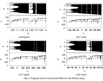
Fig. 2. Original and reconstructed BDs for the Hénon map.
Fig. 2 (a) shows the original BD of the Hénon map with the largest Lyapunov exponent.
Fig. 2 (b), (c), and (d) show the reconstructed BDs with the largest Lyapunov exponents that are generated from the 5-, 7-, and 9-tuple time-series data, respectively. The panels in each figure show the BD (upper) and the largest Lyapunov exponents (lower). Table 1 lists the Levenshtein distances of the reconstructed BDs in Fig. 2 (b), (c), and (d) relative to the original one in Fig. 2 (a). This shows that the more time-series data sets we use, the higher the reconstruction accuracy.
Table 1. Levenshtein Distances for the Hénon Map
4.3.
Experimental Conditions for the Rössler Equations
The Rössler equations are
= , (10)
= + , (11)
= ( ) , (12)
where , and are parameters and time-series data of are used for the reconstruction of the BDs. These parameters are determined by
n= 0 5 𝑠 (
2 ( 1)
1 ) + 3 7, (13)
υ = 0 33 (14)
= 0 3 (15)
where is the number of bifurcation paths (i.e., = 5, 7 or 9 in this experiment). We generate
time-series data 𝑠𝑛 for = 1, ⋯ , with 𝑛 as the of (12). We do so by using a third-order Runge-Kutta method with a time step of 𝛥𝜏 = 0 01. We use 5,000 data from each time series to train the time-series predictor. Here, one step for the predictor corresponds to 5Δ for the target system. For the Rössler equations, the numbers of input, hidden, and output neurons of the time-series predictor are 3, 50, and 3, respectively, and the delay time is set to be 16. Thus, the input and desired output relations of the time-series predictor are (𝜏), (𝜏 16 × 5𝛥𝜏), and (𝜏 32 × 5𝛥𝜏) for input; (𝜏 1 × 5𝛥𝜏), (𝜏 15 × 5𝛥𝜏), and (𝜏 31 × 5𝛥𝜏) for output. For the Rössler equations, we use a difference time
series as the desired output, applying the method proposed by [7].
For the BDs of the Rössler equations, we define the start point as the period-doubling bifurcation from periodicity 4 to periodicity 8, and the end point as the point at which the maximum value of the time-series data is more than 4.5.
4.4.
Results for the Rössler Equations
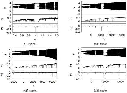
Fig. 3 (a) shows the original BD with its Lyapunov spectrum. Fig. 3 (b), (c), and (d) show the reconstructed BDs with the Lyapunov spectra that are generated from the 5-, 7-, and 9-tuple time-series data, respectively. In these figures, the upper panel shows the BD, and the middle and lower panels show the largest and second-largest Lyapunov exponents, respectively. In addition, we plot the local maxima of each time-series data set in the BDs.
We list the Levenshtein distances of Fig. 3 (b), (c), and (d) from Fig. 3 (a) in Table 2. This shows that the more time-series data sets we use, the more accurately the BD is reconstructed. This corresponds to a qualitative comparison of Fig. 3 (b), (c), and (d) against Fig. 3 (a). We see that Fig. 3 (d) looks the most like Fig. 3 (a).
5-tuple 7-tuple 9-tuple
(a)Original. (b)5-tuple.
(c)7-tuple. (d)9-tuple.
Fig. 3.Original and reconstructed BDs for the Rössler equations.
Table 2. Levenshtein Distances for the Rössler Map
5.
Conclusions
In this paper, we presented a method for quantitatively evaluating reconstructed 1-dimensional BDs. This method compares the chaotic regions and the sequential order of the cycle numbers between the original and reconstructed BDs, using the Levenshtein distance as a measure. We demonstrated that the results of the evaluation method agree with those from qualitative comparison. In addition, we showed that the more time-series data sets we used, the more accurately the BD was reconstructed. The results show that the proposed method is useful for the quantitative evaluation of reconstructed 1-dimensional BDs.
In future work, we will demonstrate the efficiency of this evaluation method for 1-dimensional BDs of other dynamical systems. In addition, we will attempt to evaluate BDs that are reconstructed by using other time-series predictors, and to develop a time-series predictor whose reconstruction accuracy is higher than that of the ELM.
References
[1] Tokunaga, R., Kajiwara, S., & Matsumoto, S. (1994). Reconstructing bifurcation diagrams only from time-waveforms. Physica, 79, 348-360.
[2] Ogawa, S., Ikeguchi, T., Matozaki, T., & Aihara, K. (1996). Nonlinear modeling by radial basis function networks. IEICE Trans,E79-A (10), 1608-1117.
[3] Bagarinao, E., Pakdaman, K., Nomura, T., & Sato, S. (1999). Reconstructing bifurcation diagrams from
5-tuple 7-tuple 9-tuple
noisy time series using nonlinear autoregressive models. Physica Review E, 60, 1073-1076.
[4] Bagarinao, E., Pakdaman, K., Nomura, T., & Sato, S. (1999). Time series-based bifurcation diagram reconstruction. Physica Review E, 130, 211-231.
[5] Bagarinao, E., Pakdaman, K., Nomura, T., & Sato, S. (2000). Reconstructing bifurcation diagrams of dynamical systems using measured time series. Method Inform. Med, 39, 146-149.
[6] Langer, G., & Parlitz, U. (2004). Modeling parameter dependence from time series. Physical Review E, 70,
1-9.
[7] Tada, Y., & Adachi, M. (2013). Reconstruction of bifurcation diagrams using extreme learning machines.
Proceedings of IEEE International Conference on Systems, Man, and Cybernetics (pp. 1127-1131).
[8] Itoh, Y., Tada, Y., & Adachi, M. (2015). Reconstruction of bifurcation diagrams with lyapunov exponents for chaoric systems from only time-series data. Proceedings of 2015 International Symposium on Nonlinear Theory and its Applications (pp. 692-695).
[9] Shimada, I., & Nagashima, T. (1979). A numerical approach to ergodic problem of dissipative dynamical systems. Prog. Theor. Phsy, 61 (6), 1605-1616.
[10]Sano, M., & Sawada, Y. (1985). Measurement of the lyapunov spectrum from chaotic time series. Phys. Rev. Lett., 55, 1082-1085.
[11]Adachi, M., & Kotani, M. (1979). Identification of chaotic dynamical systems with back-propagation neural networks. IEICE Trans. Fundamentals, E77-A(1), 324-334.
[12]Levenshtein, V. I. (1966). Binary codes capable of correcting deletions, insertions and reversals. Soviet physics doklady, 10, 707-710.
Yoshitaka Itoh is a doctoral student of graduate school of advanced science and technology, Tokyo Denki University, Japan. He received his master degree in engineering from Tokyo Denki University, Japan in 2011. He has worked at NEC informatec systems. His main research area is nonlinear time series prediction and analysis of chaotic system. He is a member of IEEE.