A Tableau Based Automated Theorem Prover
Using High Performance Computing
Md Zahidul Islam, Ahmed Shah Mashiyat
†, Kashif Nizam Khan, and S.M. Masud Karim
Computer Science and Engineering Discipline, Khulna University, Khulna, Bangladesh†Department of Mathematics, Statistics and Computer Science, St. Francis Xavier University, NS, Canada. Email: zahid@cse.ku.ac.bd, †x2008ooc@stfx.ca, kashif570@yahoo.com, and masud@cse.ku.ac.bd
Abstract— Automated Theorem Proving systems are enor-mously powerful computer programs capable of solving immensely difficult problems. The extreme capabilities of these systems lie on some well-established proof systems, such as Semantic tableau. It is used to prove the validity of a formula by contradiction and it can produce a coun-terexample if it fails. It can also be used to prove whether a formula is a logical consequence of a set of formulas. Tableau can be used in propositional logic, predicate logic, modal logic, temporal logic, and in other non-classical logics. In this article, we describe a detailed implementation of a sequential tableau algorithm for propositional and first-order logic using a procedural language rather then logic programming language. We also illustrate a tableau based proof system in a distributed environment using the Message Passing Interface. This paper also investigates two distinct approaches for parallel and distributed implementation and describes the experimental formula generation procedure. The proposed high performance approach will un-wrap an efficient paradigm for automated theorem proving.
Index Terms— Automated theorem proving, high perfor-mance computing, message passing interface, semantic tableau.
I. INTRODUCTION
In 1994, the famous “Pentium bug” caused Intel a loss of $475M [1]. Since then, formal verification of hardware and software has gained popularity in industry. There are two main approaches to formal verification: model checking and theorem proving. Model checking explores a (finite) model and theorem proving explores logical derivations of a theory. Automated theorem proving is the process of proving mathematical theorems by a computer program in an automated fashion. Automated theorem proving is currently the most well developed sub-field of automated reasoning. The language in which the math-ematical theorems or formulas are written is logic. As knowledge representation is often based on logic, many theorem provers have been successfully used to verify knowledge based systems [2]. More detail classification of verification approaches can be found in [3]. Among several theorem proving approaches, tableau is a widely used one. The main uses of the semantic tableaux method are validation check of a formula, to identify a logical consequence of a formula, and satisfiability checking of a set of formulas [4]–[6]. We discuss the tableau calculi for propositional logic, first-order logic and linear temporal
logic to describe our proposed theorem proving approach. Massive search space generated during automated rea-soning is considered as a critical problem in the field of theorem proving. Distribution and exploration of the search space in parallel is a motivating approach to handle this problem [7]. The aim of this paper is to investigate the scope of applying distributed memory computing to enhance the efficiency of theorem proving. This paper comprises the theoretical background, a description of the system architecture, details of the serial implementation and two different approaches to make it parallel. The proposed approach increases the memory capacity and the computing power by utilizing multiple processors of a cluster to manage the large search space.
The rest of the paper is structured as follows: section II introduces semantic tableaux, section III summarizes some existing tableau based theorem provers, section IV describes some implementation issues, section V de-scribes two different parallel implementations, and a case study with the proposed implementation is discussed in section VI. Finally, section VII points out some related ongoing research and future directions and concludes the paper.
II. SEMANTICTABLEAUX
The tableau method can be applied on both signed and unsigned formulas. Here we consider only the signed formulas. Signed formulas can be defined as, “A signed formula T φ is called true if φ is true and false if φ is false. And a signed formula F φ is called true if φ is false and false ifφis true”. The tableau method is based on the following eight facts. These facts hold under any interpretation of any formulasφandψ: (1) If¬φis true, thenφis false, (2) If ¬φis false, thenφis true, (3) If a conjunctionφ ∧ ψ is true, thenφ,ψ are both true, (4) If a conjunction φ ∧ ψ is false, then either φ is false or ψ is false, (5) If a disjunction φ ∨ ψ is true, then either φis true orψ is true, (6) If a disjunctionφ ∨ ψ is false, then φ,ψare both false, (7) If φ → ψ is true, then either φis false or ψis true, and (8) If φ → ψ is false, thenφis true and ψis false.
From the above facts we observe, there are two types of expansions - deterministic and nondeterministic. In a deterministic expansion, there is exactly one possible consequence (facts 1, 2, 3, 6 and 8). In a nondeterministic expansion, there is more than one possible consequence (facts 4, 5 and 7).
A. Tableaux Construction Rules
Based on the eight facts stated in earlier the tableau expansion rules, as in [6], are shown below in Figure 1. For each logical connective (¬, ∧, ∨, →), there are two rules: one preceded by the sign T and the other byF.
(1) a. T¬φ Fφ
b. F ¬φ
Tφ (2) a. T(φ ∧ ψ)
Tφ Tψ
b. F(φ ∧ ψ)
Fφ Fψ
(3) a. T(φ ∨ ψ)
Tφ Tψ
b. F(φ ∨ ψ) Fφ Fψ
(4) a. T(φ → ψ)
Fφ Tψ
b. F(φ → ψ) Tφ Fψ
Figure 1. Tableaux expansion rules for propositional logic
We can categorize these rules similarly as [6], cate-gory (A) those having direct consequences (T¬φ, F¬φ, T(φ ∧ ψ),F(φ ∨ ψ)andF(φ → ψ))and category (B) those having branches (F(φ ∧ ψ),T(φ ∨ ψ)and T(φ → ψ)).
While constructing a tableau, if a formula of type (A) occurs, we simultaneously subjoin its consequences into all branches below it. Similarly, when a formula of type (B) occurs, we divide all branches that pass through the line into sub-branches. Once we apply a rule to any formula, that formula is never expanded again.
B. Illustration of the Tableaux Method
Now let us see an example of tableau construction by applying the rules discussed so far. Let us consider, we wish to prove the formula φ = [p∨(q∧r)] → [(p∨ q)∧(q∨r)], wherep, q andr are atomic propositions. The complete tableau is given in Figure 2; explanation follows immediately. The number to the left of a line is used for identification purpose only; they are not needed in actual construction.
1. F[p ∨ (q ∧ r)] → [(p ∨ q) ∧ (p ∨ r)] 2. Tp ∨ (q ∧ r)
3. F(p ∨ q) ∧ (p ∨ r)
4. Tp
8. F(p ∨ q) 12. Fp 13. Fq
X
9. F(p ∨ r) 14. Fp 15. Fr
X
5. T(q ∧ r) 6. Tq 7. Tr
10. F(p ∨ q) 16. Fp 17. Fq
X
11. F(p ∨ r) 18. Fp 19. Fr
X
Figure 2. Tableau for the formulaφ = [p∨(q∧r)]→[(p∨q)∧(p∨r)]
To prove the formula, we need to drive a contradiction from the initial assumption that it is false. So we will start with the formula preceded by F. Now the formula is of the form F(φ → ψ) which is false only when φ is true and ψ is false (fact 8, rule 4(b)). We write (2) and (3) as a direct consequence of (1). Now (2) is of the formT(φ ∨ ψ), according to fact 5 (rule 3(a)) we cannot draw any direct conclusion from (2). Similarly, we cannot draw any conclusion from (3) (fact 4, rule 2(b)). So from (2) the tableau branches to two possibilities (4)T φ and (5)T ψ. Line (5) i.e.,T(q ∧ r)immediately producesT q andT r. Similarly when we explore all the formulas, we obtain the tableau tree in Figure 2.
Now at the left most branch (12) is a direct contradic-tion of (4). So we got a contradiccontradic-tion on this branch, and we can close this branch.
Similarly (14) contradicts (4), (17) contradicts (6), and (19) contradicts (7). Thus all branches are closed, i.e., they lead to a contradiction. Thus the formulaφ = [p∨ (q∧r)]→[(p∨q)∧(q∨r)] can never be false in any interpretation, so it is valid. The symbol ’X’ at the end of each branch indicates the corresponding branch is closed; we can close a branch as soon as a contradiction is found.
C. Tableau for First-Order Logic
Rule T∀: From T∀ xφ(x), we may directly infer T φ(a), where a is any parameter. Rule T∃: From T∃ xφ(x), we may directly infer T φ(a), where a is a new parameter i.e., has not been used yet. RuleF∀: From F∀xφ(x), we may directly inferF φ(a), whereais a new parameter as in RuleT∃. RuleF∃: FromF∃xφ(x), we may directly infer F φ(a), wherea is any parameter.
These four rules are shown in Figure 3.
RuleT∀: T∀xφ(x) T φ(a) (ais any parameter)
RuleF∃: F∃xφ(x) F φ(a) (ais any parameter)
RuleT∃: T∃xφ(x) T φ(a) (ais a new parameter)
RuleF∀: F∀xφ(x) F φ(a) (ais a new parameter) Figure 3. Tableaux expansion rules for first-order logic
Rules T∀ and F∃ are collectively called universal rules. Similarly Rules T∃andF∀ are collectively called existential rules. Decidability is a limiting factor in use of tableau method for first-order logic. For invalid formulas the tableau for first-order logic may lead to an infinite tableau. In fact, there is no correct and complete proof method for first-order logic that always terminates, as first-order logic is undecidable by definition. However in some cases (specifically when a branch represents a Hintkka set), the tableau method can decide whether a formula is invalid in the middle of the proof procedure.
D. Tableau for Linear Temporal Logic (LTL)
Efficient tableau-based methods for satisfiability testing and model checking of temporal formulae have been developed since the early 1980s: for the linear-time logic LTL (by Wolper [8]); for the branching-time logic UB (By Ben-Ari et al. [9]) and CTL (Emerson et al. [10]). Unlike automata-based approach for model checking and satisfia-bility checking of temporal logics, tableau-based methods are less developed and applied for industry applications, but are more natural and intuitive from logical perspective, easier for execution by humans, and (arguably) poten-tially more flexible and practically efficient, if suitably optimized [11]. Tableau based methods are one of the main methods for automating deduction in many temporal logics like LTL and CTL [12]. In this section we outline tableau based decision procedures for satisfiability of LTL formulae. For convenience of the reader not previously familiar with tableau-based decision procedures for LTL, we start our discussion with some preliminary concepts.
1) Syntax and semantics of LTL: LTL models time implicitly in along a path in the future. The syntax of LTL includes some temporal operators along with the propositional operators. The inductive definition of LTL in Backus Naur Form (BNF) is given below:
φ :=⊤ | ⊥ |p| ¬φ| (φ ∧ ψ)|(φ ∨ ψ)| (φ → ψ)| Xφ| F φ| Gφ|φ U ψ (1)
wherepranges over a finite set of proposition.
Many different semantics of LTL are available in liter-ature. We adopt the semantics discussed in [13]. In this framework LTL formulae are interpreted over a Kripke structure. LetM= (S,→, L(S))be such a structure and φis an LTL formula.π=s1→ · · · be a path inM. The semantics of LTL is defined as follows:
1) π|=⊤ 2) π6|=⊥
3) π|=piffp∈L(s1) 4) π|=¬φ iffπ6|=φ
5) π|= (φ∧ψ)iffπ|=φandπ|=ψ 6) π|= (φ∨ψ)iffπ|=φor π|=ψ
7) π|= (φ→ψ)iffπ|=ψ whenever π|=φ 8) π|=Xφ iffπ2
|=φ
9) π|=Gφiff∀i, i≥1, πi|=φ
10) π|=F φiff∃i, i≥1 such thatπi |=φ
11) π |= φU ψ iff ∃i, i ≥ 1 such that πi |= ψ and ∀j, j= 1,· · ·, i−1 we have πj|=φ
We writeπi for the path starting at si.
2) Tableau based decision procedure for LTL: Tableau for LTL is different than those for propositional and first-order logic. The complications in LTL tableau arise due to the fixpoint operators, as they require a special mechanism for checking realization of eventualities (the U operator). In LTL, Boolean connectives are handled similarly as for propositional logic and temporal connectives are handled by decomposing them into a requirement on the “current state” and a requirement on “the rest of the sequence”’. As discussed in [11], [12], [14], tableau for LTL requires the notion of Hintikka structures. Generally tableau for LTL involves two phases. In the first phase a tableau tree is constructed by applying tableau construction rules on the initial formula. Then in the second phase, the inconsistent nodes in the tree are removed from the tree. Inconsistent nodes are those not satisfying in any Hintikka structure. In LTL there are two types of inconsistencies - one is the propositional inconsistency (pand¬pin the same branch of the tableau tree) and the other one is any unfulfilled eventuality in a node. If the root node is removed during the second phase the initial formula is not satisfiable. Otherwise there is a Hintikka structure in the tableau tree satisfying the initial formula and therefore the initial formula is satisfiable. A convenient implementation direction of the tableau for LTL is available in [15].
III. EXISTING TABLEAU THEOREM PROVERS
In this section, we summarize some of the existing tableau theorem provers found in various literatures with an intention of providing a brief overview of the logic and the implementation language used.
A. 3TAP
B. Meteor
Meteor [17] compiles clauses into a data structure which is inferred by a sequential or parallel inference engine. The underlying inference mechanism of Meteor is model elimination with additional redundancy reducing mechanisms. It can prove first-order predicate logic in clausal form and developed using unix based C program-ming language.
C. Parthenon
Parthenon (PARallel THEorem prover for NON-Horn clauses) [18] is a parallel theorem prover for first-order predicate logic. The underlying proof calculus is a variant of model elimination. Parthenon is the first implemen-tation of an OR-parallel theorem prover, which runs on various multiprocessors capitalizing C-threading. It is implemented using a computational model similar to the SRI-Model for OR-parallel Prolog.
D. PTTP
The Prolog Technology Theorem Prover (PTTP) [19] is an implementation of the model elimination theorem-proving procedure. Instead of Prolog’s unbounded depth first search, it uses the depth-first iterative-deepening search to make the search strategy complete. It can prove theorems written in first-order predicate logic. This sequential theorem prover is implemented using Prolog and Lisp (Formally known as LISP).
E. SETHEO
The SEquential THEOrem prover SETHEO [20] is also based on the model elimination calculus. The tool ensures the completeness by iterative deepening using several depth measures. Based upon the efficient han-dling of syntactic un-equality constraints, a number of mechanisms for pruning the search space have been used in this tool. SETHEO is implemented using C and both sequential and parallel versions of SETHEO are available. Several parallel provers such as PARTHEO, SPTHEO and RCTHEO are developed on top of SETHEO.
F. LoTREC
LoTREC is a generic tableau theorem prover for modal logic. It is a suitable educational tool for students and researchers for creating, testing and analyzing tableau method implementations. LoTREC is sequential and de-veloped using Java [21] with an aim of flexibility, porta-bility, and nice interface.
G. MLTP
MLTP [22] implements a labeled tableau calculus, aim-ing to maximize both efficiency and generality. Several optimization techniques for modal logic reasoning are incorporated in MLTP. To facilitate generic reasoning, MLTP incorporates a generic data structure, a low-level macro language, an event-handler framework and a high-level specification language. MLTP is sequential and developed using C++.
H. FaCT++
Tableau method is also used as a reasoner for higher order logic. FaCT++ [23] is a tableaux-based reasoner for OWL Description Logics (DLs), implemented in C++. It can be used as a standalone DIG reasoner and as a back-end reasoner for the OWL API-based applications.
I. Pellet
Pellet [24] is an OWL DL reasoner based on the tableaux algorithms developed for Description Logics. Pellet is open-source and developed using Java. Pellet can be used with OWL API libraries and it provides a DIG interface.
IV. IMPLEMANTATION OF THE THEOREM PROVER
In this section, we discuss the issues related to se-quential implementation of the theorem prover including the syntax of formula representation, data structure, ex-pansion rule representation, terminating conditions, and the tableau construction algorithm. We also discuss two different approaches to make it parallel.
A. Syntax
The proposed algorithm takes the input represented by a string, and returns the tableau tree in inorder with the closed branches marked ’closed’. The implementation supports all the usual Boolean connectives represented as: and for ∧, or for ∨, implies for→ and not for¬. The formulas can be defined in BNF as:
φ := p|not φ|(φ and ψ)|(φ or ψ)|(φ implies ψ)
Where p stands for any atomic proposition and each occurrence of φto the right of:=stands for any already constructed formula.
B. Data Structures
1) Formula Representation: In our implementation, a formula is stored in a tree structure as in [13], [22]. Advantages of the tree structure include, easy extract-ing sub-formulas, which is, in fact, the most common operation during derivations; easy to verify that a for-mula is well formed; and obviously in a tree repre-sentation we do not need to search for an operator to apply an expansion rule, as it is the root of the formula tree. The tree representation of the formula (p or (q and r)) implies((p or q)and (p or r)) and the sub formulas after applying the expansion rule are depicted in Figure 4 and Figure 5.
2) Tableau Tree Representation: The tableau is a tree, made up of nodes. Every node of the tree contains the following fields.
leftNode: A pointer to the left subtree of the current node.
Figure 4. Tree representation of the formula
(p or(q and r))implies((p or q)and(p or r))
Figure 5. The two sub formulas after applying expansion rule
parentNode: A pointer to the parent of the current node.
formulaList:A pointer to the list of formulae of the current node.
closed: A boolean flag indicating whether the corresponding branch is closed or not.
The formulaListpointer in a tableau node points to a list where each node in the list is a formula with some additional information as follows.
index:A unique integer identifier for the node. sign: A boolean flag used to indicate the sign of the current formula.
formula: A pointer to the formula tree of the current node.
status:A boolean flag indicating whether the formula is processed or not.
Besides the two main data structures described above, some conventional data structures like list, stack and queue are used to manipulate the formula and tableau nodes.
C. Expansion Rules Representation
For simplicity, we used a unifying scheme as [4], [6], in our implementation. This scheme classifies formulae into two groups based on their logical connectives. Conjunc-tive type formulas are called α-formula and disjunctive
type formulas are calledβ-formula.αandβ-formulas are shown in Table I below.
TABLE I.
αANDβ-FORMULAS
α α1 α2 β β1 β2
T(φ ∧ ψ) T φ T ψ T(φ ∨ ψ) T φ T ψ F(φ ∨ ψ) F φ F ψ F(φ ∧ ψ) F φ F ψ F(φ → ψ) T φ F ψ T(φ → ψ) F φ T ψ T(¬φ) F φ F φ T(¬φ) F φ F φ F(¬φ) T φ T φ F(¬φ) T φ T φ
Using these α, β notations now we need only two expansion rules: if an α-formula occurs on a branch replaces it with α1 followed by α2 on same branch and if aβ-formula occurs on a branch split the branch in two, one with β1and other one with β2.
D. Terminating the Tableau Construction
It is very important to identify when to terminate the construction of the tableau tree. In our implementation, a tableau construction terminates in one of two cases: when all the branches are closed or when there is no more formula to process. A branch in the tableau tree closes as soon as a contradiction appears on that branch. A contradiction is of the form of a formula with both true and false sign (F φ,T φ) on the same branch. Thestatus of all the formulas is true (section IV.B.2) indicates there is no more formula to process. The closed is marked true (section IV.B.2) only if a contradiction is found.
E. The Tableau Algorithm
At the beginning, a tableau tree is constructed from the input formula. We define the root of the tableau tree with attributes leftNode, rightNode, parentNode, formulaList,closed. Initially, this tableau root node is added to a queue tableauNodeQueue. The algo-rithm skeleton is provided in Algoalgo-rithm 1.
Algorithm 1: TableauAlgorithm Data: Input formula.
Result: True or Counter Example begin
Instantiate formulaListnode with attributes: index←−0
sign←−f alse
formula←−a pointer to the input formula tree
status←−f alse
Instantiate the root node with attributes: leftNode←−null
rightNode←−null
parentNode←−null
formulaList←−a pointer to the formulaList
closed←−f alse
Add root node to tableauNodeQueue while tableauNodeQueue6=∅ ∨ all the branches are closed do
currentNode←− f ront(tableauN odeQueue)
for all formulas ∈formulaListof
currentNodedo
if α-formula then
Expand to two new sub formulas with status f alse
Add the new sub formulas to the end of formulaList
else
addβ−f ormulato betaFormulaQueue
for formulas ∈betaFormulaQueue do
if β-formula then
Expand the formula
create two new tableau nodes with parentNode←− currentNode Two formulas are added to
formulaListof newly created nodes
occurs whenever a branch closes. The tableau construction terminates when all the branches closes. To check this condition we need to search the whole tableau tree. To find contradiction, when a branch closes, the tableau tree starting at the root is searched in inorder.
F. The Tableau Algorithm for LTL
This section gives an informal algorithm for LTL tableau based on the discussion in section II-D.2. Our algorithm is analogous to the apporaches in [9], [15], [25]. The algorithm first constructs the tableau tree
ap-plying construction rules and then removes the incon-sistent nodes. The construction rules are defiend using Smullyan’s α-,β-notation given in Figure 6.
The construction starts with an LTL formula ϕ as the root. We use Uni to represent the set of formulas at a
node ni. Let n0 be the root of the tableau tree Tϕ, the construction begins withUn0={ϕ}. Following rules are then applied to construct the final tableau tree.
αrule:If α ∈ Un, then create a single child n1 of n withUn1 =Un∪ {α1, α2}
β rule:Ifβ∈Un, then create two childrennlandn2of
nwithUn1 =Un∪ {β1} andUn2 =Un∪ {β2} When any more application ofα,β rules is not possi-ble, the following X rule is applied.
X rule:If Xϕ∈Un, then create a single childn1 ofn withUn1 =Un∪ {ϕ}
Applications ofα-,β-rules (except for operators∧,∨) may create a node with same formulas. This situation is handled using a “feedback” edge instead of creating a new node. The construction ofTϕterminates by the following two rules.
T1: If {ϕ,¬ϕ} ∈ n, (this is same as the proposi-tional tableau) this node is closed and is not expanded further.
T2: If a nodemis about to be created as a child of a noden and there is an ancestorn′ ofn such thatU′
n=Um, then without creatingm,n and n′ are connected with a “feedback” edge. After the construction we apply the following rules to eliminate the unsatisfiable nodes of Tϕ.
E1: If{ϕ,¬ϕ} ∈n, then eliminaten.
E2: If all the successor of n have been eliminated, then eliminaten.
E3: IfXϕor ϕ U ϕ′ ∈n and
If there is no path inTϕfrom nton′ such that ϕ′ ∈n′, then eliminaten.
The decision procedure terminates after all unsatisfiable nodes have been eliminated. If the rootn0has been elim-inated, thenϕis not satisfiable otherwise it is satisfiable.
V. PARALLEL TABLEAU THEOREM PROVER
α α1 α2 β β1 β2
¬¬φ φ φ ¬(φ∧ψ) ¬φ ¬ψ
φ∧ψ φ ψ φ∨ψ φ ψ
¬(φ∨ψ) ¬φ ¬ψ φ U ψ ψ φ∧X(φ U ψ)
¬Xφ) X¬φ X¬φ ¬(φ U ψ) ¬ψ∧ ¬φ ¬ψ∧ ¬X(φ U ψ)
Gφ φ XGφ ¬Gφ) ¬φ ¬XGφ
Figure 6. αandβ-formulas for LTL.
implement the parallel version of the theorem prover. The intended architectures are discussed below. The following architectures are based on the Single Program Multiple Data (SPMD) model. Both the approaches are inspired by [7], [27].
A. Distributed Memory Computing
A distributed memory algorithm runs on many indi-vidual computers. Each computer processes a small piece of input data with its own computation resources. Com-munication between participating computers is needed to complete the computation for exchanging input data and computed results. There are several network primitives used by distributed processes to communicate with each other. The basic primitives are send and receive. A send message function provides a process the possibility to send a content of a block of memory to another process and allows the sender to put in a message type iden-tifier. The recipient of the message is specified by its logic identification rather than a physical address of the workstation. A receive function calls a block of memory with the content of a received message and supplies the receiving process with the enclosed tags to allow proper interpretation of the received data.
A computation of a distributed memory algorithm should terminate when the algorithm has reached a sit-uation that no process can progress further in the com-putation. We can ensure this by providing the fact that there is no message in transit. Unfortunately, to learn this, the processes need to communicate, i.e. to send and receive messages. This problem is generally referred to as a distributed termination detection problem in literature. For this reason we used two parallelizing technique to im-plement our parallel tableau algorithm. The first approach is a tree based approach where processes on the same branch communicate to detect termination. The second approach uses a centralized work pool where the master process keeps track of the terminated processes and each process notifies the master when it terminates.
B. Tree Based Partitioning Approach
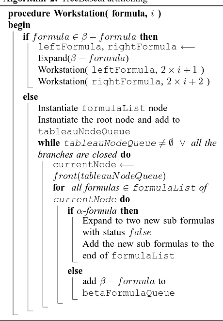
In this approach, the tree structure of the tableau is preserved. The root tableau node is assigned to the pro-cessor p0. Whenever a new node is created by processing a β-formula the left child node is sent to the processor 2×id+ 1 and right child is sent to 2×id+ 2, where id is the rank of parent processor as shown in Figure 7. The child processors can now work concurrently. The algorithm skeleton is provided in Algorithm 2.
Algorithm 2: TreeBasedPartitioning
procedure Workstation( formula, i) begin
if f ormula∈β−f ormulathen
leftFormula,rightFormula←− Expand(β−f ormula)
Workstation(leftFormula,2×i+ 1 ) Workstation(rightFormula,2×i+ 2 )
else
Instantiate formulaListnode Instantiate the root node and add to tableauNodeQueue
while tableauNodeQueue6=∅ ∨ all the branches are closed do
currentNode←− f ront(tableauN odeQueue)
for all formulas ∈formulaListof
currentNodedo
if α-formula then
Expand to two new sub formulas with statusf alse
Add the new sub formulas to the end offormulaList
else
addβ−f ormulato betaFormulaQueue
In case of searching, a processor can calculate its parent’s idusing the formulaf loor((id−1)÷2), where id is the rank of the child processor as depicted in Figure 8. The tree structure of the tableau construction made this approach an automatic choice.
C. Centralized Work Pool Approach
Figure 7. Parallel distribution of the tableau tree
Figure 8. Communication between the processors in searching
involves searching the local formula list only. A task queue is maintained by the master processor. Each slave processor only requests a new task when it is idle. The master sends the slave a task from the queue if the processed flag of the node is false. So a termination can be detected when all the slaves are idle and the processed flag of all the nodes in the task queue is true. To find out whether the input formula is satisfiable, the closedflag of the nodes in the task queue are checked. If the closed flag of all the nodes are true, we get a closed tableau, i.e., the input formula is satisfiable otherwise the formula is not satisfiable. A schematic view of the work pool approach is shown in Figure 9.
Figure 9. Centralized work pool distribution of the tableau tree
VI. CASE STUDY
In this section we describe our experimental results. We show a representation of reasoning about classical n-queen problem. The problem is to place n-n-queens on a
n × nchessboard so that no two queens dominate each other. In order to specify this problem we introduce n2 propositional variables; each associated with one square of the chess board. For convenience we show a toy exam-ple with only 4-queens. Figure 10(a) shows the solution to the problem; 10(b) shows an illegal configuration and 10(c) shows a legal configuration. Our implementation can conclude that (b) is illegal and (c) is legal by applying the tableau proof system discussed earlier.
A chess board is a 2D grid, where [1,2] represents the square at row 1 and column 2. Let us assume that the symbol q1,1 represents ”There is a queen in [1,1]”, then
¬q1,1 means ”There is no queen in [1,1]”. The rules of
4-queen can be represented as follows: Rule 1: At least one queen in row 1.
q1,1 ∨ q1,2 ∨ q1,3 ∨ q1,4
Similarly Rule 2, Rule 3 and Rule 4 are defined for row 2, 3 and 4.
Rule 5: At most one queen in row 1.
q1,1 → ¬q1,2 ∧ ¬q1,3 ∧ ¬q1,4
q1,2 → ¬q1,1 ∧ ¬q1,3 ∧ ¬q1,4
q1,3 → ¬q1,1 ∧ ¬q1,2 ∧ ¬q1,4
q1,4 → ¬q1,1 ∧ ¬q1,2 ∧ ¬q1,3
Rule 6, Rule 7 and Rule 8 for row 2, 3 and 4 are defined similarly.
Rule 9: At least one queen in column 1.
q1,1 ∨ q2,1 ∨ q3,1 ∨ q4,1
Similarly Rule 10, Rule 11 and Rule 12 are defined for column 2, 3 and 4.
Rule 13: At most one queen in column 1.
q1,1 → ¬q2,1 ∧ ¬q3,1 ∧ ¬q4,1
q2,1 → ¬q1,1 ∧ ¬q3,1 ∧ ¬q4,1
q3,1 → ¬q1,1 ∧ ¬q2,1 ∧ ¬q4,1
q4,1 → ¬q1,1 ∧ ¬q2,1 ∧ ¬q3,1
Rule 13, Rule 14 and Rule 15 for column 2, 3 and 4 are defined similarly. For diagonal positions the rules are defined as follows: No two queen can be diagonally dominating each other.
Rule 16: For a queen in [1,1].
q1,1 → ¬q2,2 ∧ ¬q3,3 ∧ ¬q4,4
Rule 17: For a queen in [1,2].
q1,2 → ¬q2,1 ∧ ¬q2,3 ∧ ¬q3,4
Rule 18: For a queen in [1,3].
q1,3 → ¬q2,2 ∧ ¬q3,1 ∧ ¬q2,4
Rule 19: For a queen in [1,4].
q1,4 → ¬q2,3 ∧ ¬q3,2 ∧ ¬q4,1
And so on... for other positions.
(a) (b) (c)
Figure 10. The 4-queen problem: (a) an actual solution; (b) an illegal configuration and (c) a legal configuration.
is a queen in [1, 2], the input is given in the following form:
φ:=F(KB ∧ q1,2 ∧ q2,1)
If this returns a closed tableau then we can concludeq2,1 is consistent with the KB i.e., a legal move. This rep-resentation using propositional logic is too tedius. Using first order logic the knowledgebase can be represented in a concise way. To represent the 4-queen problem using first-order logic, we made the following assumptions. Predicates: Queen(x, y)represents a queen in [x, y]. Constants: 1, 2, 3, 4 represents row and column numbers. Row constraints:
(i) At least one queen in each row.
∀i ∃j Queen(i, j)
(ii) At most one queen in each row.
∀i,j1,j2 Queen(i, j1) ∧ j1 6= j2 → ¬Queen(i, j2) Column constraints:
(i) At least one queen in each column.
∀i ∃j Queen(j, i)
(ii) At most one queen in each column.
∀i,j1,j2 Queen(j1, i) ∧ j1 6= j2 → ¬Queen(j2, i) Diagonal constraints:
At most one queen in [1,1], [2,2], [3,3] and [4, 4] . ∀i1,j1,i2,j2 Queen(i1, j1) ∧ i1 = j1
→ ¬ Queen(i2, j2)∧ i2 = j2 ∧ i1 6= i2 Similarly other constraints for all diagonal places can be defined. In this paper we show the tableau implementation for propositional logic only and we are wroking on it’s extension to first order logic. The tableau for first order logic is discussed in section II-C. We have tested our implementation with 8-queen, 9-queen and 10-queen problems. However due to lack of available resources we could not compare our results with other theorem provers. We wish to compare our results with others in future.
VII. CONCLUSION
This paper describes the requirements, issues, process, and implementation to develop a distributed tableau the-orem prover. Though our discussion is limited to propo-sitional, first-order, and LTL tableau only, this approach
can also be extended to other higher order logic. This type of parallel theorem prover is still not available, some earlier efforts can be found in [7], [27]. Though Prolog is a natural choice for the implementation of tableau al-gorithms, there are several difficulties in programming in Prolog. The highly unstructured nature of logic programs made it difficult to reuse the code. Extensive training is required for some new comer to understand the inner workings of a logic program written in Prolog. One of the key research problems in developing an automated theorem prover is to provide an easy to use interface to the user. Java suits well to provide the users with an easy to use interface to interact with the theorem prover, hiding the tedious details of the proof procedure. Considering these difficulties, we provide a framework that can be used to develop a tableau based algorithms using Java (or any high level programming language). In our previous work [28], we described the sequential implementation of the tableau theorem prover for only propositional logic and outlined two parallel approaches to make the theorem prover parallel. We have successfully developed the parallel versions of the proposed theorem prover and perform some experiments. In this paper, we provide a detailed description of building the test formulas which is used by the parallel theorem prover. Due to the tedious process of generating test formulas, we could not have sufficient formulas to provide a performance comparison of these two methods. In future, we wish to measure the performance of the two and identify the better one.
ACKNOWLEDGMENT
The authors wish to thank Kazi Shah Newaz Ripon for numerous discussions concerning this work, Abu Shamim Mohammad Arif and Kamrul Hasan Talukder for their assistance with implementation, and the anonymous reviewers of ICCIT 2010 for their valuable comments.
REFERENCES
[1] T. Coe, T. Mathisen, C. Moler, and V. Pratt, “Computa-tional aspects of the pentium affair,” IEEE Comput. Sci.
Eng., vol. 2, pp. 18–31, March 1995.
[3] D. Fensel, A. Schnegge, R. Groenboom, and B. Wielinga, “Specification and verification of knowledge-based sys-tems,” in Proceedings of the 10thBanff Knowledge Acqui-sition for Knowledge-Based System Workshop, 1996, pp.
18–20.
[4] M. Fitting, First-order logic and automated theorem
prov-ing (2nd ed.). Springer-Verlag New York, Inc., 1996. [5] M. D. Rijke, “Handbook of tableau methods, marcello
d’agostino, dov m. gabbay, reiner h¨ahnle, and joachim posegga, eds.” J. of Logic, Lang. and Inf., vol. 10, pp. 518–523, September 2001.
[6] R. M. Smullyan, Logical Labyrinths. A K Peters, Ltd., Wellesley, MA, USA, 2009.
[7] J. Schumann and R. Letz, “Partheo: a high-performance parallel theorem prover,” in Proceedings of the tenth
inter-national conference on Automated deduction, ser.
CADE-10. New York, NY, USA: Springer-Verlag New York, Inc., 1990, pp. 40–56.
[8] P. Wolper, “Temporal logic can be more expressive,” in
Proceedings of the 22nd Annual Symposium on Founda-tions of Computer Science. Washington, DC, USA: IEEE
Computer Society, 1981, pp. 340–348.
[9] M. Ben-Ari, Z. Manna, and A. Pnueli, “The temporal logic of branching time,” in Proceedings of the 8th ACM
SIGPLAN-SIGACT symposium on Principles of
program-ming languages, ser. POPL ’81. New York, NY, USA:
ACM, 1981, pp. 164–176.
[10] E. A. Emerson and J. Y. Halpern, “Decision procedures and expressiveness in the temporal logic of branching time,” in
Proceedings of the fourteenth annual ACM symposium on
Theory of computing, ser. STOC ’82. New York, NY,
USA: ACM, 1982, pp. 169–180.
[11] V. Goranko, “Temporal logics for specification and veri-fication,” in Proceedings of the European Summer School
in Logic, Language and Information (ESSLI’09), 2009.
[12] P. Abate, R. Gor´e, and F. Widmann, “One-pass tableaux for computation tree logic,” in Proceedings of the 14th
international conference on Logic for programming, arti-ficial intelligence and reasoning, ser. LPAR’07. Berlin, Heidelberg: Springer-Verlag, 2007, pp. 32–46.
[13] M. Huth and M. Ryan, Logic in Computer Science:
Mod-elling and Reasoning about Systems. New York, NY,
USA: Cambridge University Press, 2004.
[14] S. Schwendimann, “A new one-pass tableau calculus for pltl,” in Automated Reasoning with Analytic Tableaux and
Related Methods, ser. Lecture Notes in Computer Science,
H. de Swart, Ed. Springer Berlin / Heidelberg, 1998, vol. 1397, pp. 277–291.
[15] V. Goranko, A. Kyrilov, and D. Shkatov, “Tableau tool for testing satisfiability in ltl: Implementation and experimen-tal analysis,” Electron. Notes Theor. Comput. Sci., vol. 262, no. Elsevier Science Publishers B. V., pp. 113–125, May 2010.
[16] B. Beckert, R. H¨ahnle, P. Oel, and M. Sulzmann, “The tableau-based theorem prover 3tap version 4.0,” in
Pro-ceedings of the 13th International Conference on Auto-mated Deduction: AutoAuto-mated Deduction, ser. CADE-13.
London, UK: Springer-Verlag, 1996, pp. 303–307. [17] L. O. Astrachan and W. D. Loveland, “Meteors: High
performance theorem provers using model elimination,” Durham, NC, USA, Tech. Rep., 1991.
[18] S. Bose, E. Clark, D. Long, and S. Michaylov, “Parthenon, a parallel theorem prover for non-horn clauses,” in
Pro-ceedings of the Fourth Annual Symposium on Logic in
computer science. Piscataway, NJ, USA: IEEE Press,
1989, pp. 80–89.
[19] M. E. Stickel, “A prolog technology theorem prover: im-plementation by an extended prolog compiler,” in Proc. of
the 8th international conference on Automated deduction.
New York, NY, USA: Springer-Verlag New York, Inc., 1986, pp. 573–587.
[20] R. Letz, G. Stenz, and A. Wolf, “P-setheo: Strategy par-allel automated theorem proving,” in Proceedings of the
International Conference on Automated Reasoning with Analytic Tableaux and Related Methods (TABLEAUX-98), Lecture Notes in Computer Science, vol. 1397. Berlin-Heidelberg: Springer-Verlag, 1998, pp. 0–32.
[21] L. F. d. Cerro, D. Fauthoux, O. Gasquet, A. Herzig, D. Longin, and F. Massacci, “Lotrec: The generic tableau prover for modal and description logics,” in the
Pro-ceedings of the First International Joint Conference on
Automated Reasoning, ser. IJCAR ’01. London, UK:
Springer-Verlag, 2001, pp. 453–458.
[22] Z. Li, “Efficient and generic reasoning for modal logics,” Ph.D. dissertation, University of Manchester, Faculty of Engineering and Physical Sciences, School of Computer Science, 2008.
[23] D. Tsarkov and I. Horrocks, “Fact++ description logic reasoner: System description,” in Proc. of the Int. Joint
Conf. on Automated Reasoning (IJCAR 2006). Springer, 2006, pp. 292–297.
[24] E. Sirin, B. Parsia, B. Grau, A. Kalyanpur, and Y. Katz, “Pellet: A practical owl-dl reasoner,” Web Semantics:
Sci-ence, Services and Agents on the World Wide Web, vol. 5,
no. 2, pp. 51–53, 2007.
[25] P. Wolper, “The tableau method for temporal logic: an overview,” Logique et Analyse, 28(110–111), pp. 119–136, 1985.
[26] B. Carpenter, “mpijava home page,” available at url: http://www.hpjava.org/mpiJava.html. Last accessed: June, 2011.
[27] J. Schumann, “Sicotheo - simple competitive parallel the-orem provers based on setheo,” Parallel Processing for Artificial Intelligence 3, Machine Intelligence and Pattern Recognition, Tech. Rep., 1995.
[28] M. Z. Islam, A. S. Mashiyat, K. N. Khan, and S. M. M. Karim, “Towards a tableau based high performance au-tomated theorem prover,” in the 13th International
Con-ference on Computer and Information Technology (ICCIT 2010), 2010, pp. 406–411.
Md Zahidul Islam is currently a M.Sc.
stu-dent at StFX University, Antigonish, Canada. He received a B.Sc.Engg. degree in Computer Science and Engineering(CSE) from Khulna University, Bangladesh in 2007.
Currently he is working as a research as-sistant at CLI of StFX University, Canada. He is also a Lecturer at CSE Discipline of Khulna University, Bangladesh (now on study leave). After receiving his B.Sc.Engg. degree he has worked as a Part-time Lecturer at Khulna Uni-versity and as a software engineer at Dohatec New Media, Bangladesh. His areas of interest include formal verification, software engineering, and data mining.
Ahmed Shah Mashiyat has just finished his
Kashif Nizam Khan received his M.Sc in
Security and Mobile Computing under the Erasmus Mundus-NordSecMob Program from NTNU, Norway and AALTO (TKK), Finland in 2010. He received his B.Sc Engineering degree in Computer Science and Engineering from Khulna University in 2007. He has worked as a research assistant in AALTO and as a Lecturer in the Department of CSE in Ahsanullah University of Science and Technology and Khulna University. His research interests include information security, mobility management, formal verification, next generation mo-bile technologies (3G, 4G) and future internet.
S. M. Masud Karim has been serving as
![Figure 2. Tableau for the formula φ = [p∨(q∧r)] → [(p∨q)∧(p∨r)]](https://thumb-us.123doks.com/thumbv2/123dok_us/7824281.1665648/2.595.84.264.455.611/figure-tableau-the-formula-f-p-q-r.webp)