Improvement of BCI Performance Through
Nonlinear Independent Component Analysis
Extraction
Arjon Turnip and Dwi Esti Kusumandari
Technical Implementation Unit for Instrumentation Development, Indonesian Institute of Sciences, Bandung, Indonesia
Email: arjo001@lipi.go.id, jujhin@gmail.com
Abstract— Electroencephalogram (EEG) recordings provide an important means of brain-computer communication, but their classification accuracy and transfer rate are limited by unexpected signal variations due to artifacts and noises. In this paper, a nonlinear independent component analysis (NICA) extraction method for brain signal based EEG-P300 are proposed. The performance of the proposed method is investigated through a comparison of well known extraction methods (i.e., AAR, JADE, and SOBI algorithms). Finally, the promising results reported here reflect the considerable potential of EEG for the continuous classification of mental states.
Index Terms— Brain computer interface (BCI), Classification accuracy, Transfer rate, Nonlinear, ICA, Electroencephalogram (EEG).
I. INTRODUCTION
The human brain consists of approximately 1010 to 1011 neurons [1]. Signals between neurons are transmitted by means of action potentials, which are very short bursts of electrical activity. The total electric current produced in such a cluster is large enough to be detected by measuring the potential distribution on the scalp, which is the method used in electroencephalographic (EEG). EEG is used extensively for monitoring the electrical activity within the human brain, both for research and clinical purposes. EEG is used both for the measurement of spontaneous activity and for the study of evoked potentials. In particular the P300 evoked potential [2] is a positive peak that is evoked 300 ms stimulus onset. The presence, magnitude, topography, and time of the response signal are often used as metrics of cognitive function in decision making processes. In general, the detection of a P300 is made difficult by its low signal-to-noise (SNR) ratio compared to the ongoing background EEG.Human scalp EEG recording has the advantage of being noninvasive, inexpensive, and portable, which make it a very popular technique among the Brain computer interface (BCI) community [3-6].
Most EEG research seeks to understand the brain’s dynamic processes that are the basis of physical and mental activities. In addition to this, EEG signals are being investigated as a new mode of human-computer communication. If the information in a mental task is accurately obtained from EEG signals, a user can compose the sequence of the task to indicate commands that can operate a computer display or other devices. Successful operation of a BCI entails the user’s encoding of those commands in the EEG signals and the BCI’s subsequent derivation of the commands from the signals. Thus, a user and a BCI system need to be adapted to each other both initially and continually so as to ensure stable performance.
By extracting specific components from human brain activity and linking this brain activity to specifically developed algorithms, an interface between a computer and the users’ brain is created. Current BCI designs typically incorporate five main stages as shown in Fig. 1.Signals from the brain are processed to extract specific features that reflect the user’s intentions. Today there exist various techniques by which to accomplish this [7-12]. The user’s brain is now coupled to a computer or external device, which allow communication or controlling devices directly, without implementing any motor action. In this paper, a nonlinear independent component analysis (NICA) extraction method entailing time-series EEG signals is proposed. In order to examine the performance (i.e., accuracy and transfer rate) improvements of the proposed method, a classification using Fisher’s Linear Discriminant Analysis (FLDA) which has been well developed in the field of speech
Fig. 1.Basic design and operation of any BCI system. Manuscript received July18, 2013.
recognition is applied.
The contributions of this study are as follows.
(i) Enhancement and strengthening of artifacts-contaminated and stochastic EEG signals utilizing the small-amplitude of the EEG-P300.
(ii) Driving of the tracking error to a small value around zero while guaranteeing the closed-loop stability. (iii) Improvement of the classification accuracy and
transfer rate of a BCI by application of the proposed NICA method, even when subjects are in a fatigued condition.
The structure of the paper is as follows. Section II discusses the EEG data set and its preprocessing. Section III explains feature extraction and classification by the NICA method and the FLDA, respectively. Results are discussed in Section IV, and conclusions are drawn in Section V.
II. DATA SET AND EEG PREPROCESSING
The acquired signals are preprocessed to reduce external noises and detected artifacts. The filtered signals are then sent to the feature extraction and classification module, respectively. Since the purpose of this chapter is to demonstrate the performance of the compared extraction method, the present study utilizes the same raw data used in the work of Hoffmann et al., 2008 [13]. Also, only the data of 8 out of 32 channels (i.e., Fz, Cz, Pz, Oz, P7, P3, P4, and P8) placed at the standard positions described in the 10-20 International System [14] are used, which is claimed to be sufficient, in that a good compromise between the sufficiency of accuracy and the computational complexity in handling multiple channels is achieved.
The EEG signals were recorded at 2048 Hz sampling rate. The duration of each image flash (Fig. 2) was 100 ms, followed by a 300ms blank screen (i.e., the inter-stimulus interval was 400 ms). One trial takes about 400 ms; six trials make one segment; about 20~25 segments make one run; six runs make one session and four sessions are designed for individual subject. Therefore, one session involves 810 trials, and the entire data for one subject, therefore, was taken from an average of 3240 trials. Prior to feature extraction, several preprocessing operations including filtering and down-sampling were
carried out. To filter the data, a 6th-order band-pass filter (BPF) with cutoff frequencies of 1 Hz (i.e., to remove the trend from low frequency bands) and 12 Hz (i.e., to remove unimportant information in high frequency bands) was used.
It is difficult to compare the performances of the BCI systems, because the pertinent studies present the results in different ways. However, in the present study, the comparison was made based on the accuracy and the transfer rate. Accuracy is perhaps the most important aspect in any BCI. Besides accuracy, the transfer rate is also very important. The speed of a particular BCI is affected by the trial length, that is, the time needed for one selection. Thistime should be shortened in order to enhance a BCI’s effectiveness in communication. The bit rate (bits/trial) of eachselection can then be expressed as [15, 16].
1 1 log ) 1 ( ) ( log ) (
log2 2 2
N P P
P P N
b , (1)
Where N is a number of possible selections of the target and P denotes the probability that the desired choice is actually selected. The transfer rate (bits per minute) is equal to b multiplied by the average speed of selection S
(trial per minute, which is equal to the reciprocal of the average time required for one selection). Therefore, based on the data sets information, the desired output signal is developed.
III. FEATURE EXTRACTION AND CLASSIFICATION
A. Nonlinear Independent Component Analysis
The goal of feature extraction is to find data representations that can be used to simplify the subsequent brain pattern classification or detection.The extracted signals should encode the commands made by the subject but should not containnoises or other interfering patterns (or at least should reduce their level) that can impede classification or increase the difficulty of analyzing EEG signals. For this reason, it is necessary to design a specific extraction method that can reduce such artifacts in EEG records. Thus, the compared extractor are given to help the user for further research.
The M nonlinear mixed signals x1,,xM are related to N independent source signals s1,,sN through:
) , , (
) , , (
) , , (
1 1 2 2
1 1 1
N M
M
N N
s s f x
s s f x
s s f x
, (2)
which can be written in general form of ) (s f
x , (3)
Where x is the observed M-dimensional data (mixture) vector, f is an unknown real-valued M-component mixing function, and s is an N-vector whose elements are the N
unknown independent components. Assume now for simplicity that the number of independent components N
Fig. 2. The display used for evoking EEG-P300 signals [13].
equals the number of mixtures M. The general nonlinear ICA problem then consists of finding a mapping
N N
h: that gives components. To reconstruct the original signals, another nonlinear transformation is applied to x1,,xNto get y1,,yNthrough:
) , , (
) , , (
) , , (
1 1 2 2
1 1 1
N N
N
N N
x x h y
x x h y
x x h y
, (4)
or equivalently to
) (x h
y , (5)
that are statistically independent. A fundamental characteristic of the nonlinear ICA problem is that in the general case, solutions always exist, and they are highly non-unique. One reason for this is that if x and y are two independent random variables, any of their functions
) (x
f and g(y) are also independent. An even more serious problem is that in the nonlinear case, x and y can be mixed and still statistically independent. In the respective nonlinear ICA problem, one should find the original source signals s that has generated the observed data. An important special case of the general nonlinear mixing model (5) consists of so-called post-nonlinear mixtures. There each mixture has the form
n j
j ij i
i f a s
x
1
, i1,,n, (6)
Thus the sources sj,j1,,n are first mixed linearly according to the following basic ICA model
n
j j ja
s As x
1
, (7)
but after that a nonlinear function fi is applied to them to get the final observations xi. The goal is to find a specific model that explains how the observations were generated. In this study, the amounts to estimating both the source signals s and the unknown mixing mapping
) (
f that have generated the observed data x through the
general mapping (3).
Given m independent variables y(y1,,ym) and a
variable x, a new variable ym1g(y,x) is constructed
so that the set y1,,ym1 is mutually independent. The
construction is defined recursively as follows. Assume that we have already independent random variables
m
y
y1,, which are jointly uniformly distributed in
m ] 1 , 0
[ . Here it is not a restriction to assume that the distributions of the yi are uniform, since this follows directly from the recursion, as will be seen below; for a single variable, uniformity can be attained by the probability integral transformation. Denote by x any
random variable, and by a1,,am,b some nonrandom
scalars. Define
) , , (
, , ,
, , | ;
, , ,
1 1 ,
1 1 ,
1
m y
b
m x
y
m m x
y m
a a p
d a a p
a y a y b x P p b a a g
, (8)
where py() and py,x() are the marginal probability densities of y and (y,x), respectively, and P
| denotes the conditional probability. The py,x in the argument ofg is to remind that g depends on the joint probability distribution of y and x. For m0,g is simply the cumulative distribution function of x. Now, g as defined above gives a nonlinear decomposition.
A separation method for the post-nonlinear mixtures (5) should generally consist of two subsequent parts or stages: a nonlinear stage, which should cancel the nonlinear distortions fi,i1,,n. This part consists of
nonlinear functions gi
i,u
. The parameters iof each nonlinearitygi are adjusted so that cancellation is achieved. Alinear stage that separates the approximately linear mixtures v obtained after the nonlinear stage. This is done as usual by learning an
x
n
separating matrix Bfor which the components of the output vector yBv of the separating system are statistically independent.
Taleb and Jutten [17] use the mutual information
) (y
I between the components y1,,yn of the output vector as the cost function and independence criterion in both stages. For the linear part, minimization of the mutual information leads to the familiar Bell-Sejnowski algorithm [18]
1)
(
E xT BT
B y
I
, (9)
where components i of the vector
are score functions of the components yi of the output vectory
:) (
) ( ) ( log )
(
'
u p
u p u p du
d u
i i i
i
, (10)
Here pi(u)is the probability density function of yi and pi'(u) its derivative. For the nonlinear stage, one can derive the gradient learning rule [17]
n ik k k k ik i i
k k k k k
x g b y E
x g E y I
1 '
) , ( ) (
) , ( log )
(
, (11)
algorithm depends naturally on the specific parametric form of the chosen nonlinear mapping gk(k,xk). In [17], multilayer perceptron network (MLPN) is used for modeling the functions gk(k,xk),k1,,n.
In order to measure the performance of algorithms, we use the performance index (PI) as in [19, 20] defined by
n
i
n
k j ji
ki n
k j ij
ik
g g
g g
n n PI
1 1 1
1 max
1 max 1
1
(12) where G is the global transformation matrix from s to y,
gij is the (i,j) -element of the global system matrix G=HW and maxjgijrepresents the maximum value among the elements in the ith row vector of G, maxjgij does the maximum value among the elements in the ith column vector of G. When the perfect separation is achieved, the performance index is zero. In practice, the values of performance index around 10-2 gives quite a good performance.
B. Fisher’s Linear Discriminant Analysis
The goal in Fisher’s linear discriminant analysis (FLDA) is to compute a discriminant vector that separates two or more classes as well as possible. Here, we consider only the two-class case.We are given a set of input vectors xiD,i
1,,N
and correspondingclass-labels yi
1,1
Denoting by N1 the number oftraining examples for which yi =1, by C1 the set of indices
i for which yi= 1, and using analogous definitions for N2,
C2, the objective function for computing a discriminant
vector w[21]
2 2 2 1
2 2 1
) (
w
J , (13)
where
k
C i
i T
k
k w x
N 1
and 2
2
k C i
k i T
k w x
.
This means that one is searching for discriminant zectors that result in a large distance between the projected means and small variance around the projected means (small within-class variance). To compute directly the optimal discriminant vector for a training data set, matrix equations for the quantities
1
2
2 and
12
22 can be used. First, the class means of mk is defined
k C i
i k
k x
N
m 1 . (14)
Now we can define the between-class scatter matrix SB
and the within-class scatter matrix SW.
Tm m m
m1 2 1 2
B
S , (15)
k C i
T k i k i k
m x m x
2
1 W
S . (16)
With the help of these two matrices the objective function for FLDA can be written as a Rayleigh quotient.
w w
w w w J
T T
W B
S S )
( , (17)
By computing the derivative of J and setting it to zero, one can show that the optimal solution for w satisfies the following equation:
1 2
1 W
S m m
w . (18)
A potential problem in FLDA is that the within-class scatter matrix SW can become singular, and the inverse of
SW can become ill-defined. In particular, this happens when the number of features D becomes larger than the number of training examples N. A simple solution for this problem is to replace the inverse SW1 by the Moore– Penrose pseudo-inverse SW[22]. The output of FLDA given an input vector xˆ is simply the product wTxˆ . In
the P300-based BCI described in the present study, the output of FLDA was summed over trials and the image corresponding to the maximum of the summed output values was then selected.
IV. RESULTS AND DISCUSSION
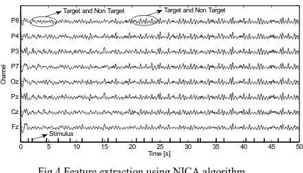
In this paper, a new method using nonlinear independent component analysis for extraxtion of EEG-P300 signals is proposed. The EEG signals were first preprocessed using a sixth-order band-pass filter (BPF) with cut-off frequencies of 1 Hz and 12 Hz, respectively, see Fig. 3. It can be seen that the signals were corrupted by noises. The feature extraction of the pre-processed signals of the eight electrodes (Fz, Cz, Pz, Oz, P7, P3, P4, and P8) can be compared with the extraction using NICA method in Fig. 4. The features were extracted every 400 ms interval (one trial) for about 120 target trials. From the results in Fig. 4, although the signals were still corrupted by noises (i.e., marked with high amplitude of non-target at some trials), the behaviors of the extracted signals clearly represent the EEG-based P300 evoked potentials (i.e., marked with higher amplitude of the target).
.
0 5 10 15 20 25 30 35 40 45 50
0 Fz Cz Pz Oz P7 P3 P4 P8
C
ha
nn
el
Time [s] Stimulus
.
0 5 10 15 20 25 30 35 40 45 50
Fz Cz Pz Oz P7 P3 P4 P8
C
ha
nn
el
Time [s]
Target and Non Target Target and Non Target
Stimulus
Fig.4 Feature extraction using NICA algorithm.
Plots showing the tracking error with and without application of the NICA approach aredrawn in Fig. 5. The curves indicate that with the NICA method, a level of
accuracy is attained after about 240
iterations.Contrastingly, when the proposed feature extraction method is not used, the same level of accuracy is attained only after 1800 iterations.These results show clearly that introduction of the NICA methods accelerates the training processes. The tracking error converges to a small value around zero,and the closed-loop stability is guaranteed. Furthermore, with the NICA algorithm, the convergence is faster.
In the present study, the performance of the proposed extraction method is tested using a FLDA classifier. In order to cope with nonlinearly separable problems, additional layers of neurons placed between the input layer and the output neuron are needed, leading to the multilayer perceptron architecture. At the outset, the structure of the network is chosen, after which the validation pattern appears in the graph window, and the network initialization values are introduced. Each subsequent layer has a weight coming from the previous layer. Performance is measured according to the specified performance function such as iteration speed and signal noise to ratio (SNR) criteria [23, 24]. The robustness of the proposedextraction algorithm was evaluated by comparing its separation performance with well-known algorithms (i.e., adaptive autoregressive model (AAR), jointapproximatediagonalization of eigenmatrices (JADE), and second-order blind identification(SOBI)) as shown in Fig. 6. Until all iteration, the NICA algorithm perform better performance index. This values indicate that the output of the proposed method gives better results for short training time. Fig. 7 shows typical performances of the comparative algorithms discussed in this paper.
0 500 1000 1500 2000 2500 3000
0 100 200 300 400 500 600
Epoch
Su
m
-S
qu
ar
ed
E
rro
r
Sum-Squared Network Error for 3000 Epochs
Fig. 5 Network’s performance according to mean square errors (ie., blue and red with and without NICA, respectively).
At high SNR, all tested algorithms perform very well. At low SNR, one can observe that the NICA method gives better performance than the other algorithms in most SNR ranges. In 0 - 4dB range SOBI is worse than the others.
The data sets for subject 5 were not included in the simulation since the subject misunderstood the instructions given before the experiment. Comparative plots ofthe classification accuracies and transfer rates (obtained with the others well known extraction method and averaged over four sessions based on the eight electrode configurations) for thedisable- (S1 - S4) and able-bodied subjects (S6 - S9) are depicted in Fig. 8 and Fig. 9, respectively. All of the subjects (using NICA extraction method), except for subject 9, achieved an average classification accuracy of 100% after five blocks of stimulus presentations were averaged (i.e., around 14 s). The reason for the poorer performance of subject 9 might be fatigue. Moreover, the performance of the proposed extraction method also can be seen in Fig. 10 (i.e., average of the disable subjects), Fig. 11 (i.e., average of the able-body subject), and Fig. 12 (i.e., average of all subjects). Those figures indicated that the proposed extraction method were superior compared to others extraction method. Shown alongside the classification accuracies for all of the subjects, in Table 1, are the corresponding 93%, 94%, 92%, and 96% confidence intervals corresponding to extraction methods using SOBI, JADE, AAR, and NICA, respectively.
0 500 1000 1500 2000 2500 3000 3500 4000 4500 5000
0 0.1 0.2 0.3 0.4 0.5 0.6 0.7
Number of iterations k
PI
(k
) [
dB
]
NICA AAR JADE SOBI
Fig. 6 Evolutions of PI(k) of the NICA, AAR, JADE, and SOBI algorithms.
-2 0 2 4 6 8 10 12 14 16 18
-102
-101
-100
SNR [dB]
Pe
rfo
rma
nc
e
In
de
x
NICA AAR JADE SOBI
Those values indicated that the results achieved through NICA method were highly superior compared to others method. If we analyze the results for accuracy (see Table 1), the disabled subjects obtained slightly better performance both with and without the proposed feature extraction method except with SOBI extraction. These results reflect the fact that the brain signals of the disabled subjects were less noisy and more homogeneous than those of the able-bodied subjects.
The transfer rates corresponding to the FLDA classification accuracies for the eight-electrode configuration were tested. The results showed that significant improvements in both classification accuracy and average transfer rate were obtained.The maximum average transfer rates, the mean transfer rates, and the standard deviations for all combinations of the featureextraction algorithm are listed in Table 2. These results show that the maximum average transfer rates for all of the subjects were much better with the proposed feature extraction method.
0 5 10 15 20 25 30 35 40 45 50
0 10 20 30 40 50 60 70 80 90 100 A c c u ra c y ( % ) Time (s)
0 5 10 15 20 25 30 35 40 45 50 0 5 10 15 20 25 30 35 40 45 50 0 5 10 15 20 25 30 35 40 45 50 0 5 10 15 20 25 30 35 40 45 50 Subject 1 Accuracy
Transfer rate
0 5 10 15 20 25 30 35 40 45 50
0 10 20 30 40 50 60 70 80 90 100
0 5 10 15 20 25 30 35 40 45 500
5 10 15 20 25 30 35 40 45 50
0 5 10 15 20 25 30 35 40 45 500
5 10 15 20 25 30 35 40 45 50
0 5 10 15 20 25 30 35 40 45 500
5 10 15 20 25 30 35 40 45 50
0 5 10 15 20 25 30 35 40 45 500
5 10 15 20 25 30 35 40 45 50 Tr a n s fe r ra te ( b it s /m in ) Subject 2
0 5 10 15 20 25 30 35 40 45 50
0 10 20 30 40 50 60 70 80 90 100 A c c u ra c y ( % ) Time (s)
0 5 10 15 20 25 30 35 40 45 500
5 10 15 20 25 30 35 40 45 50
0 5 10 15 20 25 30 35 40 45 500
5 10 15 20 25 30 35 40 45 50
0 5 10 15 20 25 30 35 40 45 500
5 10 15 20 25 30 35 40 45 50
0 5 10 15 20 25 30 35 40 45 500
5 10 15 20 25 30 35 40 45 50 Subject 3
0 5 10 15 20 25 30 35 40 45 50
0 10 20 30 40 50 60 70 80 90 100 Time (s)
0 5 10 15 20 25 30 35 40 45 500
5 10 15 20 25 30 35 40 45 50
0 5 10 15 20 25 30 35 40 45 500
5 10 15 20 25 30 35 40 45 50
0 5 10 15 20 25 30 35 40 45 500
5 10 15 20 25 30 35 40 45 50
0 5 10 15 20 25 30 35 40 45 500
5 10 15 20 25 30 35 40 45 50 Tr a n s fe r ra te ( b it s /m in ) NICA AAR SOBI JADE Subject 4 Accuracy Transfer rate
Fig. 8 Comparison of classification accuracy and transfer rate plots (averaged over four sessions based on eight electrode configurations)
for disabled subjects (subjects 1- 4).
0 5 10 15 20 25 30 35 40 45 50
0 10 20 30 40 50 60 70 80 90 100 A c c u ra c y ( % )
0 5 10 15 20 25 30 35 40 45 50 0 5 10 15 20 25 30 35 40 45 50 0 5 10 15 20 25 30 35 40 45 50 0 5 10 15 20 25 30 35 40 45 50 Subject 6
0 5 10 15 20 25 30 35 40 45 50
0 10 20 30 40 50 60 70 80 90 100
0 5 10 15 20 25 30 35 40 45 500
5 10 15 20 25 30 35 40 45 50
0 5 10 15 20 25 30 35 40 45 500
5 10 15 20 25 30 35 40 45 50
0 5 10 15 20 25 30 35 40 45 500
5 10 15 20 25 30 35 40 45 50
0 5 10 15 20 25 30 35 40 45 500
5 10 15 20 25 30 35 40 45 50 Tr a n s fe r ra te ( b it s /m in ) Subject 7
0 5 10 15 20 25 30 35 40 45 50
0 10 20 30 40 50 60 70 80 90 100 A c c u ra c y ( % ) Time (s)
0 5 10 15 20 25 30 35 40 45 50 0 5 10 15 20 25 30 35 40 45 50 0 5 10 15 20 25 30 35 40 45 50 0 5 10 15 20 25 30 35 40 45 50 Subject 8
0 5 10 15 20 25 30 35 40 45 50
0 10 20 30 40 50 60 70 80 90 100 Time (s)
0 5 10 15 20 25 30 35 40 45 500
5 10 15 20 25 30 35 40 45 50
0 5 10 15 20 25 30 35 40 45 500
5 10 15 20 25 30 35 40 45 50
0 5 10 15 20 25 30 35 40 45 500
5 10 15 20 25 30 35 40 45 50
0 5 10 15 20 25 30 35 40 45 500
5 10 15 20 25 30 35 40 45 50 Tr a n s fe r ra te ( b it s /m in ) NICA AAR SOBI JADE Subject 9 Accuracy Transfer rate
Fig.9 Comparison of classification accuracy and transfer rate plots (averaged over four sessions based on eight electrode configurations)
for able-bodied subjects (subjects 6- 9).
0 5 10 15 20 25 30 35 40 45 50
0 10 20 30 40 50 60 70 80 90 100 A c c u ra c y ( % ) Time (s)
0 5 10 15 20 25 30 35 40 45 50
0 5 10 15 20 25 30 35 40 45 50
0 5 10 15 20 25 30 35 40 45 50
0 5 10 15 20 25 30 35 40 45 50
Tr a n s fe r ra te ( b it s /m in ) NICA AAR SOBI JADE Averages of subject 1-4 Accuracy Transfer rate
Fig. 10 Average of classification accuracy and transfer rate plots for disabled subjects.
0 5 10 15 20 25 30 35 40 45 50
0 10 20 30 40 50 60 70 80 90 100 A c c u ra c y ( % ) Time (s)
0 5 10 15 20 25 30 35 40 45 50
0 5 10 15 20 25 30 35 40 45 500
5 10 15 20 25 30 35 40 45 50
0 5 10 15 20 25 30 35 40 45 500
5 10 15 20 25 30 35 40 45 50
0 5 10 15 20 25 30 35 40 45 500
5 10 15 20 25 30 35 40 45 50 Tr a n s fe r ra te ( b it s /m in ) NICA AAR SOBI JADE Averages of subject 6-9 Accuracy Transfer rate
Fig. 11 Average of classification accuracy and transfer rate plots for disabled subjects.
0 5 10 15 20 25 30 35 40 45 50
0 10 20 30 40 50 60 70 80 90 100 A c c u ra c y ( % ) Time (s)
0 5 10 15 20 25 30 35 40 45 50
0 5 10 15 20 25 30 35 40 45 500
5 10 15 20 25 30 35 40 45 50
0 5 10 15 20 25 30 35 40 45 500
5 10 15 20 25 30 35 40 45 50
0 5 10 15 20 25 30 35 40 45 500
5 10 15 20 25 30 35 40 45 50 Tr a n s fe r ra te ( b it s /m in ) NICA AAR SOBI JADE Averages of all subject Accuracy Transfer rate
Fig. 12 Average of classification accuracy and transfer rate plots for all subjects.
the BCI-applicability of the proposed extraction method. By contrast, the classification accuracies and transfer rates obtained using the well known extraction methods separately were found to be only marginally superior to mere chance, indicating the inadequacy of those methods for BCI applications.
One negative characteristic of P300 detection is that the amplitude of the waveform requires the averaging of multiple recordings to isolate a signal. In order tostreamline the averaging process, the proposed feature extraction modules were applied to segments of EEGsignals (EEG trials). These modules are integral to the classification accuracy and transfer rate of the mental activities. A factor relating to the attainment of good classification accuracy and transfer rates for disabled subjects, both in communication systems and BCI systems, is the sequence of a given stimulus. When applying the proposed method to extract EEG signal features, it was found that any two sequential target stimuli excite just one P300 component peak, and are extracted in that form. However, in orderthat EEG signals be classified with 100% accuracy, such stimuli must excite two peaks of amplitude. Therefore, in order to obtain a good classification accuracy and transfer rate, the given stimulus must be inputted randomly with a constraint. In other words, two targets should not be flashed sequentially.
TABLE 1.
AVERAGE CLASSIFICATION ACCURACY (%)
Subject SOBI JADE AAR NICA
S1 94.00 93.00 88.75 94.50
S2 92.25 94.50 90.00 97.30
S3 94.00 95.50 95.00 97.70
S4 93.00 94.25 94.50 97.25
S6 90.50 91.85 90.55 96.50
S7 94.75 94.00 93.20 96.25
S8 94.75 96.00 94.50 96.35
S9 93.70 92.95 90.00 97.50
Average
(S1–S4) 93.30.8 94.31.0 92.13.1 96.71.4 Average
(S6-S9) 93.42.0 93.71.7 91.12.1 96.60.5 Average
(all) 93.41.4 94.01.3 92.12.4 96.61.0
TABLE 2. AVERAGE TRANSFER RATE (%)
Subject SOBI JADE AAR NICA
S1 17.13 17.13 8.13 17.13
S2 12.58 17.48 10.60 34.96
S3 17.48 25.17 25.17 34.96
S4 11.77 17.13 17.48 34.96
S6 10.60 17.13 20.95 25.17
S7 17.13 17.13 17.13 25.17
S8 25.17 25.17 20.95 19.34
S9 17.13 17.13 17.13 34.96
Average
(S1–S4) 14.7 2.9 19.2 3.9 15.37.6 30.5 8.9 Average
(S6-S9) 17.5 5.9 19.1 4.0 19.02.2 26.26.4 Average
(all) 16.14.6 19.13.6 17.25.5 28.3 7.5
V. CONCLUSION
The results presented in this study show that, compared with the well known extraction algorithms, a better extraction result can be obtained when using the NICA algorithm (i.e., faster training and higher SNR) for single-trial ERPs based on the P300 component from specific brain regions. With NICA extraction, the data indicate that a P300-based BCI system can communicate at the rate around34.96 bits/min for the dis and able-bodied subjects. The average of 100% classification accuracy is achieved after four blocks (average) for disabled subjects and after five blocks (average) for able-bodied subjects. To improve our results, we are currently investigating the effect of averaging the output of the classifier over the consecutive windows as well as the effects of other preprocessing methods in artifact-effect reduction.
REFERENCES
[1] E. R. Kandel, J. H. Schwartz, and T. M. Jessel, editors, The Principles of Neural Science, Prentice Hall, 3rd edition, 1991.
[2] S. Sutton, M. Braren, E. R. John, andJ. Zubin, “Evoked potential correlates of stimulus uncertainty,”Science, vol.150, no. 700, pp. 1187-1188, 1965.
[3] E. Donchin, K. M. Spencer, and R. Wijesinghe, “The mental prosthesis: Assessing the speed of a P300-based brain–computer interface,”IEEE Trans. Rehabil. Eng., vol. 8, no. 2, pp. 174-179, 2000.
[4] G. Pfurtscheller, C. Neuper, A.Schlogl, and K.Lugger, “Separability of EEG signals recorded during right and left motor imagery using adaptive autoregressive parameters,”IEEE Trans. Rehabil. Eng., vol. 6, no. 3, pp. 316-325, 1998.
[5] F. Aloise, F.Schettini, P.Arico, F.Leotta, S.Salinari, D. Mattia, F.Babiloni, F.Cincotti, “P300-based brain-computer interface for environmental control: An asynchronous approach,”Journal of Neural Engineering, vol. 8, no. 2, 025025, 2011.
[6] A. Belitski, J. Farquhar, and P.Desain, “P300 audio-visual speller,”Journal of Neural Engineering, vol. 8, no. 2, 025022, 2011.
[7] M. Arnold, U. Moller, and H. Witte, “Nonlinear time-series modeling by means of self-exciting threshold AR models,”Theory in Biosciences, vol. 118, no. 3-4, pp. 261-266, 1999.
[8] H. Cecotti and A. Graser, “Convolutional neural networks for P300 detection with application to brain-computer interfaces,”IEEE Trans. Pattern Anal. Mach. Intell., vol. 33, no. 3, pp. 433-445, 2011.
[9] Z.-G. Che, T.-A. Chiang,and Z.-H. Che, “Feed-forward neural networks training: A comparison between genetic algorithm and back-propagation learning algorithm,”Int. J. Innov. Comp. Inf. Control, vol. 7, no. 10, pp. 5839-5851, 2011.
[10] J. Escudero, R. Hornero, D.Abasolo, A. Fernandez, “Quantitative evaluation of artifact removal in real magnetoencephalogram signals with blind source separation,”Annals of Biomedical Engineering, vol. 39, no. 8,pp. 2274-2286, 2011.
[12] A. Turnip, K.-S.Hong,and M.-Y.Jeong, “Real-time feature extraction of P300 component using adaptive nonlinear principal component analysis,”BioMedical Engineering OnLine, vol. 10, no. 83, 2011.
[13] U. Hoffmann, J.-M. Vesin, and T. Ebrahimi. An efficient P300-based brain–computer interface for disabled subjects.
Journal of Neuroscience Methods, vol. 167, no. 1, pp. 115-125, 2008.
[14] H. H. Jasper, “ Report of the committee on methods of clinical examination in electroencephalography,”
Electroenceph. Clin. Neurophysiol.,vol. 10, pp. 370-375, 1958.
[15] E. W. Sellers, D. J. Krusienski, D. J. McFarland, T. M. Vaughan, and J. R. Wolpaw,“A P300 event-related potential brain-computer interface (BCI): The effects of matrix size and inter stimulus interval on performance,”Biological Psychology, vol. 73, no. 3, pp. 242-252, 2006.
[16] J. R. Wolpaw, H. Ramoser, D. J. McFarland, and G. Pfurtscheller, “EEG-Based Communication: Improved Accuracy by Response Verification,”IEEE Trans. On Rehab Eng., vol. 6, no. 3, pp. 326-333, Sept 1998.
[17] A. J. Bell and T. J. Sejnowski, “An
informationmaximization approach to blind separation and blind deconvolution,” Neural Computation, vol. 7, pp. 1129–1159, 1995.
[18] A. Taleb and C. Jutten. Source separation in post-nonlinear mixtures. IEEE Trans. On Signal Processing, 47(10):2807–2820, 1999.
[19] A. Hyvarinen, J. Karhunen ,E. Oja. Independent component analysis. John Wiley &Sons,Inc, ISBN 0-471-40540-X, 2001.
[20] A. Cichocki and S. Amari,Adaptive blind signal and image processing, New York, USA: Wiley, 2002, pp. 161-162.
[21] M. Kaper, P. Meinicke, U. Grosskathoefer, T. Lingner, R. Ritter, ”Support vectormachines for the P300 speller paradigm,”IEEE Trans. Biomed.Eng.,vol. 51, no. 6, pp. 1073–1079, 2004.
[22] Q. Tian, Y. Fainman, S. H. Lee,“Comparison of statistical pattern-recognition algorithmsfor hybrid processing. II. Eigenvector-based algorithm, “J. Opt. Soc. Am.A., vol. 5, no. 10 pp. 1670–82, 1988.
[23] S. Choi and A. Cichocki, “Blind separation of
nonstationary sources in noisy mixtures,” Electronics Letters, vol. 37, no. 1, pp. 61-62, 2001.
[24] S. Choi, A. Cichocki, and A. Belouchrani. Second order nonstationary source separation. Journal of VLSI Signal Processing, 2002.
Arjon Turnip was born in Panangkohan, North Sumatera, Indonesia, on April 24th, 1974. He received the B.Eng. and M.Eng. degrees in engineering physics from the Institute of Technology Bandung (ITB), Indonesia, in 1998 and 2003, respectively, and the Ph.D. degree in mechanical engineering from Pusan National University, Busan, Korea, under the World Class University program in 2012.
He is currently work in the Technical Implementation Unit for Instrumentation Development, Indonesian Institute of Sciences, Indonesia as a research coordinator. His research areas are integrated vehicle control, adaptive control, nonlinear systems theory, estimation theory, signal processing, brain engineering such as brain-computer interface.
Dr. Turnip received Student Travel Grand Award for the best paper from ICROS-SICE International Joint Conference 2009, Certificate of commendation: Superior performance in research and active participation for BK21 program from Korean government 2010, and JMST Contribution Award for most citations of JMST papers 2011.
Dwi Esti Kusumandari was born in Klaten, East Java, Indonesia, on August 15th, 1975. She received the B.Eng.

![Fig. 2. The display used for evoking EEG-P300 signals [13].](https://thumb-us.123doks.com/thumbv2/123dok_us/7816253.1663986/2.595.62.250.608.748/fig-display-used-evoking-eeg-p-signals.webp)