http://www.sciencepublishinggroup.com/j/se doi: 10.11648/j.se.20170503.12
ISSN: 2376-8029 (Print); ISSN: 2376-8037 (Online)
Optimization of Hata Pathloss Model Using Terrain
Roughness Parameter
Fidelis Osanebi Chucks Nwaduwa
1, Wali Samuel
2, Asuquo Ifiok Okon
21Department of Electrical/Computer Engineering, Port Harcourt Polytechnic, Rumuola, Port Harcourt, Nigeria 2
Department of Electrical/Electronic and Computer Engineering, University of Uyo, Uyo, Nigeria
Email address:
[email protected] (W. Samuel)
To cite this article:
Fidelis Osanebi Chucks Nwaduwa, Wali Samuel, Asuquo Ifiok Okon. Optimization of Hata Pathloss Model Using Terrain Roughness Parameter. Software Engineering. Vol. 5, No. 3, 2017, pp. 51-56. doi: 10.11648/j.se.20170503.12
Received: January 3, 2017; Accepted: January 10, 2017; Published: August 29, 2017
Abstract:
In this paper, an approach for optimizing Hata pathloss model based on terrain roughness parameter is presented. The study is based on field measurement of received signal strength and elevation profile obtained in a suburban area for a GSM network in the 800 MHz frequency band. Mostly, standard deviation of elevation is used to characterize terrain roughness. However, in this paper, the mean elevation and the standard deviation of elevation are used separately to minimize the error using least square method. The results show that the untuned Hata model has a RMSE of 44.58 dB and prediction accuracy of 65.07%. On the other hand, both the pathloss predicted by the mean elevation tuned Hata model and the pathloss predicted by the standard deviation of elevation tuned Hata model have the same RME of 6.23 dB and prediction accuracy of96.06%. Also, the terrain roughness correction factors are the same value (that is, C = C = 44.13848). Finally, with
the RMSE of about 6 dB, it can be concluded that the terrain roughness parameter-based tuning approach can effectively be used to minimize the prediction error of the Hata model within the acceptable value which is about 7dB to 10 dB for urban and rural areas.
Keywords:
Hata Model, Pathloss, Terrain Roughness Parameter, Least Square Method, Empirical Pathos Model1. Introduction
Hata pathloss model is one of the most popular empirical pathloss models use to estimate the pathloss that can be experienced by signal in a given terrain [1-10]. Like other empirical pathloss models, the prediction performance of the Hata model is not adequate when applied to different environment other than the one where it was originally developed from. As such, Hata pathloss model is always tuned with respect to empirical data obtained in the particular terrain where the model is to be employed [11, 12].
In several published works, the root mean square error (RMSE)-based least square method is used for the Hata model optimization [13-17]. This approach, though simple, does not always yield acceptable prediction performance for the Hata model. Besides, there are other model tuning approaches that can give better prediction performance. One of such is multiple model parameter tuning which requires careful adjustment of some parameter coefficients so as to minimize the model’s pathloss prediction error.
Yet another approach is the use of terrain roughness parameter. The concept of terrain parameter is based on the variations in the elevation profile of the measurement points obtained from the field measurement carried out in the case study area. In this case, the standard deviation of the elevation data or the mean elevation can be used for the model tuning task. In this paper, bother parameters are used separately to tune Hata pathloss model. Then, the results obtained are compared with the RMSE-based tuning of the Hata model. The study is based on field measurements carried out for 800 MHz GSM network in a suburban area.
2. Methodology
2.1. Drive Test Measurement Campaign and Data Processing
I9500 Galaxy S4 mobile phone. The Samsung I9500 Galaxy S4 has CellMapper and MyGPS coordinates android applications installed. Specifically, the data captured by the CellMapper comprises the GSM/CDMA/UMTS/LTE current and neighbouring cells’ RSS in decibels (dB), the current cell’s cell ID (CID), local area code (LAC). Another android application, MyGPS Coordinates is used to capture the longitude and the latitude of the measurement points. The RSS along with the respective longitudes and latitudes are recorded at each measurement (receiver) point. In addition, the GSM base station (transmitter) was located, and its longitude and latitude are recorded. The elevation data for each
measurement point is obtained by using online GPS Visualizer tool which loads the text file of the latitude and longitude of the measurement points and returns their elevation above sea level.
The measurements are carried out in a suburban area in Uyo, Akwa Ibom state of Nigeria. After the measurements, Haversine formula was used to determine the distance between the mast (transmitter) and each of the measurement locations. The RSS value recorded at each of the measurement
point is converted to measured pathloss (PL (dB) by using
the link budget equation:
PL (dB) = PBTS + GBTS + GMS – LFC – LAB – LCF – RSS (dBm) (1)
where
PL (dB) is the measured pathloss for each measurement location at a distance d (km) from the base station.
PBTS = Base transceiver station power (dBm), GBTS = Base transceiver station antenna gain (dBi), GMS = Mobile station antenna gain (dBi),
LFC = Feeder cable and connector loss (dB), LAB = Antenna body loss (dB) and
LCF = Combiner and filter loss (dB).
The values of these parameters are given by as:
P BTS = 40 W = [30 + 10 log&'40] = 46 dBm ; GBTS = 18.15 dBi,
GMS = 0 dBi, LFC = 3 dB, LAB = 3 dB, LCF = 4.7 dB. Hence,
+,-(./) = 53.5 (dBm). – RSS(dBm) (2)
2.2. Hata Pathloss Model
The following equations are used for the computation of the path loss (in dB) according to the Hata model [9]:
012 32456 7285
,+9:;:(<=>?@) = 7 + A ∗ log&'(C) (3)
012 DE4E2456 Area
,+9:;:(F<><=>?@) = 7 + A ∗ log&'(C) − H (4)
012 IJ86 7285/Rural
,+9:;:(KLM@/=<=?O) = 7 + A ∗ log&'(C) − P (5) 7 = 69.55 + 26.16 ∗ log&'(0) − 13.82 ∗ log&'(ℎ>) − 5(ℎ-) (6)
A = 44.9 − 6.55 ∗ log&'(ℎ>) (7)
H = 5.4 + 2 ∗ Wlog&'XZ[Y\ ] Z
(8)
P = 40.94 + 4.78 ∗ [log&'(0) ]Z − 18.33 ∗ log&'(0) (9) 5(ℎ-) = [1.1 ∗ log&'(0) − 0.7] ∗ ℎ- − [1.56 ∗ log&'(0) − 0.8] (10)
Eq 10 is for small city, medium city, open area, rural area and suburban area.
012 _52`8 abcd f ≤ 200MHz
5(ℎ-) = 8.28 ∗ [log&'(1.54 ∗ ℎ-) ]Z− 1.1 (11)
012 _52`8 abcd f ≥ 400MHz
5(ℎ-) = 3.2 ∗ [log&'(11.75 ∗ ℎ-) ]Z− 4.97 (12)
Where
f is the centre frequency f in MHz d is the link distance in km
5(ℎ-) is an antenna height-gain correction factor that depends upon the environment
C and D are used to correct the small city formula for suburban and open areas
150 MHz≤ f≤ 1000MHz 30m ≤ℎ> ≤ 200m
1m≤ ℎ-≤ 10 m
1 km ≤ d ≤ 20km
2.3. The Terrain Roughness-Based Pathloss Model Tuning Approaches
The elevation data of any terrain is used to quantify the terrain roughness. Particularly, variation in the terrain elevation profile indicates how rough or smooth the terrain is. Most often, the standard deviation of the terrain elevation profile is used to denote the terrain roughness index. In this paper, two terrain parameters are used, namely, the mean elevation and the standard deviation of the elevation. Each of the two terrain parameters are used to optimize the pathloss prediction of Hata model. Let the mean elevation be denoted
as Mj and the mean elevation-based terrain roughness
correction factor be denoted as Cj where,
Cj = Kj(Mj) (13)
Kj is the tuning coefficient for the mean elevation-based
terrain roughness correction factor. The optimization of the Hata model for urban area is given as follows;
,+9:;:(<=>?@) = 7 + A ∗ log&'(C) + Cj (14)
Let the standard deviation of elevation be denoted as Š and the standard deviation of elevation-based terrain roughness correction factor be denoted as HŠ where,
KŠ is the tuning coefficient for the standard deviation of
elevation-based terrain roughness correction factor. The optimization of the Hata model for urban area is given as follows;
,+9:;:(<=>?@) = 7 + A ∗ log&'(C) + CŠ (16)
2.4. Prediction Performance Analysis of the Model
In order to evaluate the prediction performance of the model, the root mean square error (RMSE) and prediction accuracy (PA) are used.
i) The Root Mean Square Error (RMSE) is calculated as follows:
MSE = no w &@W∑r u @r u &q+,(-M?F<=M.)(r)− +,(L=M.rstM.)(r) qZ]v (17)
ii)Then, the Prediction Accuracy (PA,%) based on mean absolute percentage deviation (MAPD) or Mean Absolute Percentage
Error (MAPE) is calculated as follows:
xy = z1 −&@ {∑ |}~•(€•‚ƒ„…•†)(‡)~• ˆ~•(‰…•†‡Š‹•†)(‡) }
(€•‚ƒ„…•†)(‡) |
ru@
ru& Υ * 100% (18)
3. Results and Discussions
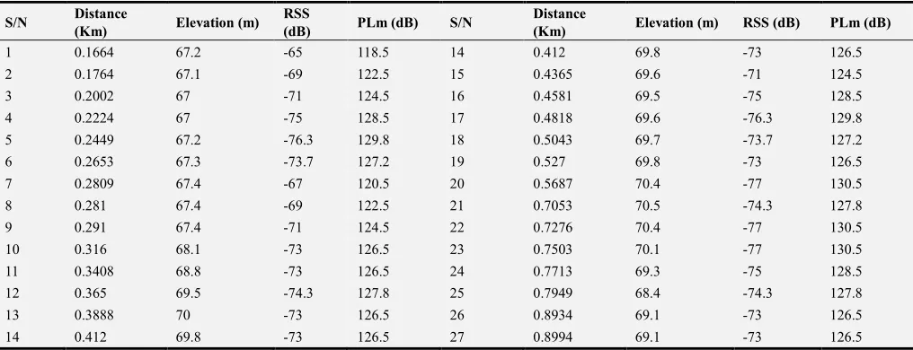
The field measured distance, elevation, received signal strength (RSSI) and pathloss (PLm) are given in Table 1. The measured pathloss (PLm) is obtained by using the link budget equation;
+,-(./) = 53.5 (dBm). – RSS (dBm). The distance is
obtained by applying the longitude and latitude of each of the measurement points in the Haversine equation with the longitude 1 and latitude 1 being that of the GSM base station while longitude 2 and latitude 2 is for each of the measurement points.
Figure 1. The Elevation Profile of the terrain.
Table 1. The Field Measured Distance, Elevation, Received Signal Strength (RSS) and Pathloss (PLm).
S/N Distance
(Km) Elevation (m)
RSS
(dB) PLm (dB) S/N
Distance
(Km) Elevation (m) RSS (dB) PLm (dB)
1 0.1664 67.2 -65 118.5 14 0.412 69.8 -73 126.5
2 0.1764 67.1 -69 122.5 15 0.4365 69.6 -71 124.5
3 0.2002 67 -71 124.5 16 0.4581 69.5 -75 128.5
4 0.2224 67 -75 128.5 17 0.4818 69.6 -76.3 129.8
5 0.2449 67.2 -76.3 129.8 18 0.5043 69.7 -73.7 127.2
6 0.2653 67.3 -73.7 127.2 19 0.527 69.8 -73 126.5
7 0.2809 67.4 -67 120.5 20 0.5687 70.4 -77 130.5
8 0.281 67.4 -69 122.5 21 0.7053 70.5 -74.3 127.8
9 0.291 67.4 -71 124.5 22 0.7276 70.4 -77 130.5
10 0.316 68.1 -73 126.5 23 0.7503 70.1 -77 130.5
11 0.3408 68.8 -73 126.5 24 0.7713 69.3 -75 128.5
12 0.365 69.5 -74.3 127.8 25 0.7949 68.4 -74.3 127.8
13 0.3888 70 -73 126.5 26 0.8934 69.1 -73 126.5
Table 2. The Elevation, The Mean Elevation and The Standard Deviation Of The Elevation.
S/N Elevation (m) S/N Elevation (m) S/N altitude (m)
1 67.2 10 68.1 19 69.8 Mean Elevation (Ē)
2 67.1 11 68.8 20 70.4 68.76667
3 67 12 69.5 21 70.5
4 67 13 70 22 70.4 Standard Deviation (•)
5 67.2 14 69.8 23 70.1 1.215334
6 67.3 15 69.6 24 69.3
7 67.4 16 69.5 25 68.4
8 67.4 17 69.6 26 69.1
9 67.4 18 69.7 27 69.1
Table 2 shows the elevation, the mean elevation and the standard deviation of the elevation of the measurement points. The Hata model will be optimised using the mean elevation and then using the standard deviation of the elevation of the measurement points.
Microsoft Excel solver is used to determine the value of
Kjand also the value of KŠ that minimizes the sum of square error. The results obtained from the Microsoft Excel solver are
Kj= 0.641859 and KŠ = 36.31799. Therefore, with mean
elevation (Mj) =68.76667, Kj = 0.641859, hence;
Cj = Kj(Mj) = 44.13848.
Also, with standard deviation of elevation (Š) = 1.215334,
KŠ = 36.31799, hence;
CŠ = KŠ (Š) = 44.13848
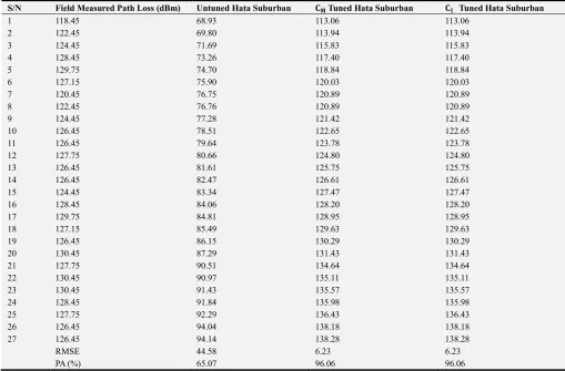
Table 3 shows the field measure pathloss and the pathloss predicted by the untuned Hata model, the pathloss predicted by the mean elevation tuned Hata model and the pathloss predicted by the standard deviation of elevation tuned Hata model. Also, the table shows that the untuned Hata model has a RMSE of 44.58 dB and prediction accuracy of 65.07%. On the other hand, both the pathloss predicted by the mean elevation tuned Hata model and the pathloss predicted by the standard deviation of elevation tuned Hata model have the same RME of of 6.23 dB and prediction accuracy of 96.06%. The correction factors are the same value (that is, CŠ = Cj =
44.13848). Finally, with the RMSE about 6 dB, it can be concluded that the terrain parameter-based tuning approach can effectively be used to minimize the prediction error of the Hata model within the acceptable value which is about 7dB to 10 dB for urban and rural areas.
Table 3. The field measure pathloss and the pathloss predicted by the untuned and the tuned Hata model.
S/N Field Measured Path Loss (dBm) Untuned Hata Suburban •‘jTuned Hata Suburban •Š Tuned Hata Suburban
1 118.45 68.93 113.06 113.06
2 122.45 69.80 113.94 113.94
3 124.45 71.69 115.83 115.83
4 128.45 73.26 117.40 117.40
5 129.75 74.70 118.84 118.84
6 127.15 75.90 120.03 120.03
7 120.45 76.75 120.89 120.89
8 122.45 76.76 120.89 120.89
9 124.45 77.28 121.42 121.42
10 126.45 78.51 122.65 122.65
11 126.45 79.64 123.78 123.78
12 127.75 80.66 124.80 124.80
13 126.45 81.61 125.75 125.75
14 126.45 82.47 126.61 126.61
15 124.45 83.34 127.47 127.47
16 128.45 84.06 128.20 128.20
17 129.75 84.81 128.95 128.95
18 127.15 85.49 129.63 129.63
19 126.45 86.15 130.29 130.29
20 130.45 87.29 131.43 131.43
21 127.75 90.51 134.64 134.64
22 130.45 90.97 135.11 135.11
23 130.45 91.43 135.57 135.57
24 128.45 91.84 135.98 135.98
25 127.75 92.29 136.43 136.43
26 126.45 94.04 138.18 138.18
27 126.45 94.14 138.28 138.28
RMSE 44.58 6.23 6.23
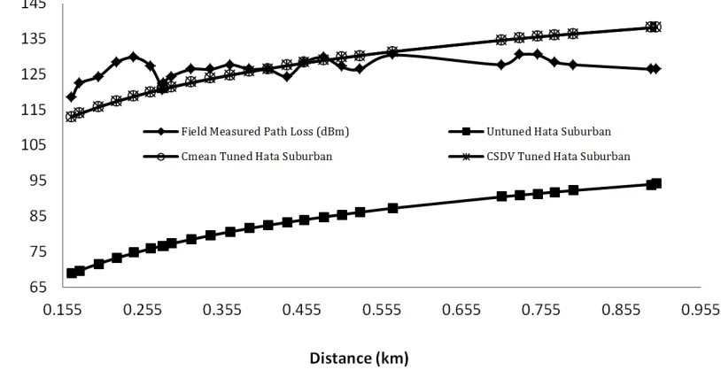
Figure 2. The field measure pathloss and the pathloss predicted by the untuned and the tuned Hata models.
4. Conclusion
In this paper, terrain roughness parameter-based tuning approach is presented for Hata model. The study is based on empirical field measurement in a suburban area for a GSM network in the 800 MHz frequency band. In most published works, the standard deviation of the elevation is used to characterize the terrain roughness. However, the mean elevation and the standard deviation of elevation are used separately in this paper to minimize the error using least square method. The results show that the two approach gave the same correction factor for Hata propagation model and hence, the same RMSE and prediction accuracy. Also, both approach reduced the Hata model prediction error within the acceptable 7 dB for suburban and rural areas.
References
[1] Ranvier, S. (2004). Path loss models. Helsinki University of Technology.
[2] Roslee, M. B., & Kwan, K. F. (2010). Optimization of Hata propagation prediction model in suburban area in Malaysia. Progress In Electromagnetics Research C, 13, 91-106. [3] Singh, Y. (2012). Comparison of Okumura, Hata and
COST-231 Models on the Basis of Path Loss and Signal Strength. International Journal of Computer Applications, 59 (11).
[4] Randeep S. C., Yuvraj S., Sandeep S. and Rakesh G., (2015) Performance & Evaluation of Propagation Models for Sub-Urban Areas. International Journal of Advanced Research in Electrical, Electronics and Instrumentation Engineering. Vol. 4, Issue 2, February 2015.
[5] Nadir, Z., Elfadhil, N., & Touati, F. (2008, July). Pathloss determination using Okumura-Hata model and spline interpolation for missing data for Oman. In Proceedings of the world congress on Engineering (Vol. 1, pp. 2-4).
[6] Abhayawardhana, V. S., Wassell, I. J., Crosby, D., Sellars, M. P., & Brown, M. G. (2005, May). Comparison of empirical propagation path loss models for fixed wireless access systems. In 2005 IEEE 61st Vehicular Technology Conference (Vol. 1, pp. 73-77). IEEE.
[7] Alumona, T. L. (2015). Path Loss Prediction of Wireless Mobile Communication for Urban Areas of Imo State, South-East Region of Nigeria at 910 MHz. International Journal of Sensor Networks and Data Communications, 2015. [8] Thomas, T., & Vivek, M. V. (2015). Path loss Determination
Using Hata Model and Effect of Path loss in OFDM. environment, 1 (8).
[9] Ekka, A. (2012). Pathloss Determination Using Okumura-hata Model for Rourkela (Doctoral dissertation, National Institute of Technology Rourkela).
[10] Verma, R., & Saini, G. (2015). DIFFERENT PROPAGATION MODELLING TOOLS USED FOR VARIOUS INDOOR AND OUTDOOR SCENARIOS.
[11] Phillips, C., Sicker, D., & Grunwald, D. (2012). Bounding the practical error of path loss models. International Journal of Antennas and Propagation, 2012.
[12] Bhuvaneshwari, A., Hemalatha, R., & Satyasavithri, T. (2013, October). Statistical tuning of the best suited prediction model for measurements made in Hyderabad city of Southern India. In Proceedings of the world congress on engineering and computer science (Vol. 2, pp. 23-25).
[13] Keawbunsong, P., Supannakoon, P., & Promwong, S. (2015). Optimized Walficsh-Bertoni Model for Path Loss Prediction DTTV Propagation in Urban Area of Southern Thailand. Advanced Science Letters, 21 (10), 3029-3032.
[14] Keawbunsong, P., Supannakoon, P., & Promwong, S. (2015). Optimization of Path Loss Model for Prediction DTTV Propagation in Urban Area of Southern Thailand. Advanced Science Letters, 21 (10), 3064-3068.
[16] Mousa, A., Dama, Y., Najjar, M., & Alsayeh, B. (2012). Optimizing Outdoor Propagation Model based on Measurements for Multiple RF Cell. International Journal of Computer Applications, 60 (5).