R E S E A R C H
Open Access
Compensation of feature selection biases
accompanied with improved predictive
performance for binary classification by using
a novel ensemble feature selection approach
Ursula Neumann
1,2,3, Mona Riemenschneider
1,2, Jan-Peter Sowa
4, Theodor Baars
5, Julia Kälsch
4,
Ali Canbay
4and Dominik Heider
1,2,3**Correspondence: [email protected] 1Department of Bioinformatics, 94315, Straubing, Germany 3Wissenschaftszentrum Weihenstephan, Technische Universität München, 85354, Freising, Germany
Full list of author information is available at the end of the article
Abstract
Motivation: Biomarker discovery methods are essential to identify a minimal subset of features (e.g., serum markers in predictive medicine) that are relevant to develop prediction models with high accuracy. By now, there exist diverse feature selection methods, which either are embedded, combined, or independent of predictive learning algorithms. Many preceding studies showed the defectiveness of single feature selection results, which cause difficulties for professionals in a variety of fields (e.g., medical practitioners) to analyze and interpret the obtained feature subsets. Whereas each of these methods is highly biased, an ensemble feature selection has the advantage to alleviate and compensate for such biases. Concerning the reliability, validity, and reproducibility of these methods, we examined eight different feature selection methods for binary classification datasets and developed an ensemble feature selection system.
Results: By using an ensemble of feature selection methods, a quantification of the importance of the features could be obtained. The prediction models that have been trained on the selected features showed improved prediction performance.
Keywords: Machine learning, Feature selection, Ensemble learning, Biomarker discovery, Random forest
Background
In the fields of predictive medicine as well as molecular diagnostics the need for sim-plification of datasets with many parameters frequently emerges. Therefore, approaches are necessary, which can identify important parameters (sometimes also referred to as features, independent variables, or predictor variables). Such quantifiable parameters that allow diagnostic validity are called biomarkers. In 2001, the Biomarkers Definitions Working Group of the American National Institute of Health defined a biomarker as “a characteristic that is objectively measured and evaluated as an indication of normal biologic processes, pathogenic processes, or pharmacologic responses to a therapeutic intervention“ [1]. Examples for biomarkers are serum parameters, genetic markers, or socio-demographic markers.
The detection of biomarkers can be conducted by computer-assisted approaches, namely feature selection (FS) methods. A great variety of FS techniques already exist. In general, these approaches can be separated into: filter methods, wrapper methods, and embedded methods. The first one is independent of any prediction model and therefore shows an advantage in regards of computation time compared to the other approaches. Filter methods use weighting measures, such as correlation coefficients [2] or mutual information [3]. The wrapper methods are computationally intensive, but in turn pro-vide better accuracy compared to filter methods [4]. This type of approach occurs outside the model construction, however it uses the outcome as a guideline. The third type, the embedded methods, is an alternative to wrapper methods. These approaches combine the advantages of both methods stated above, namely the low computational costs and an adequate accuracy. This is due to the fact that the process of feature selection is already part of the model construction. There are three main criteria a feature selection method should meet, namely reliability, validity, and reproducibility. Methods that display these characteristics are called stable. Based on the definition of biomarkers, non-generalizable features are not considered to be reliable markers. There are several factors that can cause instability of the feature selection, e.g., the complexity of multiple biomarkers, a small-n-large-p-problem, or when the algorithm simply ignores stability [5, 6]. Thus, feature selection results have to be treated with care. For example, the Gini-index is widely used in predictive medicine, but it has also been demonstrated to deliver instable results due to unbalanced datasets [7, 8]. To counteract instability of feature selection methods, we developed an ensemble feature selection (EFS) method, which compensates biases of sin-gle FS. The idea of ensemble methods is already widely used in learning algorithms [9]. In this article we will introduce eight FS methods and our quantifying EFS method. We eval-uated our EFS method compared to the state-of-the-art method AUC-FS with regard to the prediction performance in subsequent classification based on six different datasets. Furthermore, we compared the results with prediction models without pre-selection of features.
Methods
With the development of the EFS method we take advantage of the benefits of multi-ple feature selection methods and combine their normalized outputs to a quantitative ensemble importance. The key features of our EFS method are:
1. The combination of widely known and extensively tested feature selection methods. 2. The balance of biases by using an ensemble.
3. The evaluation of EFS.
Eight different feature selection methods have been used for the EFS approach. Since random forests have drawn increased attention in the field of predictive medicine, four of the chosen feature selection methods are embedded in a random forest algo-rithm. Further, we considered the outcome of a logistic regression (i.e., the coefficients) as another embedded method as well as the filter methods median, Pearson-, and Spearman-correlation.
Y = (y1,. . .,yN)be the response variable. Altogether, a data matrix of sizeN×M+1
is received, where N is the number of samples and M is the number of prediction variables.
Random forest
Random forests (RFs) are ensemble learning methods for classifications and regressions consisting of multiple decision trees [10]. RFs have been shown to give highly accu-rate predictions on biological [11–13] and biomedical data [14, 15]. There are different implementations of the RF algorithm in R available, which offer diverse feature selection methods. In the context of RFs, these feature selection methods are called variable impor-tance measures (VIMs). We integrated two of the available implementations of RFs into our EFS method: (i) the RF method adapted from Breiman [10], which uses the CART (classification and regression tree) algorithm for individual node decisions, implemented in the R package randomForest and (ii) the cforest [16] implementation from the R-packageparty, because of its promising AUC score VIM. In RF approaches, randomness is gained by the general technique of bootstrap aggregating, also called bagging, mean-ing that for the tree buildmean-ing process only a subset of the data samples are chosen with replacement. We used 1000 decision trees in both RFs. In order to get robust results, we averaged the VIMs over 100 RF models.
The raw variable importance score for Xi is given by the average over the set of all
decision treest∈ {1,. . .,T}in the RF:
VIXi=
1
T
T
t=1
VIXi(t).
In addition, we define an indicator functionI(A)by:
I(A)=
1, if the argumentAis fulfilled, 0, otherwise.
Gini-index
The Gini-index is the sum of products between different class proportions over all classes for each variable, which is in the case of a binary classification:
G=2p(1−p), wherep= N1
N is the proportion of one of the classes, in this case for responseY =1, and
N1is the number of units in this class.
The Gini-indexGdefines a measuredijof the decrease in heterogeneity at nodej:
dij=G−(
NL
N GL+ NR
N GR),
whereGRandGLrespectively are the Gini-indexes calculated for the following right and
left nodes andNLandNRare the numbers of units in the left and right node after splitting.
With this measure the variable importance forXiin treetis defined as:
VIXi(t)=
j∈J
dijI(Xisplits at node j).
Mean accuracy error-rate-based VIM
The mean accuracy error-rate-based VIM uses the out-of-bag (OOB) data. The OOB consists of the subset of all samples which are not used for the construction of decision trees: For each tree, the prediction error on the OOB portion of the data is recorded (error rates for classification, mean square errors for regression). This process is repeated after permuting each predictor variable. The difference between both is averaged over all trees, and normalized by the standard deviation of the differences, except the standard deviation is zero. For each treet, we get the following formula:
VIXi(t)=
1
|B(t)|
j∈B(t)
I(yj=pj)−I(yj=pj,πi),
wherepiis the RF prediction of the response variable,πiis the permutation of the values
in thei-th variable andB(t)is the OOB data for treet.
Conditional error-rate-based VIM
In principle, the underlying mathematical model for the conditional error-rate-based VIM is the same as for the mean accuracy error-rate-based VIM. The conditional VIM takes biases in variable importance into account, which are generated by a correlation of the testedXiwith the other prediction variables.
ForZ=X1,. . .,Xi−1,Xi+1,. . .,XMwe calculate
VIXi(t)=
1
|B(t)|
j∈B(t)
I(yj=pj)−I(yj=pj,πi|Z),
whereB(t)is the OOB data for treet. In other words, the variableXiis permuted, whileZ
is fixed atZ =z:=(cp1,. . .,cpi−1,cpi+1,. . .,cpM), consisting of the cut points for each variable inZ, which are defined through the partition of the feature space ofXiinduced
by the current treet.
AUC-based VIM
In contrast to the aforementioned VIMs, the AUC-based VIM does not employ the error-rate, but instead uses the Area Under the Curve (AUC). It is calculated as the integral of the Receiver Operating Characteristic (ROC) curve, which is received by mapping the sensitivity against specificity for every possible cut-off between the two classes.
In contrast to error-rate-based methods, which give more weight to the majority class, the AUC does not favor any class. In previous studies the AUC was shown to be a par-ticularly appropriate VIM for unbalanced data settings and should be considered as the state-of-the-art model [17, 18]. The AUC-score is an estimator for the probability that a randomly chosen sample from classY = 1 receives a higher class probability for class
Y = 1 than a randomly chosen sample from classY = 0. The variable importance for each treetis calculated as:
VIXi(t)=AUCi−AUCπi
whereAUCiandAUCπirespectively are the AUCs computed from the OOB observations
Logistic regression
Even though RFs have become very popular, it is not totally understood why the algo-rithm acts in its specific way. An embedded feature selection method, which is understood in more details, is the weighting system (i.e., coefficients) of the logistic regression. For feature selection, we access the model’s coefficients, i.e., theβ−values of the regression equation. It should be noted that the range of features can strongly differ. Due to this fact, theβ-coefficients of parameters are not directly comparable. To provide comparability of the variables’ importances, we conducted a z-transformation:
zX =
X−X sX
,
whereXis the mean andsX the standard deviation of variableX, respectively. Through
standardization by z-transformation, the mean of β-coefficients become zero with a standard deviation of 1, thus assuring that the features all have the same domain. Subsequently, the values are ordered according to their absolute values in decreasing order.
Correlation coefficient
The correlation between any two features can be described as the quantification of the extent of statistical dependence between them, which can be quantified by different cor-relation coefficients. We used the approach of [19] to select features that are highly correlated with the dependent variable, but show only low correlation with other predic-tors. We used a threshold for the correlation between the predictor variables ofp= 0.7. In order to avoid collinearity a threshold of 0.7 is most frequently used [20], although recommendations for more restrictive (e.g., 0.4 [21]) and less restrictive (e.g., 0.8 [22]) thresholds exist. In our study, we adopted two correlation coefficients, namely the Pearson product-moment correlation and the Spearman rank correlation coefficient.
Pearson
For any two featuresXandY with samplesj = 1,. . .,n, the Pearson product-moment correlation coefficient is defined as
rXY =
n
j=1(xj−x)(yj−y)
n
j=1(xj−x)2nj=1(yj−y)2
,
wherexandyare the sample means ofXandY.
Spearman
For the Spearman rank correlation coefficient we observe the sample’s ranksrk(xi)and
rk(yi)of the featuresX=(x1,. . .,xn)andY=(y1. . .,yn)and compute
ρ=1−6
n
j=1
d2i n(n2−1),
Median
For the median feature selection, we used a Mann-Whitney-U test [23] comparing the positive and negative class of the response variableY. The test evaluates following hypoth-esis: Sincemed0andmed1are the medians of the negative and positive class of a predictor
variable, the null hypothesis for each predictor variable is defined as:
H0:med0=med1.
The resulting p-values of the Mann-Whitney-U test are used as scoring system for the feature selection. Thus, a smaller p-value indicates a higher importance.
Ensemble feature selection
Feature selection methods as a preprocessing step for supervised learning algorithms provide several benefits, such as reduced computational costs (e.g., training time, stor-age requirements), but also improved prediction performance. However, different feature selection methods provide different subsets of features. Hence they give rise to sample selection bias. In general, the aim of supervised learning algorithms is to find a suitable hypothesis which makes the best prediction for a particular problem. Improvements can be achieved by combining multiple hypotheses instead of testing only one. This is the main concept of ensemble learning methods. Ensemble techniques are widely used in machine learning algorithms to achieve higher stability. The RF algorithm is an example for bootstrap aggregating [24]. This technique combines several prediction models using a randomly drawn subset of the training data. Another type of ensemble learning meth-ods are boosting algorithms, which merge several weak classifiers to a stronger one. The most popular implementation is AdaBoost [25].
In the current study, we developed a stable feature selection procedure, which is based on the idea of ensemble learning. For our EFS method we integrated eight different feature selection methods and normalized all individual outputs to a common scale, an interval from 0 to 1. Thereby we ensure the comparability between different FS methods and con-serve the distances of importance between one feature to another. This normalization is achieved in two different ways: For all feature selections, except for the median, the abso-lute value of the FS method output is a value which illustrates the increase of importance. By dividing through the maximum value we get values between 1 and 0:
impXi= βi
max(βm)m∈M
.
In the case of the median FS we receive a p-value for each feature Xi, which is
normalized as follows:
impXi=1−pi+min(pi).
For the four RF based VIMs, we computed 100 repetitions and averaged the importance for each feature. This procedure guarantees a higher robustness of the feature importance and the selected subset.
different methodologies. The EFS system selects those parameter that have a higher importance than the mean importance:
impXi>impXM,
whereimpXMsymbolizes the mean of all variable importances. Alternatively, the median
or Q3 could be used as well, however, both would lead to a fixed number of selected parameter irrespective of their relevance for the subsequent classification model.
The logistic regression model based on the EFS-selected features was then compared to logistic regression models either trained on all features and on features selected by the AUC-based VIM, which is considered to be one of the state-of-the-art methods for feature selection. We examined the AUC-values of the ROC curves with ROCR [27]. Additionally, the improvement in performance between the AUC-based VIM, the EFS subset, and the model without feature selection is measured by a comparison of the AUCs via the method of DeLong et al. [28].
Datasets
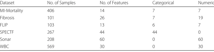
To evaluate our EFS method, we used six different datasets. An overview of the datasets is given in Table 1.
The first datasetMI-Mortalitywas provided by the Clinic for Cardiology, West German Heart and Vascular Centre Essen of the University Hospital Duisburg-Essen. It con-sists of 14 socio-demographic and serum parameters from 406 patients. The purpose of this study was to examine which parameters are important for the mortality predic-tion after treatment on myocardial infarcpredic-tion. The data was collected during a follow-up study of [29].
The Department of Gastroenterology and Hepatology of the University Hospital Duisburg-Essen provided the datasets Fibrosis [30] and FLIP, which again consist of socio-demographic and serum parameters. Both deal with different scores to predict fibrosis.
SPECTFis a dataset from the UCI Machine Learning Repository [31]. It describes diag-nosing of cardiac Single Proton Emission Computed Tomography (SPECT) images. The class-variable is distinguishing between normal (=0) and abnormal (=1).
TheSonardataset has also been retrieved from the UCI Machine Learning Repository and obtained by bouncing sonar signals off a metal cylinder or rock at various angles and under various conditions. The prediction model should be able to distinguish between rocks and metal cylinders.
In theWBCdataset a classification between benign and malignant tumors in breast cancer samples is intended. Benign tumors are not cancerous, thus these samples are class 0. Malignant tumor samples are class 1.
Table 1Overview of datasets. Number of features after removing samples with missing values
Dataset No. of Samples No. of Features Categorical Numeric
MI-Mortality 406 14 7 7
Fibrosis 101 26 7 19
FLIP 103 13 6 7
SPECTF 267 44 44 0
Sonar 208 60 0 60
In order to reduce the number of missing values in the datasets, features with more than 20% missing values were discarded. Additionally, columns with zero variance were removed.
Results
Selected features
The number of selected features from EFS and AUC-FS varies for each dataset. The Gini FS method is known to prefer categorical variables with many categories and disregards potential important binary prediction variables [32]. In contrast to the Gini FS, we could observe that the variable type did not play a decisive role for the importance. Through aggregating different FS methods into an ensemble, biases of individual methods are compensated.
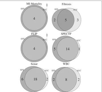
In Fig. 1 Venn diagrams are shown, illustrating the feature subsets derived from the AUC-FS and EFS, respectively. The Venn diagrams show no distinct trend for the number of features that were selected by the respective method, i.e., in some datasets EFS selects more features than the AUC-FS, while in other datasets it is the other way around.
For theFibrosisdata the selected subset of AUC-FS contains eight features, whereas the EFS subset consists of only seven. Five features have been selected by both methods, while the other features are disjoint. TheWBCdataset yielded a similar result. Both methods selected a subset of ten features, with eight features being selected by both methods. The
results of theMI-Mortalitydata andFLIPdata are similar: EFS selected a subset of five features while AUC-FS returned four features, which all are contained in the EFS selected subset. The datasets of the SPECTF resp. Sonarstudies also deliver analogous subset schemes. The major part of selected features are chosen by both FS methods (14 and 18, respectively). Our EFS method considered five and six additional features, while the AUC-FS selected one and two additional features, which do not occur in the intersection of both subsets.
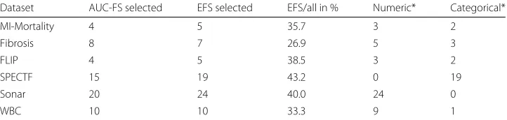
The EFS selected more features than the AUC-FS in four out of six cases, however the percentages of selected features out of all possible prediction variables ranged from 26.9 to 43.2% (cf. Table 2).
Performance evaluation
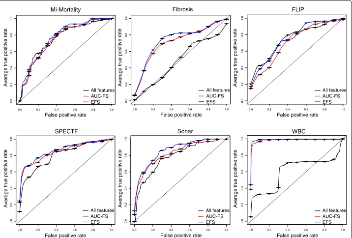
In order to evaluate our EFS method in comparison to the AUC-FS, we used a logistic regression model with LOOCV. Additionally, we trained a logistic regression model with-out feature selection. Table 3 summarizes the results for all datasets. The resulting ROC curves are shown in Fig. 2.
For each dataset, the resulting model trained on the EFS selected subset of features per-formed superior compared to the models trained either on the AUC-FS selected features or on all features without selection.
However, the EFS showed a significantly higher AUC value only for the dataset WBC. For all other datasets, the AUCs were higher for the EFS compared to the AUC-FS as well, however the results were not significant: MI-Mortality (p=0.228), Fibrosis (p=0.273), FLIP (p=0.254), SPECTF (p=0.444), Sonar (p=0.2), and WBC (p=0.02).
The model using the EFS selected features showed significant higher AUC values com-pared to the model trained without feature selection for all datasets except MI-Mortality and FLIP (p=0.201 andp=0.971, respectively). Taken together, throughout all datasets we can observe an enhancement of performance by using the EFS method, although it is not significant in all datasets.
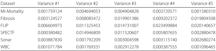
Additionally, we evaluated the robustness of our EFS approach by using permutation tests [33, 34]. To this end, the logistic regression models are compared to models that are trained on randomly permuted class labels. P-values for all datasets were less than 0.001. Moreover, we evaluated the stability of the EFS approach in terms of selected features. To this end, we evaluated the variance of the importance of the five most important fea-tures using a 10-fold cross-validation of the datasets repeated 10 times. Furthermore, we used the Jaccard-index [35] as a stability score, described by the following formula:
J(S1,. . .,Sn)= |
S1∩. . .∩Sn|
|S1∪. . .∪Sn|
,
Table 2Types of selected features. Evaluation of the selected features subsets of AUC-FS and EFS
Dataset AUC-FS selected EFS selected EFS/all in % Numeric* Categorical*
MI-Mortality 4 5 35.7 3 2
Fibrosis 8 7 26.9 5 3
FLIP 4 5 38.5 3 2
SPECTF 15 19 43.2 0 19
Sonar 20 24 40.0 24 0
WBC 10 10 33.3 9 1
Table 3Results on datasets
Dataset All [CI] AUC-FS [CI] EFS [CI] AUC-FS vs. EFS* all vs. EFS** MI-Mortality 0.758 [0.700, 0.800] 0.757 [0.704, 0.811] 0.776 [0.725, 0.826] 0.228 0.201 Fibrosis 0.493 [0.300, 0.600] 0.681 [0.537, 0.824] 0.746 [0.617, 0.874] 0.273 0.018
FLIP 0.759 [0.600, 0.900] 0.723 [0.582, 0.863] 0.761 [0.633, 0.890] 0.254 0.971 SPECTF 0.807 [0.700, 0.900] 0.856 [0.811, 0.901] 0.865 [0.821, 0.910] 0.444 4.68e-4 Sonar 0.792 [0.700, 0.900] 0.840 [0.787, 0.894] 0.862 [0.813, 0.911] 0.200 0.009
WBC 0.611 [0.600, 0.700] 0.987 [0.977, 0.998] 0.991 [0.981, 1.000] 0.020 1.21e-41
Column 1 to 3 are AUCs values of all features, selected by AUC-FS and by the EFS with confidential intervalls in brackets. The last two columns show thep-values of the comparison by the method of [28]. The function compares the AUC of the ROC curves of (*) the AUC-FS and EFS method and (**) of all parameters and EFS outcome. Statistical significantp-values are printed in bold
whereS1,. . .,Snare different subsets of features. Thereby, a Jaccard-index close to 1
rep-resents a high similarity of feature subsets. It turned out that EFS gives highly stable results with variances of the importance values less than 0.0235. Moreover, the Jaccard-index of the selected features by EFS was 1 for all data sets. Table 4 shows all variances of the importance and the corresponding boxplots can be found in the Additional file 1.
Discussion
Feature selection methods have been studied for several decades (e.g., [36]). There are already many publications [37–41] on how to improve the performance of feature selection methods.
We provide an ensemble feature selection tool to conduct a feature selection for binary classification, which showed promising performance on all datasets. In contrast to ensem-ble methods of previous studies [42–44], the aim of this work was to combine filter
Mi-Mortality Fibrosis FLIP
False positive rate False positive rate False positive rate
False positive rate False positive rate False positive rate
Average true positive rate
et ar e viti s o p e urt e g ar e v A et ar e vit is o p e urt e g ar e v A
Average true positive rate
et ar e vit i s o p e urt e g ar e v A et ar e vit i s o p e urt e g ar e v A
0.0 0.2 0.4 0.6 0.8 1.0
0.0 0.2 0.4 0.6 0.8 1.0
0.0 0.2 0.4 0.6 0.8 1.0
0.0 0.2 0.4 0.6 0.8 1.0
0.0 0.2 0.4 0.6 0.8 1.0
0.0 0 .2 0.4 0 .6 0.8 1 .0
0.0 0.2 0.4 0.6 0.8 1.0
0.0 0.2 0.4 0.6 0.8 1.0
0.0 0.2 0.4 0.6 0.8 1.0
0.0 0 .2 0.4 0 .6 0.8 1 .0
0.0 0.2 0.4 0.6 0.8 1.0
0.0 0.2 0.4 0.6 0.8 1.0
SPECTF Sonar WBC
All features AUC-FS EFS All features AUC-FS EFS All features AUC-FS EFS All features AUC-FS EFS All features AUC-FS EFS All features AUC-FS EFS
Table 4Variance of feature importances. Variance of the five most important features of a 10-fold cross-validation
Dataset Variance #1 Variance #2 Variance #3 Variance #4 Variance #5 MI-Mortality 0.001759124 0.004694053 0.004904828 0.003720571 0.001580310 Fibrosis 0.003124527 0.008085472 0.019901386 0.009202372 0.019804508 FLIP 0.006604973 0.011325453 0.014731007 0.023499884 0.020140657 SPECTF 0.000380482 0.014946809 0.011520607 0.005807655 0.002880478 Sonar 0.003887830 0.001792209 0.003004598 0.003115140 0.002680274 WBC 0.001071784 0.001769331 0.002912278 0.000387555 0.001096465
and embedded methods. Due to their focus on predictions, embedded methods usu-ally attain a higher prediction performance, whereas the advantage of filter methods are low computational cost and low complexity. By using ensembles, the advantages of both strategies can be combined and individual biases are alleviated. Concerning the enhanced approximation of embedded methods, we excluded wrapper methods from our study.
The cforest method requires more time than any other component of the EFS algorithm, thus calculations of datasets with hundreds of thousands of features would take up a lot of CPU time. A workload saving alternative would be a reduction of the repetition rate of the RF algorithms, in particular of the cforest algorithms. However, in turn this will negatively affect the VIM’s robustness. In our computations the repetition rate was set to 100 and the average variable importance was reported. Since, there is no generalization on how many repeats are necessary to get a robust result.
The evaluation of feature subsets depicted in the Venn diagrams reflects that in four out of six cases our EFS method selects more features than the AUC-FS. We assume that the reason for this phenomenon is based on the importance weighting system of the AUC-FS. As threshold for the decision which features are considered to be the most important ones, the respective mean over all importance values was taken. If there are only a few features lying above average, this might be an indication that the values of those features which are considered important are overestimated compared to the non-selected fea-tures. Thus the mean increases and less features reach that threshold. Alternatively, the opposite case could be true, meaning in one or more of the other feature selection meth-ods the assigned importance values hardly differ. This in turn has an alleviating factor on the importance values of our ensemble of feature selection methods.
In the current study, we used the logistic regression method to analyze the perfor-mance of our EFS. For binary classification, logistic regression is the statistical method of choice, in particular in the field of predictive medicine [45]. It has the ability of detecting possible causal relationships between features. By conducting a z-transformation on the whole dataset the relationships become easy to interpret via theβ-coefficients. Although the logistic regression model has many advantages, the prediction performance could be improved by using other predictive models in future studies. To get a broader and more generalizable rating for the results of our EFS method, an evaluation by methods such as support vector machines or RFs could additionally be conducted.
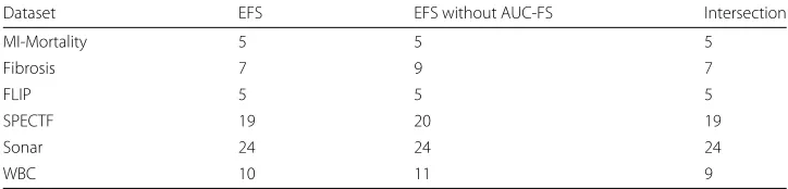
Table 5Quantity of selected features. Number of selected features of our EFS method with and without the AUC-FS
Dataset EFS EFS without AUC-FS Intersection
MI-Mortality 5 5 5
Fibrosis 7 9 7
FLIP 5 5 5
SPECTF 19 20 19
Sonar 24 24 24
WBC 10 11 9
importance of features. This issue could be solved by a weighted majority vote. For more details on fusion methods we refer to [9].
We determined several thresholds for the computation, namely the number of repe-titions of the RF algorithms (100 times), the threshold of missing values (20%), and the correlation threshold between the dependent variables (0.7). In some data cases varying these thresholds might yield a better performance. However, for comparability reasons we used fixed thresholds for all datasets.
We also examined the subsets of features selected by the EFS method without the AUC-FS to estimate the influence of the AUC-AUC-FS. The selected features are essentially the same (cf. Table 5). In three datasets the subsets are slightly larger, which supports our theory on the overestimating effect of the AUC-FS on relevant feature’s importance.
By the stability-test we proofed, that the EFS method is a stable and reliable approach for binary classification.
Conclusion
In the current study, we could show the advantages of our EFS method for binary classi-fication data, namely the robustness and stability of feature ranking and subset selection. The evaluation of prediction performance via ROC curves of a logistic regression model showed an improvement of the prediction based on the EFS selected features compared to all features on every tested dataset.
Further investigations on the topic of enhancing feature selection methods will be con-ducted in future. Firstly, we will evaluate our EFS method on high-dimensional data, such as data retrieved from microarray or next-generation sequencing analyses. So far we used datasets with less than 600 samples and a maximum of 60 features. Secondly, in future studies we would like to investigate how our method deals with multiple classes instead of binary classification. Therefore, it will be necessary to substitute the median feature selec-tion method with an appropriate alternative. Another interesting applicaselec-tion will be the extension on regression models where classes are replaced by continuous values. Another direction of our future work on EFS methods will concern the composition of our FS method set. By combining feature selection algorithms the accuracy will improve by the expense of increased complexity. Using an ensemble of several simple methods can gain a higher accuracy than one complex method (cf. [9]). Due to this theory, an evaluation is needed on which FS methods are mandatory to gain a maximum accuracy.
Additional file
Abbrevations
AUC: Area under the curve; CART: Classification and regression tree; CPU: Central processing unit; EFS: Ensemble feature selection; FS: Feature selection; LOOCV: Leave-one-out cross validation; OOB: Out-of-bag; RF: Random forest; ROC: Receiver operating characteristic; VIM: Variable importance measure
Acknowledgements
We are grateful to the UCI Machine Learning Repository for granting access to a great variety of datasets.
Funding
This work was supported by the Deichmann Foundation, which had no role in study design, collection, analysis, and interpretation of data, and in writing the manuscript. This work was supported by the German Research Foundation (DFG) and the Technische Universität München within the funding programme Open Access Publishing.
Availability of data and material
The datasetsSPECTF, SonarandWBCin this article are available in the UCI Machines Learning repository, http://archive.ics. uci.edu/ml. Other datasets of this study are available from University Hospital Duisburg-Essen but restrictions apply to the availability of these data, which were used under license for the current study, and so are not publicly available. Data are however available from the authors upon reasonable request and with permission of University Hospital Duisburg-Essen.
Author’ contributions
UN developed the EFS framework and performed data analyses. JPS, TB, JK, and AC participated in designing the evaluation and in selecting the medical datasets. UN, MR, and DH wrote the manuscript. DH supervised the study. All authors read and approved the final manuscript.
Competing interests
The authors declare that they have no competing interests.
Consent for publication Not applicable.
Ethics approval and consent to participate Not applicable.
Author details
1Department of Bioinformatics, 94315, Straubing, Germany.2University of Applied Science, Weihenstephan-Triesdorf, 85354, Freising, Germany.3Wissenschaftszentrum Weihenstephan, Technische Universität München, 85354, Freising, Germany.4Department of Gastroenterology and Hepatology, University Hospital, University Duisburg-Essen, 45122, Essen, Germany.5Clinic for Cardiology, West German Heart and Vascular Centre Essen, University Hospital, University Duisburg-Essen, 45122, Essen, Germany.
Received: 23 June 2016 Accepted: 27 October 2016
References
1. Biomarkers Definitions Working Group. Biomarkers and surrogate endpoints: preferred definitions and conceptual framework. Clin Pharmacol Therap. 2001;69(3):89–95.
2. Hall M. Correlation-based feature selection for machine learning. 1999. PhD thesis, Department of Computer Science, Waikato University, New Zealand.
3. Peng H, Long F, Ding C. Feature selection based on mutual information: Criteria of max-dependency, max-relevance, and min-redundancy. IEEE Trans Pattern Anal Mach Intell. 2005;27(8):1226–38. 4. Kohavi R, John GH. Wrappers for feature subset selection. Artif Intell. 1997;97:273–324.
5. Jain A, Zongker D. Feature selection: evaluation, application, and small sample performance. IEEE Trans Pattern Anal Mach Intell. 1997;19(2):153–8.
6. He Z, Yu W. Stable feature selection for biomarker discovery. Comput Biol Chem. 2010;34:215–25.
7. Sandri M, Zuccolotto P. A bias correction algorithm for the gini variable importance measure in classification trees. J Comput Graph Stat. 2008;17(3):611–28.
8. Boulesteix AL, Janitza S, Kruppa J, KÃ ˝unig IR. Overview of random forest methodology and practical guidance with emphasis on computational biology and bioinformatics. Wiley Interdisciplinary Rev Data Mining Knowl Discov. 2012;2(6):493–507.
9. Kuncheva LI. Combining Pattern Classifiers: Methods and Algorithms. Hoboken: John Wiley & Sons; 2004. 10. Breiman L. Random forests. Mach Learn. 2001;45(1):5–32.
11. Heider D, Hauke S, Pyka M, Kessler D. Insights into the classification of small gtpases. Adv Appl Bioinform Chem. 2010;3:15–24.
12. van den Boom J, Heider D, Martin SR, Pastore A, Mueller JW. 3-phosphoadenosine 5-phosphosulfate (paps) synthases, naturally fragile enzymes specifically stabilized by nucleotide binding. J Biol Chem. 2012;287(21): 17645–55.
13. Touw WG, Bayjanov JR, Overmars L, Backus L, Boekhorst J, Wels M, van Hijum SA. Data mining in the life sciences with random forest: a walk in the park or lost in the jungle? Brief Bioinform. 2013;14(3):315–26.
15. Riemenschneider M, Senge R, Neumann U, Hüllermeier E, Heider D. Exploiting hiv-1 protease and reverse transcriptase cross-resistance information for improved drug resistance prediction by means of multi-label classification. BioData Mining. 2016;9:10.
16. Hothorn T, Hornik K, Zeileis A. Party: A Laboratory for Recursive Part(y)itioning. http://CRAN.R-project.org/. 17. Calle M, Urrea V, Boulesteix LA, Malats N. Auc-rf: A new strategy for genomic profiling with random forest. Hum
Heredity. 2011;72(2):121–32.
18. Janitza S, Strobl C, Boulesteix AL. An auc-based permutation variable importance measure for random forests. BMC Bioinformatics. 2013;14:119.
19. Yu L, Liu H. Efficient feature selection via analysis of relevance and redundancy. J Mach Learn Res. 2004;5:1205–24. 20. Dormann CF, Elith J, Bacher S, Buchmann C, Carl G, Carr G, Marquz JRG, Gruber B, Lafourcade B, Leito PJ,
Mnkemller T, McClean C, Osborne PE, Reineking B, Schrder B, Skidmore AK, Zurell D, Lautenbach S. Collinearity: a review of methods to deal with it and a simulation study evaluating their performance. Ecography. 2013;36(1):27–46. 21. Suzuki N, Olson DH, Reilly EC. Developing landscape habitat models for rare amphibians with small geographic
ranges: a case study of siskiyou mountains salamanders in the western usa. Biodiversity Conserv. 2008;17:2197–218. 22. Elith J, Graham CH, Anderson RP, Dudk M, Ferrier S, Guisan A, Hijmans RJ, Huettmann F, Leathwick JR, Lehmann A, Li J, Lohmann LG, Loiselle BA, Manion G, Moritz C, Nakamura M, Nakazawa Y, Overton JM, Townsend Peterson A, Phillips SJ, Richardson K, Scachetti-Pereira R, Schapire RE, Sobern J, Williams S, Wisz MS, Zimmermann NE. Novel methods improve prediction of species distributions from occurrence data. Ecography. 2006;29(2):129–51. 23. Bauer DF. Constructing confidence sets using rank statistics. J Am Stat Assoc. 1972;67:687–90.
24. Breiman L. Bagging predictors. Mach Learn. 1996;24(2):123–40.
25. Freund Y, Schapire RE. A decision-theoretic generalization of on-line learning and an application to boosting. J Comput Syst Sci. 1997;55(1):119–39.
26. Hastie T, Tibshirani R, Friedman J. The Elements of Statistical Learning: Data Mining, Inference, and Prediction. New York: Springer; 2011.
27. Sing T, Sander O, Beerenwinkel N, Lengauer T. Rocr: visualizing classifier performance in r. Bioinformatics. 2005;21(20):3940–1.
28. DeLong ER, DeLong DM, Clarke-Pearson DL. Comparing the areas under two or more correlated receiver operating characteristic curves: A nonparametric approach. Biometrics. 1988;44(3):837–45.
29. Baars T, Neumann U, Jinawy M, Hendricks S, Sowa JP, Klsch J, Riemenschneider M, Gerken G, Erbel R, Heider D, Canbay A. In acute myocardial infarction liver parameters are associated with stenosis diameter. Medicine. 2016;95(6):2807.
30. Sowa JP, Heider D, Bechmann LP, Gerken G, Hoffmann D, Canbay A. Novel algorithm for non-invasive assessment of fibrosis in nafld. PLOS ONE. 2013;8(4):62439.
31. Lichman M. UCI Machine Learning Repository. 2013. http://archive.ics.uci.edu/ml.
32. Strobl C, Boulesteix AL, Zeileis A, Hothorn T. Bias in random forest variable importance measures: Illustrations, sources and a solution. BMC Bioinformatics. 2007;8(25):1–21.
33. Barbosa E, Rttger R, Hauschild AC, Azevedo V, Baumbach J. On the limits of computational functional genomics for bacterial lifestyle prediction. Brief Funct Genomics. 2014;13:398–408.
34. Sowa JP, Atmaca, Kahraman A, Schlattjan M, Lindner M, Sydor S, Scherbaum N, Lackner K, Gerken G, Heider D, Arteel GE, Erim Y, Canbay A. Non-invasive separation of alcoholic and non-alcoholic liver disease with predictive modeling. PLOS ONE. 2014;9(7):101444.
35. Kalousis A, Prados J, Hilario M. Stability of feature selection algorithms: a study on high-dimensional spaces. Knowl Inform Syst. 2007;12:95–116.
36. Mucciardi AN, Gose EE. A comparison of seven techniques for choosing subsets of pattern recognition properties. IEEE Trans Comput. 1971;9:1971910231031.
37. Almuallim H, Dietterich TG. Learning with many irrelevant features. 1991547–552. Proceedings of the Ninth National Conference on Artificial Intelligence,San Jose, CA: AAAI Press.
38. Doak J. An evaluation of feature-selection methods and their application to computer security (technical report cse-92-18). Davis: University California, Department of Computer Science. 1992.
39. Caruana RA, Freitag D. Greedy attribute selection. In: Proceedings of the Eleventh Inter-national Conference on Machine Learning. New Brunswick, NJ: Morgan Kaufmann; 1994. p. 28–36.
40. Kononenko I. On biases in estimating multi-valued attributes. Montreal; 1995. p. 1034–1040.
41. Blum AL, Langleyb P. Selection of relevant features and examples in machine learning. Artif Intell. 1997;97(1–2): 245–71.
42. Abeel T, Helleputte T, Van de Peer Y, Dupont P, Saeys Y. Robust biomarker identification for cancer diagnosis with ensemble feature selection methods. Bioinformatics. 2010;26(3):392–8.
43. Piao Y, Piao M, Park K, Ho Ryu K. An ensemble correlation-based gene selection algorithm for cancer classification with gene expression data. Bioinformatics. 2012;28(24):3306–15.
44. van Landeghem S, Abeel T, Saeys Y, van de Peer Y. Discriminative and informative features for biomolecular text mining with ensemble feature selection. Bioinformatics. 2010;26(18):554–60.