RESEARCH
A method of spatial correction
for acoustic positioning biotelemetry
C. Charles
1,2*, D. M. Gillis
1, L. E. Hrenchuk
2and P. J. Blanchfield
2,3Abstract
Background: It has been stated that there is a certain amount of intrinsic error inherent in all remote sensing meth-ods, including acoustic telemetry, which has gained popularity in both freshwater and marine environments to record fine-scale movements over small spatial scales. We performed stationary tag trials on three freshwater lakes where we placed transmitters at known locations around the lakes and used radio-acoustic positioning and telemetry (RAPT) system-derived location data to assess the measurement and systematic biases of the system. We used a geostatisti-cal technique geostatisti-called ordinary kriging to deal with the systematic errors and a state-space model to represent the measurement error of the data. Furthermore, we applied the kriging correction and a continuous-time correlated random walk model in a state-space framework to predict locations of a lake trout.
Results: The stationary tagging trials produced a complex pattern of spatial error within each lake that could not properly be accounted for by a simple filtering process. Using fivefold cross-validation, positioning error was reduced from 93 to 99 % in three small lakes. We also identified tag depth as a potential source of measurement error. The application of a state-space model resulted in the contraction of home ranges of lake trout by 10–32 % and a 3–32 % reduction in total distance travelled.
Conclusions: Our results indicate that the systematic biases were a greater source of error than the measurement errors using a RAPT system. Consequently, the addition of a state-space model had relatively little effect on the quality of the spatial correction compared with the kriging method. The kriging method was able to compensate for the systematic biases produced by the RAPT systems and in turn increased the quality of data returned.
Keywords: Remote sensing, Kriging, Telemetry, State-space model, Error correction, Radio-acoustic positioning and telemetry (RAPT)
© 2016 Charles et al. This article is distributed under the terms of the Creative Commons Attribution 4.0 International License (http://creativecommons.org/licenses/by/4.0/), which permits unrestricted use, distribution, and reproduction in any medium, provided you give appropriate credit to the original author(s) and the source, provide a link to the Creative Commons license, and indicate if changes were made. The Creative Commons Public Domain Dedication waiver (http://creativecommons.org/ publicdomain/zero/1.0/) applies to the data made available in this article, unless otherwise stated.
Background
Animal biotelemetry has rapidly evolved in the few dec-ades since its inception. Where once manually locating an individual animal with a telemetry transmitter was a significant milestone, now satellite transmitters and large-scale coastal tracking networks allow for the long-range monitoring of many individuals over large geo-graphic ranges and time spans. In addition, automated positioning systems, often used in aquatic environments, allow for the near-continuous monitoring of multiple animals simultaneously and can provide fine-scale move-ment data over multiple years [1]. Despite the rapid
technological advances in biotelemetry, and its wide-spread application by researchers, several inherent issues remain unresolved. Irrespective of the type of telemetry system in use, all locations of telemetry-tagged animals are associated with some degree of positional error (or inaccuracy). Further, because it is not possible to con-tinuously monitor individuals, there are periods of time for which no positional information is available. Both of these issues require the development of analytical tools to make better use of telemetry data.
The use of automated telemetry positioning systems in aquatic environments has allowed for detailed exami-nation of fine-scale spatial patterns in fish and other aquatic biota. Typically these telemetry systems incor-porate three or more stationary hydrophone receivers that are positioned in a triangular array. The hydrophone
Open Access
*Correspondence: [email protected]; [email protected] 2 IISD-ELA, Winnipeg, MB, Canada
receivers continually listen for acoustic transmissions from transmitters at set frequencies, and positions are calculated based on the arrival times of transmit-ter signals [2]. To test for positional accuracy, stationary acoustic transmitters are placed in varying proximities to the triangular arrays. Despite the rigorous testing of positional error [3–6], little attention has been paid to the systematic errors (bias) introduced by positioning telemetry systems. A limitation of positioning animals with acoustic telemetry systems is that accuracy deterio-rates as distance from the monitoring system increases [5], possibly due to signal degradation or echo effects in acoustically complex environments. Unfortunately, this can result in areas that are often biologically important, such as nearshore regions, with positional data of low precision and accuracy. As a result, these data are often excluded from analyses, even after filtering to ensure the highest quality data [7, 8].
The concept of positioning animals by time differ-ence of arrival (TDOA) is employed by a wide variety of systems (Vemco radio-acoustic positioning (VRAP) system, Vemco positioning system (VPS), Lotek, etc.). The basic principle of these types of systems relies on a set of three or more receivers detecting a signal from a transmitter, and based on the difference in arrival time of this signal, a position can be calculated. The complexity of lake basins may affect signal pathways or create ech-oes such that measurement and systematic errors are not uniformly distributed across the detection range of the hydrophones, and thus, additional analyses may be needed to properly interpret the data. One such method is a geostatistical technique called kriging [9]. Kriging is a well-established method of linear interpolation that can be used to estimate values for random spatial pro-cesses, which incorporates any spatial autocorrelation within the model. Kriging is a powerful tool for dealing with sparse spatial data since complete spatial coverage is often unfeasible in real-world situations. In the context of our study, we used kriging to map the error of the radio-acoustic positioning and telemetry (RAPT) system across the lake surface using limited sample sites to estimate RAPT system error at unsampled locations.
We use two technical terms throughout this paper to describe the error structure observed from the RAPT system: systematic error and measurement error. System-atic error describes the expected distance of a calculated location from its true location, while measurement error is defined as the variability of detections around the cen-tral detection point, regardless of the transmitter’s true location. We can think of spatial detections generated by a remote sensing system as a best guess by the software and hardware used to detect it. As systems continue to detect transmitters and assign spatial coordinates, it is
the responsibility of the researcher to understand that these positions are not the absolute true position, but rather a best estimate. The purpose of performing sta-tionary tag trials is twofold: (1) quantify the distance from the actual location of the tag to the position calculated by the software (systematic error) and (2) quantify the error in two dimensions of the RAPT system (measurement error). By placing tags at known coordinates (marked by a hand-held GPS unit) and analysing the resulting detec-tion patterns, we are able to estimate the variability of the system across a spatial gradient.
In order to separate artificial noise (measurement errors) from relevant biological information, it is possi-ble to quantify data quality classes and model them via a state-space model (SSM) [10]. A principle application of SSMs is to analyse time-series data to estimate the state of an unobserved process from observed data. Another advantage of using a state-space model is that the filter-ing process does not remove “noisy” data points, but instead accounts for noise in the data [10]. In the case of animal tracking data, coordinates (observed state) at an observed time t can be used to estimate an animal’s true location (unobserved state) at a future time. Using estimates for the measurement error of a system, we can use the power of a SSM to increase the value of our data by not only retaining more data, but also correcting the error that is inherent in all remote sensing methods. We modelled individual fish movement as a correlated
ran-dom walk (CRW) using R [11] and the “CRAWL”
pack-age [12], which allows the flexibility to model continuous movement with data collected at irregular intervals.
The main objective of this study was to introduce and apply multiple methods for correcting spatial error of a RAPT system. Using telemetry data from a spatial array of stationary tags, we employ kriging [9] to quantify and correct the systematic error of telemetry systems located in three lakes. A secondary objective of this study was to apply a SSM to both the raw and “corrected” telem-etry data. SSMs do not directly address spatially biased errors, but they can be used to address random meas-urement errors introduced by the telemetry system from both a raw and “corrected” data set. We quantify the performance of both kriging and SSM on telemetry data of free-ranging lake trout (Salvelinus namaycush) by using movement and habitat usage metrics to assess improvement.
Methods
Study area
installed in each lake. Each RAPT system consisted of three floating buoys equipped with omnidirectional hydrophones, which were placed 250–300 m apart in the
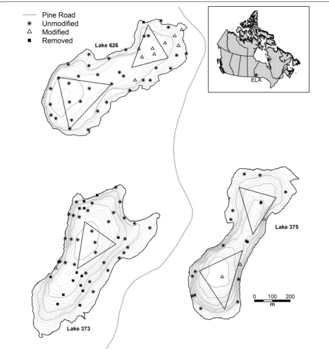
potential buoy drift, and GPS coordinates were checked regularly throughout the open water season. The triads were linked to an onshore computer via radio link, which allowed for real-time monitoring of acoustic tag signals. A more complete description of the RAPT systems is provided by Blanchfield et al. [7, 13]. In Lake 375, two separate RAPT systems were in operation, one each in the north and south basins (Fig. 1). A single RAPT system was in operation in Lake 373, positioned over the deepest part of the lake to maximize the number of detections of tagged, cold-water-adapted lake trout (Fig. 1). Two RAPT systems were in operation in Lake 626, one in the west basin and the other in the east basin (Fig. 1). Individual RAPT buoys were re-positioned in the same location as the previous year during each open water period to maintain consistency.
Stationary tag trials
Stationary tag trials were performed to test the accu-racy and precision of the RAPT systems (Fig. 1). Each stationary location consisted of an anchor, a line to the surface, and a float. For deployment, a tag was placed in a plastic bottle with holes in it to allow water to flow through, and the bottle was attached to the anchor line at a known depth. Tags were deployed at each location for ~24–72 h except for rare circumstances where tags were left at stations for more than 1 week. The location of each stationary tag trial was recorded using a hand-held GPS unit (GPSMap76 or GPSMap60CSX; measurement error reported by the GPS units for all locations was 2–4 m). Beginning in the fall of 2005, stationary trials were con-ducted in Lake 375. Three tags were used at 19 stations around the lake, most of which fell outside the RAPT triads. Only one stationary trial was deployed within the north triad in Lake 375, and this tag was placed near an experimental aquaculture cage. Unfortunately, during the early stages of this experiment the focus was to (1) deter-mine whether the RAPT system could detect tags near the shoreline and (2) identify sources of error outside the triads with less attention paid to the error structure within the triad so we have limited information about the error structure within the triads on Lake 375. The spatial trials were improved upon for Lakes 373 and 626 by expanding the number of stations and placing more emphasis within the triads, but nearshore areas were still considered important. The stationary tag trials carried out in Lake 373 (summer 2009 and fall 2013), employed 12 tags and 46 stations. Some stations in Lake 373 were sampled at multiple depths to test whether depth affected positioning. The stationary tag trials performed in Lake 626 in 2010 and 2013 used 15 tags in 45 locations. We retested three locations in the spring of 2015 in Lake 373 to examine potential temporal changes in data quality.
Assumptions
We used the following assumptions for hydro-acoustic systems:
(1) There is no inter-tag variation in detection quality (2) Depth does not affect telemetry positioning
(3) Water temperature (seasonal effect) or thermocline does not affect acoustic signals travelling through the water
(4) The errors will display temporal consistency, and thus, a single stationary tag trial is sufficient for cor-recting multiple years of data
(5) The error structure of the detections follows a bivar-iate Gaussian distribution
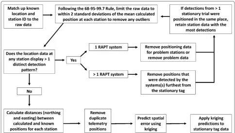
Correcting the data
easting and northing Euclidean distances in relation to the actual position of the stationary tag. To quantify the spa-tial error of the RAPT systems, ordinary kriging (simply termed kriging hereafter) was employed through the use of the R statistical package geoR [14].
Validation of the kriging method
We used a fivefold cross-validation to test the predict-ability of the kriging method. In fivefold cross-validation, the data set gets partitioned randomly into five equally sized subdata sets, and one subsample is taken as the testing set and the remaining subsamples are used as the model training set. The training set is used as input into the kriging method, and the testing set is used to test the predictability of the model. The process is repeated five times to independently use each subsample as the test-ing set. Further validation was performed in Lake 373 by a “leave-one-out” procedure “Appendix”). This procedure involved sequentially removing one station from the data set, performing the kriging method, and calculating the spatial error on the raw and corrected data.
Depth comparison
During the course of the stationary tag trials, efforts were made to test whether tag depth affected the positioning ability of the RAPT systems. Depth tests were conducted in both Lake 373 and Lake 375, but no thermocline was
present in Lake 375 during the test. We felt it was most important to present results with tags set above and below a thermocline to show whether changes in water density has an effect on signal propagation, and thus, we have only included depth test results from Lake 373. To measure spatial overlap between tags set at different depths, we calculated the 95 % kernel home range for each depth and measured home range overlap using the volume of intersection statistic (VI). The VI was intro-duced by Seidel [15] and compares the utilization distri-bution (UD) overlap between two animals (from Fieberg and Kochanny [16]):
The VI ranges from zero (for 2 home ranges with no over-lap) to 1 (for 2 home ranges with overlapping uniform UDs). The VI has been suggested as a preferred method of assessing UD overlap based on theoretical grounds as well as from a simulation performed by Fieberg and Kochanny [16].
State‑space models
State-space models are used to estimate the state of unob-served processes from observations while accounting for measurement errors and stochasticity in the process [17].
VI =
∞∞
−∞−∞
minUD1
x,y,UD2
x,ydxdy
In the present case of this study, the true location is the unobserved process. As is common with many remote sensing methods for geolocation data, there are latitudinal and longitudinal variances (measurement errors) asso-ciated with the observed location. We can use a SSM to account for the variances of the observed locations while simultaneously using maximum likelihood to estimate an animal’s true position. In the context of this study, we have assumed that the measurement errors follow a bivariate normal distribution around the mean spatial coordinates from each stationary tag trial. To model telemetry posi-tions in continuous time, we followed methods described by Johnson et al. [18] to put a continuous-time correlated random walk model into a SSM framework. The telem-etry data collected for this study differ from Argos data in that the quality class for each detection is not recorded, and thus, we assume measurement errors display a Gauss-ian structure for all detections within the SSM frame-work where the mean and standard deviation are fixed. Although we understand that telemetry systems can be subject to dilution of precision, in the context of our study we decided to treat all detections with equal weight since only the highest quality data were retained during pro-cessing. In order to estimate the SSM parameters, we used the crawl package [12].
Performance of correction techniques
To assess the quality of data, we spatially quantified sys-tematic errors using kriging and used the SSM to correct measurement errors. We tested the performance of each method independently and simultaneously and quanti-fied the improvements. Using observed telemetry data from a tagged lake trout in each of the three study lakes, we present four scenarios: (1) raw data, (2) data corrected for measurement error (only SSM), (3) data corrected for systematic error (only kriging), and (4) data corrected for both measurement and systematic errors. In order to compare the performance of each scenario, we used three indicators to measure activity and space use: total dis-tance travelled, 100 % home range size calculated using the minimum convex polygon (MCP) [19], and 50 % ker-nel density estimator (KDE) [20]. We used the adehabi-tatHR library [21] to calculate the MCP and KDE using the R statistical language. We chose to use the MCP method to describe the absolute home range and a KDE for detecting biologically important areas [22]. Total dis-tance travelled was used to show how biases in the telem-etry data can influence calculations in animal behaviour and bioenergetics. For the purpose of this study, we have assumed that there is no spatial variation in detection quality among stationary tag locations. Thus, we model bias as varying in space and treat measurement error as equal among all locations.
Results
Stationary tag trials
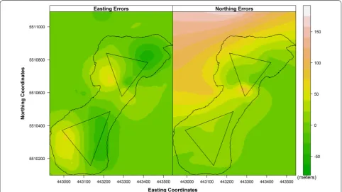
Stationary tag trials were used to assess spatial error of RAPT systems, and a spherical covariance model was used to describe the easting errors and northing errors in the study lakes (Fig. 3). Table 1 summarizes data from the stationary tag trials in all three test lakes. Of 24 338 detections in Lake 375, a total of 12 995 positions were removed from the analysis. Although this is a large num-ber of detections, closer inspection reveals that a sin-gle station in Lake 375 was removed from analysis with a total of 11 616 detections (47.7 % of total detections). In this case, three tags were simultaneously deployed at the same station in an area between two RAPT systems and left for 29 days, but the RAPT systems were not able to consistently position the tags during this trial; thus, the accumulated data were omitted. It is expected that these tags were in a “shadow zone” where the tag could be detected, but the receivers were not able to cleanly pick up the signal, and the distribution of detections resembled a long-axis along the fetch of Lake 375. Of the remaining positions in Lake 375, a total of 10 960 (96.6 %) detections were spatial duplicates. In Lakes 373 and 626, the percent of spatially duplicate detections were 94.6 and 97.7 %, respectively. This high proportion of duplica-tion indicates that the RAPT systems are able to posiduplica-tion tags with a high degree of precision.
In Lake 375, the mean northing error was 33.35 m and the mean easting error was 32.93 m from the true tag locations. Overall, the mean systematic error (Euclidean distance) in Lake 375 was 50.15 m. The RAPT positions of stationary tags display a high degree of precision (the data points are clustered), but there was considerable systematic error (the clusters of points do not match the known tag locations) (Fig. 3a). Closer inspection of three stations within Lake 375 (Fig. 3b–d) illustrates the spa-tial distribution of the positioning errors. In each case, the RAPT systems show low accuracy but good preci-sion. Similar results were obtained in Lakes 373 and 626 in relation to the precision of the systems, but the sys-tematic errors were much different. Of the three lakes studied, the system on Lake 373 produced the most sys-tematic bias, which was most likely due to a combination of bathymetry and distance of stationary tags from the centre of the triad.
Correcting spatial error
When we applied the northing and easting corrections generated by the kriging technique to the raw data pro-duced by the RAPT systems, the accuracy of the spatial positions improved considerably (Table 2, kriged posi-tions). The corrected data in Lake 375 had a mean north-ing error of 0.28 m and a mean eastnorth-ing error of 0.35 m.
(kriged; an improvement of 97 %). During the initial analysis of Lake 626, we found that the performance of the RAPT systems was superior to that of the other two lakes with a mean systematic error of 12.2 m. The kriging technique was able to position stationary transmitters to 0.79 m away from their known location, for an improve-ment of 94 %. Although the percent improveimprove-ment on Lake 626 was the smallest of the three study lakes, the initial performance was very high compared to the other lakes.
Depth comparison
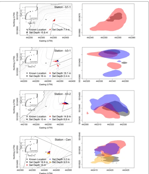
System performance was affected by the depth of tag placement (Tables 3, 4). Accuracy of the system was affected less than precision, as tags set at different depths still displayed VI index values ≫0 in most cases. The only location where tags displayed a relatively low overlap val-ues is where the tag was set at 3.2 m at centre buoy in
Lake 373 (“Cen” station). For all other depths and loca-tions around Lake 373, the VI values ranged from 0.26 to 0.32. Although these values are much lower than a com-plete overlap as indicated by a value of 1, the size of the 95 % UD used to calculate the VI index varied greatly (Table 3). Since the UD can be thought of a three-dimen-sional representation describing where an animal can be found at any point in time, centres of high use receive added weight during comparisons. We can see from Fig. 5 that a tag does behave slightly differently at vari-ous depths. Interestingly, for the depth comparisons con-ducted on Lake 373 the tags set at the deepest depth all exhibited the smallest home range (Table 4). It is possible that signals emitted from tags located near the surface are exposed to a certain degree a backscatter, resulting in higher degree of inaccuracy. Our depth trials were con-ducted over multiple years in Lake 373 as well as above and below a thermocline (Fig. 5). The results from our
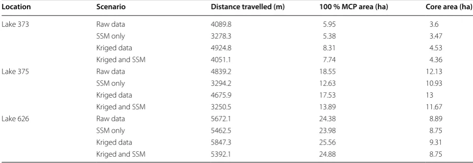
Table 1 Summary of stationary tag trial data for RAPT systems in Lakes 373, 375, and 626 at the Experimental Lakes Area
Lake Maximum
depth (m) Area (ha) # tags # stations # stations used in kriging # detections # detections removed # duplicate detections
373 21 27.3 14 47 33 39,708 15,826 22,583
375 26 23 3 19 18 24,338 12,995 10,960
626 12 26.2 15 45 44 97,963 45,065 51,671
depth trials indicate that depth does have an effect on the RAPT systems, but this effect is not significant enough to suggest that either assumption 2 or assumption 3 was violated. The performance of the system from year
to year is consistent, and therefore, we also assume that assumption 4 is valid.
Comparing correction techniques
We used tracking data from a tagged lake trout in each of the three study lakes to demonstrate how different scenarios for error correction can influence data col-lected irregularly through time (Table 5). Using the raw data reported by the RAPT system in Lake 375, the total
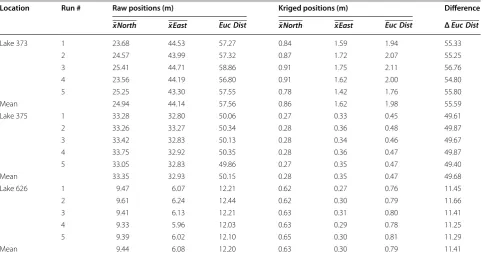
Table 2 Summary of fivefold cross-validation of the kriging model
Mean northings (x North) and eastings (¯ x East) are distances of detections from known tag locations. The Euclidean distance (Euc Dist) is distance between locations ¯ calculated by the RAPT system and the actual tag location. The change in Euclidean distance (ΔEuc Dist) is the difference between the raw and kriged tag positions
Location Run # Raw positions (m) Kriged positions (m) Difference
¯
xNorth xEast¯ Euc Dist xNorth¯ xEast¯ Euc Dist Δ Euc Dist
Lake 373 1 23.68 44.53 57.27 0.84 1.59 1.94 55.33
2 24.57 43.99 57.32 0.87 1.72 2.07 55.25
3 25.41 44.71 58.86 0.91 1.75 2.11 56.76
4 23.56 44.19 56.80 0.91 1.62 2.00 54.80
5 25.25 43.30 57.55 0.78 1.42 1.76 55.80
Mean 24.94 44.14 57.56 0.86 1.62 1.98 55.59
Lake 375 1 33.28 32.80 50.06 0.27 0.33 0.45 49.61
2 33.26 33.27 50.34 0.28 0.36 0.48 49.87
3 33.42 32.83 50.13 0.28 0.34 0.46 49.67
4 33.75 32.92 50.35 0.28 0.36 0.47 49.87
5 33.05 32.83 49.86 0.27 0.35 0.47 49.40
Mean 33.35 32.93 50.15 0.28 0.35 0.47 49.68
Lake 626 1 9.47 6.07 12.21 0.62 0.27 0.76 11.45
2 9.61 6.24 12.44 0.62 0.30 0.79 11.66
3 9.41 6.13 12.21 0.63 0.31 0.80 11.41
4 9.33 5.96 12.03 0.63 0.29 0.78 11.25
5 9.39 6.02 12.10 0.65 0.30 0.81 11.29
Mean 9.44 6.08 12.20 0.63 0.30 0.79 11.41
Table 3 Comparison of 95 % kernel home range overlap for tags set at different depths using the volume of inter-section statistic (VI) for four stations in Lake 373
Tags were set at identical spatial locations, but depth of the tag in the water column was different for each trial. Depths 1 and 2 represent the comparison used to attain each VI value (0 = no overlap, 1 = for 2 home ranges with overlapping uniform UDs)
Station Depth 1 (m) Depth 2 (m) VI
b1-1 7.4 15.8 0.26
b3-1 2.4 16 0.30
2.4 15 0.35
15 16 0.12
b3-2 8.8 15 0.28
8.8 14.8 0.08
14.8 15 0.15
Cen 3.2 9.5 0.06
3.2 15 0.71
3.2 16.9 0.003
9.5 15 0.05
9.5 16.9 0.31
15 16.9 0.006
Table 4 95 % kernel home range for each depth trial at each station in Lake 373
Station Tag depth (m) Area (m2)
b1-1 7.4 104
15.8 18
b3-1 2.4 670
15 424
16 140
b3-2 8.8 278
14.8 169
15 154
Cen 3.2 51
9.5 40
15 69
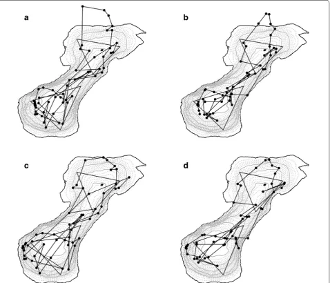
distance travelled by a lake trout was 4839 m, the ker-nel home range size was 12.13 ha, and the MCP home range size was 18.55 ha (Fig. 6a, Table 5). Where we used a SSM to correct the measurement errors (scenario 2), the total distance travelled was 3294 m, the kernel home range size was 10.93 ha, and the MCP home range was 12.63 ha (Fig. 6b). In the third scenario, where the raw data were corrected by kriging, we observed a total dis-tance travelled of 4676 m, a kernel home range of 13 ha, and a MCP home range of 17.53 ha (Fig. 6c). When we applied a SSM to the kriged data, (scenario 4), total dis-tance travelled by the lake trout was 3251 m, the kernel home range was 11.67 ha, and the MCP home range was 13.89 ha (Fig. 6d). Depending on the error correc-tion scenario applied, estimates of distance travelled by lake trout ranged from 32 % lower to 20 % greater than calculated from raw data. Similarly, MCP of lake trout ranged from 32 % smaller to 40 % larger than that calcu-lated from raw data, and core-use areas were up to 10 % smaller and 26 % larger than estimates from raw telem-etry data. Results from each lake suggest that only apply-ing a SSM to raw data results in a contraction in all three of our performance indicators. The application of kriging (scenario 3) and the combination of kriging and a SSM (scenario 4) produced more complex results. In Lake 373, the MCP and kernel density area increased in scenar-ios 3 and 4, but the total distance increased in scenario 3 and decreased in scenario 4. In Lake 375, all three of our performance indicators decreased with the applica-tion of correcapplica-tion techniques. In Lake 626, the lake where the systems produced the highest quality results from the raw data, the correction techniques produced similar
results to the raw data. Scenario 3 showed increased val-ues for all three performance indicators, while scenario 4 had decreased distance travelled and core area use, but greater MCP area (Table 5).
Discussion
Acoustic telemetry is a widely used method of gathering spatial distribution data for organisms in aquatic envi-ronments. It is generally accepted that RAPT systems have a certain amount of intrinsic error associated with them likely resulting from deployment in complex acous-tic environments. When assessing important ecological questions like an animal’s home range, it is important to use accurate spatial positioning information. As such, we have identified a need to quantify and correct systematic biases produced by acoustic telemetry systems. Through the use of stationary tag trials and kriging, we have suc-cessfully modelled errors inherent in acoustic telemetry methods using systems from three lakes in the Canadian boreal shield, removing systematic biases and improving the accuracy of the spatial data. We chose kriging because it is well documented in the literature, straightforward to use, and worked well for our purpose. Other spatial inter-polation methods such as a general additive model [23] could be explored by other researchers depending on their data structure and experimental design. Further-more, we have shown that kriging can be combined with SSMs to correct measurement errors as well. The general conclusion of this study is that the systematic errors pro-duced by the RAPT systems have a greater effect on the quality of the data compared to the measurement errors and so we believe that more effort should be applied to
Table 5 Performance of error correction techniques applied to raw RAPT data of an acoustically tagged lake trout ( Salve-linus namaycush) in three different lakes at the Experimental Lakes Area
Each of the four scenarios is quantified by the total distance travelled by a fish, the 100 % minimum convex polygon (MCP) to indicate total space use, and the kernel density core area use (50 %) to quantify areas of high importance
Location Scenario Distance travelled (m) 100 % MCP area (ha) Core area (ha)
Lake 373 Raw data 4089.8 5.95 3.6
SSM only 3278.3 5.38 3.47
Kriged data 4924.8 8.31 4.53
Kriged and SSM 4051.1 7.74 4.36
Lake 375 Raw data 4839.2 18.55 12.13
SSM only 3294.2 12.63 10.93
Kriged data 4675.9 17.53 13
Kriged and SSM 3250.5 13.89 11.67
Lake 626 Raw data 5672.1 24.38 8.89
SSM only 5462.5 23.98 8.75
Kriged data 5847.3 25.56 9.31
performing stationary tag trials to identify problem areas in study systems. We feel that the measurement error dis-played by the RAPT systems in our study lakes is of lesser concern and that the quality of the data is most affected by systematic biases.
The depth of a stationary tag clearly affected the detec-tion quality during the tag trials, but this effect had greater implications for precision than accuracy. The low degree of overlap calculated by the VI should not be a cause for concern because the VI uses three-dimensional space use in its calculation. Even at centre buoy where the shallow tag did not have high overlap with the deeper tags, the absolute difference between the mean software-derived locations for each depth was within ~5 m of each other. On an ecosystem level, an error of 5 m would not have a dramatic impact on space use and home range size. Signals that are transmitted from tags near the surface are likely subject to reflections from the surface waters. Signals in an aquatic environment are analogous to signals travelling down a canyon, where the canyon walls can reflect signals, but in the case of a freshwater or marine system one of the “walls” (the surface of the water) is a dynamic interface affected by wind and other environmental factors [24]. Similar results were obtained by Baktoft et al. [25], where the authors tested an acous-tic telemetry system on two lakes. The depth trials sug-gest that space use of tagged animals that inhabit the upper water column may be considerably overestimated compared to those living deeper in the water column. Furthermore, detections from the depth trials (Fig. 5, Table 4) show that the presence of a thermocline did not have a negative effect on the acoustic signal; therefore, we did not violate assumptions 2 or 3. In our case, the acous-tic signals were unaffected by a thermal barrier, but per-haps the signals may be more sensitive in systems with a chemical barrier or other physical barrier; if so, a sepa-rate stationary tag trial may need to be conducted above and below the disturbance to determine whether separate corrections would be required.
For our purposes, we have defined our errors using an absolute measure of error in metres in two dimensions (northing and easting). An additional way to report errors currently in use by VPS is termed horizontal positioning error (HPE). In the framework of HPE, the arrival time of a signal from a transmitter to two receivers defines a branch of a hyperbola; this branch is commonly termed a hyperbolic line of position (LOP). A transmitter can be located along any point of this LOP with the actual mitter location unknown. In order to calculate a trans-mitter location, a second hyperbola is calculated from a third receiver. The intersection point of these two LOPs is the location of the transmitter. See Smith [2] for fur-ther details about the hyperbolic positioning sensitivity,
especially Figs. 4, 5 and 6. One of the main drawbacks of using HPE is that it should only be interpreted as a unit-less estimate of error sensitivity while HPEm (measured horizontal position error estimate in metres) should only be used for informal purposes [2]. The performance of the VPS system was tested in marine, estuary, and river-ine environments with median HPEm of 3.3 m and less although system performance was not tested outside of the arrays [26]. In the context of our study, we were able to specifically quantify the positioning error in two dimensions, which allowed us to use the kriging method to create the error maps in Fig. 4. We did not, however, have access to estimates for error sensitivity for our analysis. Although HPE cannot be used for error correc-tion purposes, it does provide researchers informacorrec-tion regarding the quality of the detections and can be used to identify areas where more receivers could be placed. Many aquatic species use nearshore areas for breeding and foraging. These areas often have important biological implications, but depending on receiver or RAPT buoy placement, these areas may receive relatively poor cov-erage, and thus, the error sensitivity (HPE) may be high. The kriging method returns much more informative error information than HPEm because although HPEm returns information relative to the accuracy of a detec-tion it does not provide anything about the direcdetec-tionality of the error. The kriging method can quantify the preci-sion error in two dimenpreci-sions, which in turn can be used to identify complex habitat or problem areas.
In multi-species systems, researchers may want to monitor more than one species at a time using acoustic telemetry. Different species may have different physi-ological constraints, and in turn they may need to inhabit different niches within the water column. The depth tri-als we performed showed that tags detected closer to the surface were subject to “backscattering” issues, which caused higher detection variation. Consider a hypotheti-cal system that contains two distinct species where one is a warm-water-adapted species (species A) and a sec-ond cold-water-adapted fish (species B). During periods of stratification when species B is driven deeper into the lake due to metabolic requirements and species A is unaffected, based on our results, data quality from spe-cies A would be considerably less, with respect to trans-mitter precision, than that of species B, and it is likely that energetic estimates would also be overestimated for species A. This type of scenario deserves some considera-tion when designing a study monitoring species with dif-ferent habitat and metabolic requirements.
results suggest that home ranges can also be underesti-mated. In our study, the RAPT systems did not have a consistent bias throughout the lake. RAPT systems either incorrectly positioned tags closer to or further from the centre of the triad, but not in a consistent fashion. In addition, RAPT systems are used in both freshwater [8] and marine systems [27, 28], but it is presently unknown whether RAPT systems deployed in marine systems pro-duce the same patterns of bias that are present in fresh-water systems. The method we developed in this paper aims to reduce the effects associated with telemetry errors by increasing the accuracy of the estimated posi-tions and to simultaneously quantify and correct any
biases produced by the system. In small lakes like the ones commonly present in the boreal and arctic regions, this underestimation could have a large impact on the ratio of surface area to core space use.
The utilization of a SSM is meant to account for the measurement errors of the detections. In some cases, it became apparent that the measurement errors became more variable along one axis, and in these cases the northing errors were different from the easting errors (e.g. Fig. 3b vs. c). This phenomenon was shown by Espi-noza et al. [1] regarding tag placement inside and outside an array. The pattern detected by their VPS system is very similar to patterns detected by the RAPT systems in our Fig. 6 A comparison of raw data three corrections applied to acoustic positioning telemetry data of a free-ranging lake trout (Salvelinus namaycush) in Lake 375 at the Experimental Lakes Area, monitored by two RAPT systems (see Fig. 1) over a period of approximately 24 h. The panels show: a
study when transmitters were located far from the cen-tre of the triads. In our study, a normal distribution was used to describe the error structure of the detections in the SSM, but [25] used a hidden Markov model (HMM) and a t-distribution to model measurement errors (the authors refer to them as observation errors). Although this technique did not address any systematic biases that may have been present, this approach did improve the data (with some residual scattering around the true positions). Perhaps in the future a combination of krig-ing to address the systematic bias and a t-distribution in a SSM to address the measurement errors may further improve telemetry data by accounting for spatial differ-ences in measurement errors. Although we feel the need to account for measurement errors in RAPT data is rela-tively low due to the high precision as seen in the station-ary tag trials, the fact that this type of data is collected irregularly through time presents yet another statistical challenge for analysis.
The principle of RAPT systems relies on arrival times of acoustic signals from tags to hydrophones. In our sys-tem in order for a tag to be positioned, the signal from a tag is detected by three omnidirectional hydrophones, and the arrival times of the acoustic signals are processed and run through “signal-arrival-time” difference equa-tions, which are used to calculate the tag position [28, 29]. Some of the factors that must be taken into consid-eration in the origin of measurement errors are the speed of sound through water and arrival-time differences [30]. Environmental variables may also contribute to meas-urement errors. Wind action causes waves, which can distort sound signals and cause anchored buoys to shift from their recorded. In our study, any unrecorded small-scale movement of the hydrophones could potentially add more noise during the signal arrival time, but the method by which the buoys were anchored limited their movement. All telemetry systems are subject to these disturbances; we controlled these variables as much as possible by mooring the buoys solidly. Receiver locations should be chosen to maximize lake coverage while mini-mizing potential interactions of acoustic signals (e.g. cliffs or large boulders) while continuing to maximize detec-tion probability of the study species.
Recommendations
The kriging methodology proposed in this paper is a simple, yet powerful way to correct systematic errors in acoustic telemetry systems. Though some time and effort must be expended to perform a stationary tag trial in an experimental system, in our opinion the benefits out-weigh the costs in order to achieve the most accurate telemetry data for aquatic species that are otherwise diffi-cult to study on a continuous timescale. The results from
the kriging analyses are likely to be robust and could be used to correct systematic errors over multiple years. The application of this method affects research areas such as bioenergetics, habitat utilization, and resource use. The ability and flexibility of this method to be used in lakes with one or more RAPT systems should allow other researchers to reduce the influence of problem telem-etry data and thus increase the accuracy of inferred fish positions and movement. Regarding our three scenarios of spatial correction, we found that the kriging method had the best performance with regard to spatial correc-tion. On its own, the SSM was not able to identify or compensate for the bias present in our study systems. At this point, it is unknown whether there is any advantage to combining the kriging and SSM solely on the reality that detection quality was not returned with the sys-tem presented in this paper. Temporal stability should be further tested by leaving tags at stationary locations for longer periods of time, possibly for the length of the study or just a single year. This would allow researchers to adjust for seasonal effects that were not apparent dur-ing the deployment of our tags. Alternately, researchers could conduct multiple short-term trials throughout the year (e.g. 1 week per month); this would yield stationary tag data that are temporally spaced, but would reduce the load on the telemetry system and the effort required on the part of the researcher to process the data.
In closing, we found that the systematic errors were more likely to influence the recorded position of the sta-tionary tags rather than measurement errors. Although SSMs can be used to correct measurement errors, in the context of our study the SSM on its own was not able to compensate for biases introduced by the interaction between the physical environment and the telemetry sys-tem. Therefore, we recommend that any future telemetry studies should perform at least a rudimentary stationary tag trial in order to assess the performance of their sys-tem. Any such trials should attempt to cover as much of the study area as possible, with multiple stations located within each triad of receivers and many nearshore loca-tions. It is especially important to conduct trials near areas of expected biological importance in order to draw accurate biological conclusions.
Authors’ contributions
CC was involved in data collection, statistical analysis, interpretation of data, and drafting the manuscript. DMG was involved in the conception of the methods developed in this manuscript, revising the manuscript, and inter-pretation of data. LEH contributed to the design of the experiment, revising the manuscript, and acquisition of data. PJB was involved in study design, conception of the methods, acquisition of data, and revising the manuscript. All authors read and approved the final manuscript.
Author details
Acknowledgements
We appreciate the field support of L. Tate, L. Cruz-Font, F. Bjornson, J. Cederwall, A. Chapelsky, D. Callaghan, M. Guzzo as well as other ELA staff and students. Funding for this study was provided by Fisheries and Oceans Canada, the Experimental Lakes Graduate Fellowship, and IISD Experimental Lakes Area, Inc.
Competing interests
The authors declare that they have no competing interests.
Appendix
“Leave‑one‑out” kriging performance test
In order to validate the kriging method further, we also tested it using a “leave-one-out” quality control. This method involves sequentially removing one station from the data set, running the kriging process with the remain-ing stations, and applyremain-ing the resultremain-ing correction map to the data from the removed station. This was performed on all stations within the lake. This allowed us to test the krig-ing method on data from “unknown” data points, while still having access to the known transmitter location, thus allowing us to quantify the accuracy of the kriging process.
The “leave-one-out” method showed bias improve-ment at all but 5 stations on Lake 373. Further, at 3 of these 5 stations tags were displaced less than 4 m; the maximum value for stations where the kriging method did not improve the raw data was 19.6 m (Fig. 7). The kriging method was able to improve the data quality for the remaining 28 stations (85 % of all stations). Mean improvement was 50.8 m (median of 50.83 m), while the mean error at stations where the kriging method did not improve the data quality was 8.4 m (median of 3.8 m).
Figure 8 illustrates the results of the leave-one-out proce-dure for each station on Lake 373.
Although the performance was not improved at all stations, the benefits of applying the kriging procedure outweigh the costs. Stations within the triad were not improved by the kriging process, but these stations gen-erally provided the most reliable positioning data. This suggests that correction by kriging is less important for positions detected within the buoy triad. The “leave-one-out” method clearly showed that stations near the perime-ter of the lake were more likely to be influenced positively by the kriging method where there is strong evidence for over- or under-correction. These results show that kriging produces much more reliable data outside of the triad (vs. raw data); the “kriged” positions are much closer to the actual tag position than the “raw” data. This method of quality control reinforces that stations must be tested out-side of the triads, especially near shore where biologically important habitats may be located in order to properly address and assess telemetry errors. The leave-one-out procedure showed that kriging is essential to yield accu-rate data outside the triad and that kriging has minimal effects on high-quality data within the triads.
Effect of grid size and detection filtering
During the development of our correction technique, we identified two crucial factors, which directly affect Fig. 7 This figure shows the results of the “leave-one-out” method.
The black line shows the 1:1 ratio for the original error and the kriged error. All points which lie to the right of the 1:1 line show an improve-ment in Euclidean distance from the actual tag position compared to the raw data (blue points), while points to the left of the line were made worse by kriging (red points)
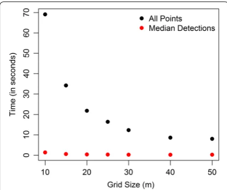
processing time: (1) number of detections and (2) grid size. The kriging method required creating a spatial grid over the study area in order to assign error estimates to each grid. This grid was used for linear interpolation of spatial bias from the RAPT system. The choice of grid size and the number of accumulated points at each sta-tion affected the processing time. Improvements in technology, including battery life, receiver memory stor-age, and tag ping intervals of <30 s, have increased the potential for long-term remote telemetry studies to yield massive data sets. Even in this study where the tags emit-ted signals every 120–300 s and detections were filtered to only include data within 2 standard deviation of the mean at each station (~95 % of the data), each station still produced a high number of detections (up to 2000 detections at a single station). Using these detections, the limiting factor was selecting grid size for interpolation (Fig. 9). Processing times ranged from ~10 s per station using a 50-m grid to 70 s per station using a 10-m grid. Increasing the grid size led to an exponential decline in processing time, and these limitations were readily evi-dent when using the “leave-one-out” method. In Lake 373 where we used 33 stations, the total processing time could take longer than 40 min.
In future large-scale studies that involve stationary tag trials, processing time will become the limiting fac-tor. One way to improve processing time would be to use the median detection location for each stationary tag rather than the entire cloud of detection points when producing the kriging map. The median detection loca-tion represents the central tendency of the data, and it is
less sensitive to outliers and could be used to represent all detections at that stationary location. In our study, the use of the median location for each station in the krig-ing technique yielded processkrig-ing times of only a few sec-onds per station for all grid sizes and produces a 51-fold improvement in processing time using a grid size of 10 m.
Received: 19 September 2015 Accepted: 20 January 2016
References
1. Espinoza M, Farrugia TJ, Webber DM, Smith F, Lowe CG. Testing a new acoustic telemetry technique to quantify long-term, fine-scale move-ments of aquatic animals. Fish Res. 2011;108:364–71.
2. Smith F. Understanding HPE in the VEMCO positioning system (VPS) V1.0, September 27, 2013. http://vemco.com/wp-content/uploads/2013/09/ understanding-hpe-vps.pdf. Document #: DOC-005457-01. Retrieved 15 Jan 2015.
3. Begout Anras ML, Cooley PM, Bodaly RA, Anras L, Fudge RJP. Movement and habitat use by lake whitefish during spawning in a boreal lake: inte-grating acoustic telemetry and geographic information systems. Trans Am Fish Soc. 1999;128:939–52.
4. Zamora L, Moreno-Amich R. Quantifying the activity and movement of perch in a temperate lake by integrating acoustic telemetry and a geographic information system. Hydrobiologia. 2002;483:209–18. 5. Espeland SH, Gundersen AF, Olsen EM, Knutsen H, Gjøsæter J, Stenseth
NC. Home range and elevated egg densities within an inshore spawning ground of coastal cod. ICES J Mar Sci. 2007;64:920–8.
6. Andrews KS, Tolimieri N, Williams GD, Samhouri JF, Harvey CJ, Levin PS. Comparison of fine-scale acoustic monitoring systems using home range size of a demersal fish. Mar Biol. 2011;158:2377–87.
7. Blanchfield PJ, Flavelle LS, Hodge TF, Orihel DM. The response of lake trout to manual tracking. Trans Am Fish Soc. 2005;134:346–55.
8. Blanchfield P, Tate L, Podemski C. Survival and behaviour of rainbow trout (Oncorhynchus mykiss) released from an experimental aquaculture opera-tion. Can J Fish Aquat Sci. 2009;66:1976–88.
9. Journel AG, Huijbregts CJ. Mining Geostatistics. New York: Academic Press; 1978.
10. Jonsen I, Flemming J, Myers R. Robust state-space modeling of animal movement data. Ecology. 2005;86(11):2874–80.
11. R Core Team. R: a language and environment for statistical computing. R Foundation for Statistical Computing, Vienna, Austria; 2014. http:// www.R-project.org/.
12. Johnson DS. crawl: Fit continuous-time correlated random walk models to animal movement data. R package version 1.4-1.2013. http://CRAN.R-project.org/package=crawl.
13. Blanchfield PJ, Tate LS, Plumb JM, Acolas M-LA, Beaty KG. Seasonal habitat selection by lake trout (Salvelinus namaycush) in a Canadian shield lake: constraints imposed by winter conditions. Aquat Ecol. 2009;43:777–87. 14. Ribeiro PJ Jr, Diggle PJ. geoR: a package for geostatistical analysis.
R-NEWS. 2001;1(2):15–8.
15. Seidel KS. Statistical properties and applications of a new measure of joint space use for wildlife. Thesis, University of Washington, Seattle, USA. 1992. 16. Fieberg J, Kochanny CO. Quantifying home-range overlap: the
impor-tance of the utilization distribution. J Wildl Manage. 2005;69(4):1346–59. 17. Jonsen I, Myers R, Flemming J. Meta-analysis of animal movement using
state-space models. Ecology. 2003;84:3055–63.
18. Johnson DS, London JM, Lea MA, Durban JW. Continuous-time correlated random walk model for animal telemetry data. Ecology. 2008;89:1208–15. 19. Mohr CO. Table of equivalent populations of North American small
mam-mals. Am Mid. Nat. 1947;37:223–49.
20. Worton BJ. Kernel methods for estimating the utilization distribution in home-range studies. Ecology. 1989;70:164–8.
21. Calenge C. The package adehabitat for the R software: a tool for the analysis of space and habitat use by animals. Ecol Model. 2006;197:516–9. Fig. 9 Processing time for a single station using a range of grid
• We accept pre-submission inquiries
• Our selector tool helps you to find the most relevant journal • We provide round the clock customer support
• Convenient online submission • Thorough peer review
• Inclusion in PubMed and all major indexing services • Maximum visibility for your research
Submit your manuscript at www.biomedcentral.com/submit
Submit your next manuscript to BioMed Central
and we will help you at every step:
22. Nilsen EB, Perdersen S, Linnell JDC. Can minimum convex polygon home ranges be used to draw biologically meaningful conclusions? Ecol Res. 2008;23:635–9.
23. Wood SN. Generalized additive models: an introduction with R. London: Chapman and Hall/CRC; 2006.
24. Caley M, Duncan A. Conceptual development of a dynamic underwater acoustic channel simulator. Paper number 134. Proceedings of ACOUS-TICS 2011. 2011.
25. Baktoft H, Zajicek P, Klefoth T, Svendsen JC, Jacobsen L, Pedersen MW, Morla DM, Skov C, Nakayama S, Arlinghaus A. Performance assessment of two whole-lake acoustic positional telemetry systems—Is reality min-ing of free-range aquatic animals technologically possible? PLoS One. 2015;10(5):20.
26. Steel AE, Hearn AR, Klimley AP. Performance of an ultrasonic telemetry positioning system under varied environmental conditions. Anim Bio-telem. 2014;2(15):1–17.
27. Rigby PR, Andrade Y, O’Dor RK. Interpreting behavioural data from radio–acoustic positioning telemetry (RAPT) systems. Afr J Mar Sci. 2005;27(2):395–9.
28. Voegeli FA, Smale MJ, Webber DM, Andrade Y, O’Dor RK. Ultrasonic telem-etry, tracking and automated monitoring technology for sharks. Environ Biol Fish. 2001;60:267–81.
29. O’Dor RK, Andrade Y, Webber DM, Sauer WHH, Roberts MJ, Smale MJ, Voegeli FM. Applications and performance of radio–acoustic positioning and telemetry (RAPT) systems. Hydrobiologia. 1998;371(372):1–8. 30. Ehrenberg JE, Steig TW. Improved techniques for studying the