Shape Properties of Irregular Surface Data
Maria Hussain
Department of Mathematics
Lahore College for Women for University, Lahore, Pakistan [email protected]
Malik Zawwar Hussain
Department of Mathematics
University of the Punjab, Lahore, Pakistan [email protected]
Iram Butt
Department of Mathematics
University of the Punjab, Lahore, Pakistan
Abstract
The presented work of this paper addresses the two shape properties, positivity and monotonicity of irregular surface data. The data is initially triangulated and a side-vertex scheme is adopted to interpolate the data over each triangle. Each boundary and radial curve is a rational function with three parameters facilitating 18 parameters in each triangular patch. The presence of these parameters leads to an automotive scheme for shape preservation and shape control. The data dependent constraints are derived on 6 of these parameters for preservation of positive and monotone properties of data, while, remaining 12 are free for shape modification. This scheme is local, does not constrain step length and derivatives, equally applicable to both data and data with derivatives.
Keywords: Rational cubic function, Triangular patch, Shape parameters, Positivity, Monotonicity.
AMS Subject Classification 2000:68U05, 65D05, 65D07, 65D18.
1. Introduction
The development of interpolation and approximation techniques which address the problem of shape preservation and control is one of the sought areas of Computer Graphics. The properties of data, whether gathered experimental or physical, can be categorized as positive, monotone and convex. Ordinary interpolation techniques guarantee smoothness but do not concentrate whether the shape properties of data are also inherited by developed curves and surfaces.
couples in statistics, empirical option pricing model in finance and approximation of potential functions in physical and chemical systems (Beliakov, 2005).
The limitation of ordinary interpolation techniques leads to the problem of shape preserving interpolation discussed by a number of authors. Chan and Ong (Chan and Ong, 2001) involved the cubic Bézier triangular interpolant for range restricted interpolation of irregular surface data. The derived sufficient conditions imposed restrictions on Bézier ordinates to give non-negative cubic Bézier triangular patch. The interpolating surface is a convex combination of these patches. If the Bézier ordinates did not satisfy the imposed restriction then it was remedied by scaling of first order partial derivatives at vertices. Piah, Goodman and Unsworth (Piah et al., 2005) also used cubic Bézier triangular interpolant to preserve the shape of irregular surface data. The derivatives at data sites were computed to be consistent with these conditions. Piah et al., (2006) addressed the problem of range restricted interpolation using quartic Bézier triangular interpolant which was an extension of (Piah et al., 2005). Each triangular patch was the convex combination of three quartic Bézier triangular patches. Again the positivity was ensured by a set of restriction on Bézier ordinates. Hussain and Hussain (2010, 2011) used rational function with parameters to preserve the positive and monotone shape of irregular surface data. Hussain and Hussain (2010, 2011) developed data dependent constraints on these parameters to preserve the positive and monotone shape of data and no parameter were free for shape refinement. Mulansky and Schmidt (1994) used quadratic spline on a Powell-Sabin refinement of triangulation to generate a constrained interpolant. Utreras (1985) defined a method that how positivity can be treated as a constraint, providing a global optimization at each step of iteration, but its computational cost was high.
Beliakov (2005) introduced a method for monotone interpolation and smoothing of irregular surface data. Monotonicity constraints were applied on noisy data to make it smooth and change it into a quadratic programming problem. This method was only useful to preserve the shape of monotone Lipschitz continuous function. Han and Schumaker (1997) scheme addressed the monotonicity of irregular surface data. The given irregular surface data was arranged over rectangular grids. The demerit of this method was that a system of N -irregular surface data points reduced to N2- rectangles.
Moreover, a few of these were very small in one or both directions. Goodman et al., (1995) proposed derivative estimation scheme for scattered data.
The piecewise rational cubic function (Sarfraz, et al., 1997) having three shape parameters generates the radial and boundary curves of each triangular patch. Each triangular patch has six shape preserving parameters and twelve free parameters for shape refinement. The subject of the paper is to develop local positive and monotone irregular surface data interpolation schemes which do not constrain step length and derivatives.
a rational function with parameters is developed for irregular surface data interpolation. The problems of positive and monotone data interpolation are discussed in Section 3.2 and 3.3 respectively. Section 4 demonstrates the results developed in the previous sections. Section 5 concludes the paper.
2. Cubic Hermite Interpolation of Irregular Surface Data
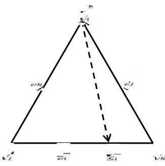
Fig. 1.Location of the vertices and edges of the triangle VV Vi j k.
This section provides a review of irregular surface data interpolation scheme proposed by Nielson (1979). The primary requirement was to arrange the data over the triangular grid such that each data point was the vertex of some triangle. The partial derivatives at the vertices of triangle were computed. The data at the three boundaries of a triangle were interpolated by cubic Hermite spline. The rational interpolant of each triangle was a convex combination of radial curves, the curves joining the vertex to the opposite edge of the triangle. The radial curves were also obtained by cubic Hermite interpolation. For any triangleVV Vi j k, with barycentric coordinates u, v andw, any point V
x y, on thetriangle can be expressed as:
i j k
V uV vV wV , u v w 1 and u v w, , 0 (1)
The Nielson side-vertex interpolant, interpolating the irregular data arranged over a triangular patch was expressed by the following convex combination:
2 2 2 2 2 2
2 2 2 2 2 2
( , , ) v w RC u w RC u v RCi j k P u v w
v w u w u v
. (2)
i
RC , RCj and RCk were the radial curves connecting the vertices Vi, Vj and Vk to the
opposite edges ei, ej andek. The order of continuity achieved by Nielson scheme was 1
At the vertices of the triangle VV Vi j k where two of the barycentric coordinates are
simultaneously zero, the P u v w
, ,
is defined as
,0,0
1P u Z , P
0, ,0v
Z2, P
0,0,w
Z3,where Zi, i1,2,3 are the ordinate values at the vertices Vi, Vj and Vk respectively.
3. Shape Properties of Irregular Surface Data
In this section, shape preserving interpolation schemes are developed to interpolate the positive and monotone irregular surface data. The data is triangulated by Delaunay triangulation method (Fang and Piegl, 1992). The Nielson side-vertex interpolation scheme by Nielson (1979) is used to interpolate the data over the each triangle with the modification that each boundary curve and each radial curve is the rational cubic function (Sarfraz et al., 1997). Both positivity and monotonicity preserving schemes have developed constraints on parameters to preserve the shape of data.
3.1 Rational interpolant for irregular surface data
Let {( , , ),x y Z ii i i 1,2,3,..., }n be the given set of irregular data arranged over the triangulated grid. Without the loss of generality we shall consider an arbitrary triangle
i j k VV V
, and will construct the rational interpolant overVV Vi j k. The edges of VV Vi j k
opposite to the vertices Vi, Vj, Vk are ei, ej and ek respectively. Arbitrary points of the
edges ei, ej and ek are denoted by Si, Sj and Sk. Let RCi, RCj and RCk be the radial
curves joining the vertices Vi, Vj, Vk to the edgesei, ej and ek respectively. Zi,
1,2,3
i are the ordinate values at vertices Vi, Vj, Vk respectively. The radial curve RCi
connecting the vertex Vi to the point Si on the opposite boundary edge ei is defined as in
i
id RC RC
RC
, (3)
3 2
3
2
2 21 1 2 3 4
(1 ) 1 1
in i i i i i
RC u u u A Z u u uA BC S u v D u w D
1 2
(1 ) i (1 ) i
u u v D u u w D
,
1 ( i i)
A , A2 ( i i),
22 1 1
id i i i
RC u u u u ,
1 j i BC i j i BC i
D x x S y y S
x y
,
2 k i BC i k i BC i
D x x S y y S
x y
,
3 j i F i j i F i
D x x V y y V
x y
,
4 k i F i k i F i
D x x V y y V
x y
13 1 2 12
1 1
2 1 3
1 2
1 1
3 1 4
3 1 32 2
1 1 1 1
i
s Z s s Z d s s Z d s Z
BC S
s s s s
, (4)
3 k j F j k j F j
d x x V y y V
x y
,
4 k j F k k j F k
d x x V y y V
x y , 1 v s v w , w s v w .
Similarly, the radial curves connecting the vertices Vj and Vk to the edges ej and ekare
defined as jn j jd RC RC RC
, (5)
3 2
3
2
2 21 2 2 7 8
1 1 1
jn j j j j j
RC v v v B Z v v vB BC S v u D v w D
1
j 5
1
j 6v v u D v v w D
,
22 2 1 1
jd j j j
RC v v v v ,
1 ( j j)
B , B2 (j j),
5 i j BC j i j BC j
D x x S y y S
x y
,
6 ( k j) BC j k j BC j
D x x S y y S
x y
,
7 i j F j i j F j
D x x V y y V
x y
,
8 ( k j) F j k j F j
D x x V y y V
x y
,
13 1 3 12
2 2
3 2 5
1 2
2 2
1 2 6
3 2 12 2
2 1 1 1
j
r Z r r Z d rr Z d r Z
BC S
r rr r
, (6)
5 i k F k i k F k
d x x V y y V
x y
,
6 i k F i i k F i
d x x V y y V
x y , 1 w r u w , u r u w . kn k kd RC RC RC
, (7)
3 2
3
2
2 21 3 2 11 12
1 1 1
kn k k k k k
RC w w w C Z w w wC BS S w u D w v D
1
k 9
1
k 10w w u D w w v D
22 1 1
kd k k k
RC w w w w ,
1 ( k k)
C , C2 (k k),
9 i k BC k i k BC k
D x x S y y S
x y
,
10 j k BC k j k BC k
D x x S y y S
x y
,
11 i k F k i k F k
D x x V y y V
x y
,
12 j k F k j k F k
D x x V y y V
x y
,
13 3 1 12
3 3
1 3 1
1 2
3 3
2 3 2
3 3 22 2
3 1 1 3
k
t Z t t Z d t t Z d t Z
BC S
t t t t
, (8)
1 j i F i j i F i
d x x V y y V
x y
,
2 j i F j j i F j
d x x V y y V
x y
,
1 u
t
u v
,
v t
u v
.
The parameters i, j, k, 1, 2, 3, i, j, k, 1, 2, 3, i, j, k, 1, 2 and
3
are parameters known as shape design parameters used to modify the shape of surface as required. The rational interpolant over each triangular patch is constructed by substituting the values RCi, RCj and RCk from (3), (5) and (7) in (2).
3.2 Positivity preserving interpolation of irregular surface data
Let {( , , ),x y Z ii i i 1,2,3,..., }n be the given irregular data, positive over the whole domain (Zi 0,i1, 2,3,...,n).
The rational interpolant (2) will be positive if each of the boundary curve defined in (3), (5) and (7) are positive. The radial curvesRCi, RCj and RCk can be rearranged as:
in i
id RC RC
RC
,
where
3 2
2 2 32 1 1 2 3 4 5 6
1 1
in i i i
RC u u u A BC S Z vG wG v G vwG w G v G
2 7
v wG 2 3
8 9
vw G w G
, (9)
22 1 1
id i i i
RC u u u u , (10)
1 3 i 1 1 1 i 3
G Z A Z D ,
2 3 i 1 1 1 i 4
G Z A Z D ,
3 i 1 2 1 1 i 1 2 i 3
4 6 i 1 4 1 1 i 1 i 2 2 i 3 2 i 4
G Z A Z D D D D ,
5 3 i 1 2 1 1 i 2 2 i 4
G Z A Z D D ,
6 i 1 1 1 i 1 i 3
G Z A Z D D ,
7 3 i 1 3 1 1 2 i 1 i 2 2 i 3 i 4
G Z A Z D D D D ,
8 3 i 1 3 1 1 2 i 2 i 1 2 i 4 i 3
G Z A Z D D D D ,
9 i 1 1 1 i 2 i 4
G Z A Z D D ,
jn j
jd
RC RC
RC
,
3 2
2 2 32 2 1 2 3 4 5 6
1 1
jn j j j
RC v v vB BC S Z uL wL u L uwL w L u L
2 7
u wL 2 3
8 9
uw L w L
, (11)
22 1 1
jd j j j
RC v v v v , (12)
1 3 j 2 1 2 j 7 L Z B Z D ,
2 3 j 2 1 2 j 8 L Z B Z D ,
3 3 j 2 2 1 2 j 5 2 j 7 L Z B Z D D ,
4 6 j 2 4 1 2 j 5 j 6 2 j 7 2 j 8 L Z B Z D D D D ,
5 3 j 2 2 1 2 j 6 2 j 8 L Z B Z D D ,
6 j 2 1 2 j 5 j 7
L Z B Z D D ,
7 3 j 2 3 1 2 2 j 5 j 6 2 j 7 j 8 L Z B Z D D D D ,
8 3 j 2 3 1 2 2 j 6 j 5 2 j 8 j 7 L Z B Z D D D D ,
9 j 2 1 2 j 6 j 8
L Z B Z D D ,
kn k
kd RC RC
RC
,
3 2
2 22 3 1 2 3 4 5
1 1
kn k k k
RC w w wC BC S Z uM vM u M uvM v M
3 6
u M 3 9
8 2 7
2vM uv M v M
u , (13)
22 1 1
kd k k k
RC w w w w , (14)
1 3 k 3 1 3 k 11
M Z C Z D ,
2 3 k 3 1 3 k 12
M Z C Z D ,
3 3 k 3 2 1 3 k 9 2 k 11
M Z C Z D D ,
4 6 k 3 4 1 3 k 9 k 10 2 k 11 2 k 12
M Z C Z D D D D ,
5 3 k 3 2 1 3 k 10 2 k 12
M Z C Z D D ,
6 k 3 1 3 k 9 k 11
M Z C Z D D ,
7 3 k 3 3 1 3 2 k 9 k 10 2 k 11 k 12
M Z C Z D D D D ,
8 3 k 3 3 1 3 2 k 10 k 9 2 k 12 k 11
M Z C Z D D D D ,
9 k 3 1 3 k 10 k 12
0
i
RC if RCin 0 and RCid 0.
From (9), RCin 0 if i 0, i 0, BC S( ) 0i and Gi 0, i1, 2,3,...,9.
From (10), RCid 0 if i 0, i 0 and i 0.
Using Theorem developed in (Sarfraz, Al-Mulhem and Ashraf, 1997), BC S( ) 0i if
3 4 1
2 3
0, d d,
Max Z Z , 0 i
G , i1, 2,3,...,9 if
1 3 1 4 1 3
1 1 1
2 2
0, i i , i i , i i ,
i Max ZZ D ZZ D DZ D
2 4 1 ,
iD iD Z
1 2 3 4 2 1 4 3
1 1
(2 ) (2 ), (2 ) (2 )
3 3
i D D i D D i D D i D D
Z Z
and
1 3 1 2 4 1 1 2 3 4 1
1 1 1
2 2 ( ) 2 ( ) 2
0, , ,
2 2 4
i i i i i i i i i
i Min D ZD Z D ZD Z D D ZD D Z
.
Similarly, RCj 0if 5 6
2
3 1
0, d d,
Max Z Z , 0 i
L , i1, 2,3,...,9 if
2 7 2 8 5 7 6 8
2 2 2 2
2 2
0, j j , j j , j j , j j ,
j
Z D Z D D D D D
Max
Z Z Z Z
5 6 7 8 6 5 8 7
2 2
(2 ) (2 ) (2 ) (2 )
,
3 3
j D D j D D j D D j D D
Z Z
and
5 7 2 6 8 2 5 6 7 8 2
2 2 2
2 2 ( ) 2 ( ) 2
0, , ,
2 2 4
j j j j j j j j j
j
D D Z D D Z D D D D Z
Min
Z Z Z
Similarly, RCk 0, if 1 2
3
1 2
0, d d,
Max Z Z , 0 i
M , i1, 2,3,...,9 if
3 11 3 12 9 11 10 12
3 3 3 3
2 2
0, k k , k k , k k , k k ,
k Max ZZ D Z Z D DZ D DZ D
9 10 11 12 10 9 12 11
3 3
(2 ) (2 ), (2 ) (2 )
3 3
k D D k D D k D D k D D
Z Z
and
9 11 3 10 12 3 9 10 11 12 3
3 3 3
2 2 ( ) 2 ( ) 2
0, , ,
2 2 4
k k k k k k k k k
k Min D ZD Z D ZD Z D D ZD D Z
The above discussion is summarized as:
Theorem 1. The C1 triangular patch, defined over the triangular domain in (2), is
positive if the following sufficient conditions are satisfied:
1 i 2
1 3 1 4 1 3 1
1 1 1
2 2
0, iZ iD , iZ iD , iD iD ,
Q Max
Z Z Z
2 4 1 ,
iD iD Z
1 2 3 4 2 1 4 3
1 1
(2 ) (2 ), (2 ) (2 )
3 3
i D D i D D i D D i D D
Z Z
,
1 3 1 2 4 1 1 2 3 4 1
2
1 1 1
2 2 ( ) 2 ( ) 2
0, , ,
2 2 4
iD iD iZ iD iD iZ i D D i D D iZ
Q Min
Z Z Z
,
2 7 2 8 5 7 6 8
3
2 2 2 2
2 2
0, jZ jD , jZ jD , jD jD , jD jD ,
Q Max
Z Z Z Z
5 6 7 8 6 5 8 7
2 2
(2 ) (2 ) (2 ) (2 )
,
3 3
j D D j D D j D D j D D
Z Z
,
5 7 2 6 8 2 5 6 7 8 2
4
2 2 2
2 2 ( ) 2 ( ) 2
0, , ,
2 2 4
jD jD jZ jD jD jZ j D D j D D jZ
Q Min
Z Z Z
,
3 11 3 12 9 11 10 12
5
3 3 3 3
2 2
0, kZ kD , kZ kD , kD kD , kD kD ,
Q Max
Z Z Z Z
9 10 11 12 10 9 12 11
3 3
(2 ) (2 ), (2 ) (2 )
3 3
k D D k D D k D D k D D
Z Z
,
9 11 3 10 12 3 9 10 11 12 3
6
3 3 3
2 2 ( ) 2 ( ) 2
0, , ,
2 2 4
kD kD kZ kD kD kZ k D D k D D kZ
Q Min
Z Z Z
.
3.3 Monotonicity preserving interpolation of irregular surface data
In this section, we shall establish the sufficient conditions for the monotonicity of rational interpolant (2) in an arbitrary direction d 1 1V 2 2V 3 3V , 1 2 3 0.
(Floater and Peña, 2000) stated:
Definition 1. A function f x y
, is said to be strictly monotone in any direction d if
, 0d
D f x y ,
where Dd denotes the directional derivative along the directiond.
Let
x y Z ii, ,i i
, 1,2,3
be the monotone irregular surface data defined over thetriangle VV Vi j k obeying the restrictions that if x xi j andyi yj then Zi Zj and
0
x l
Z and y 0
l
Z , l i j k , , .
The directional derivative of (2) along the direction d 1 1V 2 2V 3 3V , with 1
2 3 0
is
1 2 3 d N
d
d
D P
P P P
D P
u v w D P
2 4 2 4 2 2 4 4 4 4 2 4 2 2 4 4 21 2 3 4 5 6 7
d N
D P u v w E u v w E u v E v w E uv w E u v w E uv w E
4 4 8
u w E 2 4 2 4 4 2 4 2
9 10 11 12
u vw E u v wE u vw E u v wE
, (16)
2 2 2 2 2 2
2 d DD P u v v w w u (17)
i
E , i1,2,3,...,12can be obtained by simple computation involved in (15). Using the Definition (1), the rational interpolant (2) is monotone if D Pd 0.
D Pd
D 0is positive always, whereas,
D Pd
N 0 if Ei 0, i1,2,3,...,12.0
i
E , i1,2,3,...,12 if 0
id
RC , with i1, 2, 3, i 0, i 0, i 0; i1,2,3,...17.
1 RCj RCi 0
, 1
RC RCk i
0, 2
RCkRCj
0, 3
RC RCi k
0,
2 RCk RCj 0
, 3
RCj RCk
0,i 0, i 0, i 0 ; i1,2,3,...17.
0, 1, 8
1 Max Coni i
, 2 Max
0,Coni,9i16
,
0, ,17 24
3 Max Coni i
, 4 Max
0,Coni,25i30
,
0, ,31 36
5 Max Coni i
, 6 Max
0,Coni,37i42
,where
2 1 3 2 1 1
1
1 1 2 3 3 4
( ) 2 ( ( ))
2 ( ( )) ( )
i i i
i
D D Z BC S
Con
Z BC S D D
,
1 1 2 3 3 4
2
1 1
4 ( ( )) ( )
( ( ))
i i i
i
Z BC S D D
Con
Z BC S
,
2 1 3 2 1 1
3
1 1
( ) ( ( ))
( i ( ))i i i
D D Z BC S
Con
Z BC S
,
2 1 3 2 1 1
4
1 1
( ) 2 ( ( ))
2 ( ( ))
i i i
i
D D Z BC S
Con
Z BC S
, 1 5 3 iD Con D , 2 6 4 , iD Con D 1 3 7 3
( 2 )
i D D Con D , 2 4 8 4
( 2 )
i D D Con
D
,
1 5 3 6 2 2
9
2 2 1 7 3 8
( ) 2 ( ( ))
2 ( ( )) ( )
j j j
j
D D Z BC S
Con
Z BC S D D
,
2 2 1 7 3 8
10
2 2
4 ( ( )) ( )
( ( ))
j j j
j
Z BC S D D
Con
Z BC S
1 5 3 6 2 2 11
2 2
( ) ( ( ))
( ( ))
j j j
j
D D Z BC S
Con
Z BC S
,
1 5 3 6 2 2
12
2 2
( ) 2 ( ( ))
2 ( ( ))
j j j
j
D D Z BC S
Con
Z BC S
, 5 13 7 jD Con D , 6 14 8 jD Con D , 5 7 15 7
( 2 )
j D D
Con D , 6 8 16 8
( 2 )
j D D
Con
D
,
1 9 2 10 3 3
17
3 3 1 11 2 12
( ) 2 ( ( ))
2 ( ( )) ( )
k k k
k
D D Z BC S
Con
Z BC S D D
,
3 3 1 11 2 12
18
3 3
4 ( ( )) ( )
( ( ))
k k k
k
Z BC S D D
Con
Z BC S
,
1 9 2 10 3 3
19
3 3
( ) ( ( ))
( k ( ))k k k
D D Z BC S
Con
Z BC S
,
1 9 2 10 3 3
20
3 3
( ) 2 ( ( ))
2 ( ( ))
k k k
k
D D Z BC S
Con
Z BC S
, 9 21 11 , kD Con D 10 22 12 kD Con D , 9 11 23 11
( 2 )
k D D Con D , 10 12 24 12
( 2 )
k D D Con
D
,
2 1 3 3 1 3 2 3 1 4 25
3 3 2
2 ( ) 2
2 ( )
d Z Z d
Con Z Z ,
3 1 3 2 3 1 3 2
26
3 3 2
2 ( )
( )
d Z Z
Con Z Z ,
3 1 4 3 1 3 2 2 1 4 27
3 4
3 ( ) 2
d Z Z d
Con d ,
2 1 4 1 3 2 3 2 1 2 3
28
2 2 3
2 ( ) ( )
( )
d Z Z Z Z
3 1 3 2 1 3 2 1 2 3 29
2 3
2 d d 3 (Z Z )
Con d ,
2 1 3 3 1 4 2 1 3 2 30
2 2 3
2 2 ( )
2 ( )
d d Z Z
Con Z Z ,
3 2 5 1 2 1 3 1 2 6 31
1 1 3
2 ( ) 2
2 ( )
d Z Z d
Con Z Z ,
1 2 5 3 1 2 1 3
32
1 1 3
2 ( )
( )
d Z Z
Con Z Z ,
1 2 6 1 2 1 3 3 2 6 33
1 6
3 ( ) 2
d Z Z d
Con d ,
3 2 6 2 1 3 1 3 2 3 1
34
3 3 1
2 ( ) ( )
( )
d Z Z Z Z
Con Z Z ,
1 2 5 3 2 5 3 2 3 1 35
3 5
2 d d 3 (Z Z )
Con d ,
3 2 5 1 2 6 3 2 1 3 36
3 3 1
2 2 ( )
2 ( )
d d Z Z
Con Z Z ,
1 3 1 2 3 2 1 2 3 2
37
2 2 1
2 ( ) 2
2 ( )
d Z Z d
Con Z Z ,
2 3 1 1 2 3 1 2
38
2 2 1
2 ( )
( )
d Z Z
Con Z Z ,
2 3 2 2 3 2 1 1 3 2
39
2 2
3 ( ) 2
d Z Z d
Con d ,
1 3 2 3 2 1 2 1 3 1 2
40
1 1 2
2 ( ) ( )
( )
d Z Z Z Z
Con Z Z ,
2 3 1 1 3 1 1 3 1 2 41
1 1
2 d d 3 (Z Z )
Con d ,
1 3 1 2 3 2 1 3 2 1 42
1 1 2
2 2 ( )
2 ( )
d d Z Z
Con Z Z .
The above discussion is summarized as:
Theorem 2. The triangular patch P, defined over the triangular domain, in (2), is monotone in the direction d 1 1V 2 2V 3 3V , with 1 2 3 0 if the following conditions are satisfied
1 p Max1 0,Coni,1 i 8
, 2 p Max2
0,Coni,9 i 16
,
3 p Max3 0,Coni,11 i 24
, 4 p Max4
0,Coni,25 i 30
,
5 p Max5 0,Coni,31 i 36
, 6 p Max6
0,Coni,37 i 42
,4. Numerical Examples
In this section, the shape preserving interpolating scheme developed in Section 3 is implemented on some functions.
Example 1. The positive irregular surface data is generated from the following positive function
, 1
2 0.21 x y xy
F ,
and the domain is restricted to
4,4
4,4
. Figs. 2 and 3 show the Delaunay triangulation of the domain and linear interpolation of the positive irregular surface data generated from the functionF x y1
,
. Fig.4 is generated from the interpolating scheme,discussed in Section 3 for the value of shape parameters 1 2 3 1 2 3 i
1
j k i j k
and i j k 1 2 3 2 which reduces the
given interpolant to the cubic Hermite triangular interpolant. Fig. 5 is another view of Fig.4. Figs. 4 and 5 show that some part of the surface lie below the plane Z 0, it means that it only interpolates the data but does not preserve the shape of the positive irregular surface data. Fig.6. is generated from Theorem 1 with free parameters
3 . 1
3 2 1 3 2
1 i j k i j k
. In Fig.6, it is to be
noted that the shape of the positive irregular surface data is preserved. Fig.7 provides another view of Fig.6.
Example 2. The next example is also for the positive irregular surface data generated from the following function
2 , 2 xy
F x y x y+e sin(y),
and domain is restricted to
0,3 0,3 . Figs. 8 and 9 represent the Delaunay triangulation and linear interpolation of the irregular surface data generated from the function F x y2
,
.Fig.10 is the cubic Hermite triangular surface of the given function and we observed that cubic Hermite did not preserve the shape of positive data. Fig.11 is another view of Fig.10. Fig.12 is generated from the Theorem 1 for the free parameters are
1 2 3 1 2 3 i j k i
j k 1.22 and the surface generated from this scheme is positive. Fig.13 is another view of Fig.12.
Example 3. The monotone irregular surface data are generated from the following function
3 , 2 2
F x y x+ln x + y -1.5,
and domain is restricted to
1, 10 1, 10
. Figs. 14 and 15 are the Delaunay triangulation and linear interpolation of the monotone irregular surface data. Fig.16. is the cubic Hermite triangular surface and by using the Hermite interpolant, the surface deviates from its monotone behaviour. Figs. 17 and 18 are the xz-view and yz-view of the Fig.16. Fig.19. is generated from Theorem 2 for the values of free parameters1 2 3 1 2 3 i j k i j k
Example 4.The fourth example is also for the monotone irregular surface data generated from the following function
4 ,
F x y = ln 2x+ y+1 .
The domain is restricted to
0, 5 0, 5 . Fig. 22 and 23 are the Delaunay triangulation of the domain and linear interpolation of the irregular data generated from the function
4 ,
F x y . Fig.24. is the cubic Hermite triangular surface and it does not preserve the shape of monotone data. Figs 25 and 26 are the xz-view and yz-view of the Fig.24. Fig.27 is generated from Theorem 2 and values of shape parameters are
1 2 3 1 2 3 i j k i j k 0.05
. Monotone shape of the data has been preserved in Fig.27. Figs. 28 and 29 are the xz-view and yz-view of Fig.27.
Fig.2.Triangulation of the domainF x y1
,
. Fig.3.Linear interpolation of F x y1
,
.Fig.6.Positive side-vertex interpolantofF x y1
,
. Fig.7.Another view of Fig.6.Fig.8.Triangulation of the domainF x y2
,
. Fig.9.Linear interpolation ofF x y2
,
.Fig.12.Positive side-vertex interpolantof F x y2
,
. Fig.13.Another view of Fig.12.Fig.14.Triangulation of the domain F x y3
,
. Fig.15.Linear interpolation ofF x y3
,
.Fig.18.yz-view of Fig.16. Fig.19.Monotone side-vertex interpolantof F x y3
,
.Fig.20.xz-view of Fig.19. Fig.21.yz-view of Fig.19.
Fig.24.Hermite triangular surface of F x y4
,
Fig.25.xz-view of Fig.24.Fig.26.yz-view of Fig.24. Fig.27.Monotone side-vertex interpolantof F x y4
,
.5. Conclusion
In (Beatson and Ziegler, 1985, Chan and Ong, 2001, Piah, Goodman and Unsworth, 2005, Piah, Saaban and Majid, 2006), constraints are derived on derivatives. When derivatives are given with data then these schemes are not helpful. But in this paper, the scheme is acceptable to both data with and without derivatives. In (Hussain, et al, 2009), a piecewise rational cubic function with one free parameter is used. This scheme does not give the freedom to the user to modify the shape of the data. In this paper, 12 shape parameters in each triangular patch are free for user choice to modify the shape of the data.
The monotonicity preserving scheme presented in (Beliakov, 2005) is only applicable to Lipschitz continuous functions. In (Han and Schumaker, 1997) the given irregular data is arranged to rectangular grid but the schemes of this paper are acceptable to both rectangular and triangular grid.
References
1. Beatson, R.K. and Ziegler, Z. (1985). Monotonicity preserving surface interpolation,SIAM Journal on Numerical Analysis,22(2), 401-411.
2. Beliakov, G. (2005). Monotonicity preserving approximation of multivariate scattered data,BIT,45, 653-677.
3. Chan, E.S. and Ong, B.H. (2001). Range restricted scattered data interpolation using convex combination of cubic Bézier triangles, Journal of Computational
and Applied Mathematics, 136, 135-147.
4. Fang, T.P. and Piegl, L.A. (1992). Algorithms for Delaunay triangulation and convex-hull computation using a sparse matrix, Computer Aided Design, 24, 425- 436.
5. Floater, M.S. and Peña, J.M. (2000). Monotonicity preservation on triangles,
Mathematics of Computation,69 (232), 1505-1519.
6. Goodman, T.N.T., Said, H.B. and Chang, L.H.T. (1995). Local derivative estimation for scattered data interpolation, Applied Mathematics and
Computation,68, 41- 50.
7. Han, L. and Schumaker, L.L. (1997). Fitting monotone surfaces to scattered data using piecewise cubic,SIAM Journal of Numerical Analysis, 23(2), 569-585. 8. Hussain, M.Z., Sarfraz, M. and Butt, S. (1997). Non-negative rational spline
interpolation, Proceedings of First International Conference on Information Visualization (IV’97), August 27-29, 1997, London, UK, 200-204.
9. Hussain, M.Z. and Hussain, M. (2009). Shape preserving scattered data interpolation,European Journal of Scientific Research,25(1), 151-164.
10. Hussain, M.Z. and Hussain, M. (2010). C1 positive scattered data interpolation,
Computers and Mathematics with Applications, 59, 457-467.
11. Hussain, M.Z. and Hussain, M. (2010). C1 monotone scattered data interpolation,
Transactions on Computational ScienceVIII,LNCS6260, 156-166.
13. Nielson, G. (1979). The side-vertex method for interpolation in triangles, Journal
of Approximation Theory, 25, 318-336.
14. Piah, A.R.M., Goodman, T.N.T. and Unsworth, K. (2005). Positivity-preserving scattered data interpolation,Lecture Notes in Computer Science,3604, 336- 349. 15. Piah, A.R.M., Saaban, A. and Majid, A.A. (2006). Positivity preserving scattered
data interpolation,Lecture Notes in Computer Science,3604,63-75.
16. Sarfraz, M., Al-Mulhem, M. and Ashraf. F. (1997). Preserving monotonic shape of the data using piecewise rational cubic functions, Computers & Graphics, 21(1), 5-14.
17. Utreras, F.I. (1985). Positive thin plate splines,Journal of Approximation Theory