M E T H O D O L O G Y
Open Access
GAMETES: a fast, direct algorithm for
generating pure, strict, epistatic models with
random architectures
Ryan J Urbanowicz, Jeff Kiralis, Nicholas A Sinnott-Armstrong, Tamra Heberling, Jonathan M Fisher
and Jason H Moore
**Correspondence:
[email protected] Department of Genetics, Institute for Quantitative Biomedical Sciences, Dartmouth Medical School, Lebanon, NH, USA
Abstract
Background: Geneticists who look beyond single locus disease associations require additional strategies for the detection of complex multi-locus effects. Epistasis, a multi-locus masking effect, presents a particular challenge, and has been the target of bioinformatic development. Thorough evaluation of new algorithms calls for
simulation studies in which known disease models are sought. To date, the best methods for generating simulated multi-locus epistatic models rely on genetic algorithms. However, such methods are computationally expensive, difficult to adapt to multiple objectives, and unlikely to yield models with a precise form of epistasis which we refer to as pure and strict. Purely and strictly epistatic models constitute the worst-case in terms of detecting disease associations, since such associations may only be observed if alln-loci are included in the disease model. This makes them an
attractive gold standard for simulation studies considering complex multi-locus effects. Results: We introduce GAMETES, a user-friendly software package and algorithm which generates complex biallelic single nucleotide polymorphism (SNP) disease models for simulation studies. GAMETES rapidly and precisely generates random, pure, strictn-locus models with specified genetic constraints. These constraints include heritability, minor allele frequencies of the SNPs, and population prevalence. GAMETES also includes a simple dataset simulation strategy which may be utilized to rapidly generate an archive of simulated datasets for given genetic models. We highlight the utility and limitations of GAMETES with an example simulation study using MDR, an algorithm designed to detect epistasis.
Conclusions: GAMETES is a fast, flexible, and precise tool for generating complex
n-locus models with random architectures. While GAMETES has a limited ability to generate models with higher heritabilities, it is proficient at generating the lower heritability models typically used in simulation studies evaluating new algorithms. In addition, the GAMETES modeling strategy may be flexibly combined with any dataset simulation strategy. Beyond dataset simulation, GAMETES could be employed to pursue theoretical characterization of genetic models and epistasis.
Keywords: GAMETES, SNP, Epistasis, Simulation, Model, Genetics
Background
Despite the rising quality and abundance of genetic data, epidemiologists continue to struggle to explain the known heritability of these complex phenotypes with existing
genetic factors. While strategies seeking single locus associations (i.e. main effects) are often sufficient to address diseases which follow Mendelian patterns of inheritance, their application to diseases characterized as complex has yielded limited success in the pur-suit of explaining heritability [1,2]. Epistasis is one of several phenomena reviewed by [3] believed to hinder the reliable identification of predictive genetic markers in association studies. The termepistasiswas coined to describe a genetic “masking” effect viewed as a multi-locus extension of the dominance phenomenon, where a variant at one locus pre-vents the variant at another locus from manifesting its effect [4]. In the present study we consider statistical epistasis, which is the phenomenon as it would be observed in asso-ciation studies. Statistical epistasis is traditionally defined as a deviation from additivity in a mathematical model summarizing the relationship between multi-locus genotypes and phenotypic variation in a population [5]. Specifically, we focus on statistical epistasis that is bothstrictandpure. Ann-locus model is purely and strictly epistatic if allnloci, but no fewer, are predictive of disease status. The loci in these models could be viewed as “fully masked” in that no predictive information is gained until allnloci are considered in concert.
Computational geneticists are putting significant effort into developing algorithms for the detection of complex disease associations within clinical data [6-9]. While real biological datasets serve as the gold standard for validating new techniques, the development and systematic evaluation of computational strategies calls for simulated data.
Previous genetic data simulation efforts have introduced strategies for generating dif-ferent data types including: quantitative trait loci mapping [10], pedigree association [11-15], and case/control-based association [16-23]. The simulation of datasets typically involves two stages: model generation, and sample generation. While most of the strate-gies cited above focus on the latter stage, the generation of realistic complex disease models constitutes a key challenge.
Moore, et. al [18] noted that simple, biallelic, 1-locus or purely epistatic 2-locus models of disease can be assembled with relative ease via trial and error. [24] char-acterized all fully penetrant two-locus models, where genotype disease probabilities were restricted to zero and one [25], later expanded upon this to include models with continuous penetrance values [26], generated purely epistatic models using the double description method [27] (for 2-locus models) and a non-linear maximization strategy (for 3 and 4-locus models) [17] and [18], recruited an evolutionary algorithm (EA) to evolve 2 to 5-locus epistatic models encoded as binary chromosomes. Over succes-sive generations, models evolved towards a state of pure epistasis. Most recently, [23] circumvented the typical first stage of data simulation (i.e. model generation), directly evolving the genotypes and affection status of samples in a dataset. Evolving datasets with 3 to 5 SNPs at a time, this EA strategy evolved 3 to 5-locus epistatic inter-actions while attempting to avoid main effects and any intermediate nested 2-locus interactions.
the EA fitness landscape becomes multi-objective, introducing further challenges and limitations to the evolutionary process.
In this study we introduce a Genetic Architecture Model Emulator for Testing and Evaluating Software (GAMETES). This algorithm provides a direct approach for the sim-ulation of biallelicn-locus epistatic models which may be used in conjunction with any sample generation strategy. Specifically, GAMETES generates a precise class of epistatic models that are both pure and strict. Eachn-locus model is generated deterministically, based on a set of random parameters, a randomly selected direction, and specified values of heritability, minor allele frequencies, and (optionally) population disease prevalence. For valid combinations of these model constraints, GAMETES attempts to generate a population of model architectures. We use the termarchitectureto reference the unique composition of a model (i.e. the penetrance values and arrangement of those values across genotypes). We demonstrate that GAMETES is a fast, reliable, and flexible method for generating complex genetic models of random architecture. We evaluate GAMETES over an example simulation study using MDR [28], an exhaustive combinatorial search algorithm designed to detect epistasis.
Methods
In this section, we describe (1) relevant background in genetics and modeling, (2) the specific steps for generatingn-locus epistatic models that are both strict and pure and (3) an example simulation study using GAMETES.
Genetics and modeling
Single nucleotide polymorphisms (SNPs) are single loci in the DNA sequence where alter-nate nucleotides (i.e. alleles) are observed between members of a species or between paired chromosomes in an individual. Most characterized SNPs are biallelic, meaning that only two alleles (Aora) are observed in a population. The genotype of a SNP in a diploid organism is determined by alleles found on each chromosome of the homologous pair. A biallelic SNP can have one of three genotypes:AA,Aa, oraa. The termgenotype
has been used to refer both to the allele states of a single SNP, as well as the combined allele states of multiple SNPs. To avoid confusion, we refer to the latter as a multi-locus genotype (MLG) whenever necessary.
SNPs not under selective pressure within a population typically exhibit genotype fre-quencies that are predicted by the Hardy-Weinberg Law [29]. Like most data simulation strategies, GAMETES adopts the assumption of Hardy-Weinberg Equilibrium (HWE) such that the allele frequencies of a SNP may be used to calculate it’s genotype frequencies as follows: freq(AA)=p2, freq(Aa)=2pq, and freq(aa)=q2, wherepis the frequency of the major (more common) allele ‘A’,qis the minor allele frequency (MAF) of the minor allele ‘a’, andp+q=1. GAMETES also assumes that alleles at different loci are in linkage equilibrium.
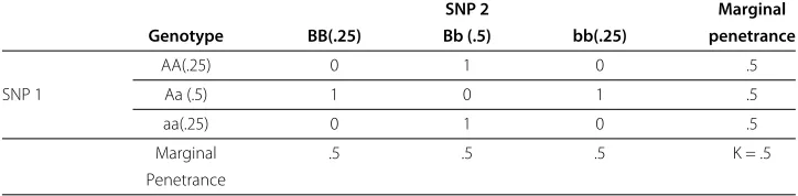
Table 1 Penetrance function providing penetrance values for three genotypes from a SNP acting under an autosomal recessive disease model
SNP 1
AA(.25) Aa (.5) aa(.25)
0 0 1
Genotype frequencies are given in parenthesis andq=p=.5.
This penetrance function isfully penetrant, since disease status is completely dependent on genotype (i.e. penetrance values are either 0 or 1). For single-locus models such as this, one can quickly determine if the SNP displays any main effect. The absence of a main effect would manifest itself as equal penetrance values for all three genotypes. Penetrance functions are easily extended to describen-locus interactions betweennpredictive loci using a penetrance function comprised of 3npenetrance values corresponding to each of the 3nMLGs.
Statistical models of epistasis
We classify models of statistical epistasis intopureandimpure, as well asstrictandnested
subtypes. For each, we say thatnloci interact epistatically if the heritability of thenloci together exceeds the sum of the heritabilities of each of thenloci individually.Purerefers to epistasis betweennloci that do not display any main effects [8,26,30]. Alternatively, impure epistasis implies that one or more of the interacting loci have a main effect con-tributing to disease status (see §1.1 in Additional file 1).Impureepistasis should be easier for non-exhaustive data analysis strategies to detect since any main effect(s) could serve as a guide towards the correct multi-locus interaction.Strictrefers to epistasis wheren
loci are predictive of phenotype but no proper multi-locus subset of them are. By defini-tion, all 2-locus epistatic interactions are strict.Nestedrefers to epistasis in which at least one proper subset of the loci also interact epistatically. Nested epistasis should be easier for non-exhaustive data analysis strategies to detect since the nested subset of loci could serve as a guide towards the correctn-locus interaction. To the best of our knowledge, the
literature has yet to consider the distinction between strict and nested epistasis. Figure 1 illustrates the distinction betweenpure / impureandstrict / nested. The present study explores the generation of worst-case models of epistasis, that are both pure and strict. However, the methods we present can be easily extended to the other types of epistatic models just described.
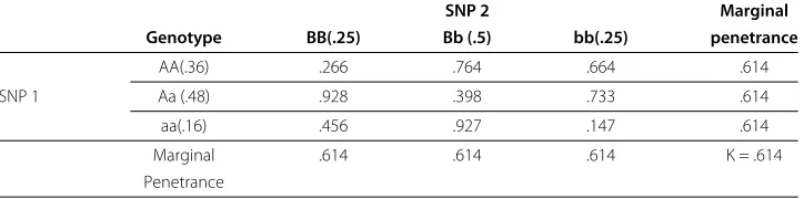
Tables 2 and 3 give examples of epistatic models that are both pure and strict. While fully penetrant models, like those found in Tables 1 and 2 are easy to interpret, they are rarely representative of real interactions. More realistic models, like the one in Table 3 and the ones typically generated by GAMETES, possess continuous penetrance values between 0 and 1. The models from Tables 2 and 3 include a penetrance function relating two SNPs to risk of disease. Each of the nine entries in these tables correspond to one of the nine possible MLGs combining SNPs 1 and 2. For instance, according to Table 2, subjects that have the MLG (AA-Bb) are certain to have disease and according to Table 3 subjects that have the MLG (aa-bb) have a 14.7% chance of having disease. What makes these penetrance functions purely epistatic is that while the genotypes of SNPs 1 and 2 are together predictive of disease status, neither is individually. Indeed, in the case of Table 3, if an individual has genotype AA and SNP 2’s genotype is ignored, the probability he has disease is
.25·.266+.5·.764+.25·.664=
.25, .5, .25 · .266, .764, .664 =.614 (1)
which is the marginal penetrance associated with genotype AA. (Computations are to three decimals places.) If he has genotype Aa, the probability of disease is
.25, .5, .25 · .928, .398, .733 =.614 (2)
and for genotype aa it’s
.25, .5, .25 · .456, .927, .147 =.614 . (3)
Thus, SNP 1’s genotype alone is not predictive of disease status. Similar computations (using the probabilities of SNP 1’s genotypes and the columns in Table 3) give the same value of .614 for the three marginal penetrances associated with SNP 2. Therefore, SNP 2 alone is also not predictive of disease status. The equality of all six of these marginal pen-etrances is the mathematical definition of strict, pure epistasis for 2-locus models. Their common value equals the population prevalence of disease (K). An expanded definition forn-locus models is given in Additional file 1 (§2.3). It essentially says that an(n)-locus model is strictly and purely epistastic if all of then3n−1dot products, analogous to the six just discussed, are equal.
Table 2 A fully penetrant 2-locus purely epistatic penetrance function
SNP 2 Marginal
Genotype BB(.25) Bb (.5) bb(.25) penetrance
AA(.25) 0 1 0 .5
SNP 1 Aa (.5) 1 0 1 .5
aa(.25) 0 1 0 .5
Marginal .5 .5 .5 K = .5
Table 3 A 2-locus purely epistatic penetrance function
SNP 2 Marginal
Genotype BB(.25) Bb (.5) bb(.25) penetrance
AA(.36) .266 .764 .664 .614
SNP 1 Aa (.48) .928 .398 .733 .614
aa(.16) .456 .927 .147 .614
Marginal .614 .614 .614 K = .614
Penetrance
The GAMETES algorithm
We first outline some of the main ideas GAMETES uses to generate random, pure, strict epistatic models. More detail is given in the following sections, and still more is in Additional file 1 (§2). A key part of the GAMETES algorithm is that certain choices of 2n entries of ann-way strict, pure epistatic penetrance table uniquely determine the rest of the table. Here we are assuming that the population prevalence is specified. For example, the four entries .764, .398, .733 and .456 of the penetrance table in Table 3 determine the remaining five entries via equations (1), (2) and (3), and the analogous equations involv-ing the columns of the table. So a first attempt to generate random penetrance tables might be to randomly vary these entries or even to randomly seed the four positions in the penetrance table they occupy. Two difficulties arise with this. One is that the mere choice of these positions—the ones that would be randomly seeded—biases the resulting penetrance tables (to have, for instance, high heritabilites). The other is that varying the values, even slightly, of the four chosen entries might not produce a penetrance table. For instance, if the entry .398 of the four chosen ones is changed to .37, then the entry just below it is forced to be greater than one.
This latter difficulty is addressed by working with what we call pre-penetrance tables. These are easily converted to strict, pure, epistatic penetrance tables and are essentially such tables with all marginal penetrances equal to zero. Pre-penetrance tables were used in a somewhat different context from ours in §8 of [5]. There, they arise as the difference between the 2-locus genotypic means of a quantitative trait and the linear model which best fits these means, and so show the wealth of epistatic models. They are our starting point for generating these models, primarily becauseall pre-penetrance tables, unlike strict, pure, epistatic penetrance tables, are easily described: each point ofR2n, Euclidean space of dimension 2n, corresponds to a uniquen-locus pre-penetrance table. So picking a random point inR2n (only a random direction is needed) determines a random pre-penetrance table. Converting this to a pre-penetrance table gives our notion of a random, strict, pure, epistatic penetrance table.
There is a catch here which gets back to the first difficulty: the one-to-one correspon-dence between points ofR2nand all pre-penetrance tables depends on the choice of the 2n positions that are randomly seeded. The GAMETES algorithm accounts for this by choosing these positions as randomly as is computationally feasible, as discussed in the next section.
We think of a variable as occupying each of these 2npositions—the ones which, when
seeded, determine all the entries of a pre-penetrance table. We call these 2n variables
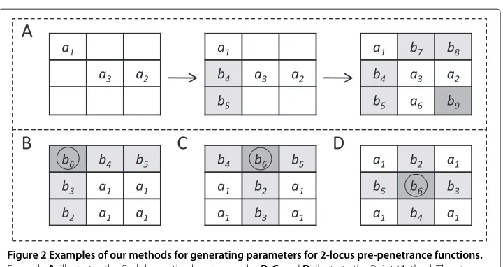
Figure 2 Examples of our methods for generating parameters for 2-locus pre-penetrance functions. ExampleA, illustrates the Sudoku method and examplesB,C, andDillustrate the Point Method. Thea’s (white boxes) are independent variables, or parameters, chosen by these two methods. Theb’s (grey boxes) are dependent variables, specified in terms of thea’s, where the dark grey boxes highlight the last variables to be specified. The subscripts indicate one of many orders in which these dependences can be found. In A, the variablesa1,a2anda3are first chosen by the Sudoku method, thenb4andb5are found in terms of these. After this, one of the four possibilities fora6is selected. The remainingb’s are then found. In B, C, and D, the circledb’s represent example reference points for the Point Method.
are possible for 2-locus tables. Parameters are independent variables for determining pre-penetrance tables since all entries can be expressed in terms of them.
Generating random parameters
A truly random way to pick parameters forn-locus pre-penetrance tables is to sequen-tially pick 2n positions at random and then check to see if these give parameters. The check, however, is computationally slow. (It requires determining if a 2n×2nmatrix is invertible.) Moreover, many such choices do not give parameters. GAMETES uses what we call the Sudoku method, a much more efficient approach to picking parameters, with only a slight loss of randomness (see Figure 2A). The Sudoku method also picks param-eters sequentially. However, after each choice, it expresses as many entries as possible in terms of the chosen parameters, and these are then omitted as possible future choices. This greatly reduces the number of choices which donot lead to parameters. Another advantage of the Sudoku method is that if after 2n choices all 3n entries of ann-locus table have been expressed in terms of the chosen ones, then no check is required: the 2n choices always give parameters in this case.
The Sudoku method always produces parameters randomly when the number of loci
nis 2. As ngrows, two things happen: (1) some bias occurs in parameter generation, and (2) the success rate for finding parameters decreases: forn = 2,. . ., 8, these rates were 100%, 99.9%, 99%, 92.9%, 61.2%, 3.28%, and 0% based on 750,000 GAMETES runs. Because of this, GAMETES uses what we call the Point method to generate parameters whenn≥6. Figure 2 (B,C,D) illustrates three iterations of the Point method in the case of two loci. Fornloci, the method starts by randomly choosing any one of the 3nentries. The
parameters the Point method then produces are the ones given by the 2nentries whose
From parameters to penetrance functions
Any pre-penetrance function can be converted to a pure, strict, epistatic penetrance func-tion by applying a linear scaling funcfunc-tionSto each of its entries. This functionSis defined by: theijthentry ofS(G),Gbeing any pre-penetrance function, isS(G)ij = gMij−−mm. Here
gij is theijthentry ofG, andMandmare the maximum and minimum respectively, of
the entries ofG. The entries ofS(G)lie in the interval [ 0, 1], with the minimum entry 0 and the maximum 1. Note that if all entries ofGare multiplied by any positive constantc, giving the pre-penetrance tablecG, thenS(cG)=S(G). So applying the functionSto all pre-penetrance tables in the direction ofG, meaning all positive multiples ofG, gives the same penetrance table.
Now, given a random direction of pre-penetrance tables, the functionSconverts it to our notion of a random, strict, pure, epistatic penetrance table. Choosing such a random direction requires an explicit description of all pre-penetrance tables. Any parameters, for instance those supplied by one of the methods discussed above, provide such a description. It takes the form of a one-to-one correspondence between all points of R2n
and all n-locus pre-penetrance tables. Specifically, given a point in R2n, the cor-responding pre-penetrance table has parameter values equal to the coordinates of the point. So, given randomly chosen parameters, picking a random direction of n-locus pre-penetrance tables now amounts to picking a random direction or, equivalently, a unit vector in R2n. We do this using G.W. Brown’s algorithm discussed on page 135 of [31].
Adjusting heritability and prevalence
Assume now that a random, pure, strict epistatic penetrance table with a specified her-itability, and perhaps also a specified prevalence is desired. Then GAMETES generates a random penetrance table as above and linearly scales its entries to achieve, if possible, the specified values. Linearly scaling the entries, meaning applying a function of the form
f(x)=mx+b,m>0 to each, changes the penetrance table in a relatively minor way so that randomness is preserved. If just heritability is specified, this scaling is done without changing prevalence. The required values ofmandbare discussed in Additional file 1 (§2.5).
Certain values of heritability and prevalence can never be achieved as discussed in the next section. So GAMETES will always fail if these values are specified. Also, penetrance tables with certain other values of heritability and prevalence are very sparse among all penetrance tables and so are generated by GAMETES with extremely low probability. For example, there existn-locus penetrance tables with all heritabilities≤1 having prevalence and all MAFs equal to 12. However, in both the 5 and 6-locus case, GAMETES generated none of these with heritability≥.1 after 100,000 iterations.
Limits on heritability and prevalence
The values of heritability and prevalence which a penetrance table can have are lim-ited. For instance, no penetrance table has heritability 1 and prevalence 14. The limits are more severe if MAFs are specified. For example, there are 2-locus penetrance tables with heritability 1 and prevalence12, but none if both MAFs are14. Penetrance tables with heritability 1 only exist if the MAFs are 12 or 1− √1
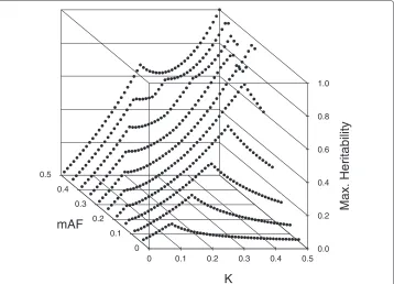
Culverhouse, et. al [26] summarized estimates of maximum heritabilities for 2 to 4-locus purely epistatic models over a range of MAFs and prevalence values. Figure 3 illustrates our maximum heritability estimates for pure, strict 2-locus epistatic models where both SNPs have the same MAF. Our method for estimating maximum heritabil-ity is discussed in Additional file 1 (§2.6). Generally speaking, if the prevalenceKis near .5, maximum heritabilities are largest when the MAFs are either 0.5 or 1− √1
2(≈ .29), and fall off as the MAFs move away from these values. For other values ofK, maximum heritabilities tend to increase with MAFs.
Summary of the GAMETES Algorithm
The GAMETES algorithm first (1) generates random parameters and a random unit vec-tor inR2n, then (2) generates a random pre-penetrance table by seeding these parameters using the unit vector, and then (3) uses the functionSto scale the entries of this random pre-penetrance table to generate a random penetrance table. In case a random penetrance table having a specified heritability, or heritability and prevalence is desired, it further (4) scales the entries of this penetrance table to achieve, if possible, these values. If the Sudoku method fails in step (1) or the scaling in step (4), the algorithm iterates until it either succeeds or a specified iteration limit is reached.
We give alternative descriptions, illustrated in Figure 4, of steps (2), (3) and (4) to clarify our notion of a random penetrance table. The parameters and vector given by successful completion of step (1) together determine a random direction of pre-penetrance tables. It consists of all pre-penetrance tables obtained by seeding the parameters with points in the direction of the vector. This random direction of pre-penetrance tables determines, in turn, a random class of strict, pure, epistatic penetrance tables. The members of this class consist of all penetrance functions which can be obtained from some pre-penetrance function in the random direction by linearly scaling its entries. These classes, one for each direction of pre-penetrance tables, partition the set of all strict, pure, epistatic penetrance tables. Each (successful) iteration of the GAMETES algorithm essentially picks, at ran-dom, one of these classes. The penetrance table in this class with maximum heritability
0 0.1 0.2 0.3 0.4 0.5 0
0.1 0.2 0.3 0.4 0.5
mAF
Max. Heritability
K
1.0
0.8
0.6
0.4
0.2
0.0
Figure 4 A schematic depiction of our method for picking random, strict, pure, epistatic penetrance functions.Points in the parameter space,R2ncorrespond to pre-penetrance functions, and points in the shaded region correspond to strict, pure, epistatic penetrance functions. The vectorVindicates a random direction in the set of pre-penetrance functions.Vdetermines a random class of penetrance functions, which is indicated by the line in the shaded region. The pointAon the boundary of this region indicates one (of the two) penetrance functions in this class with maximum heritability. The pointBindicates the penetrance function in this class having specified values of prevalence and heritability (if one exists). It may be viewed as random among all those with these values.
is our random penetrance table. In case a random, strict, pure epistatic penetrance table with specified values of heritability and prevalence is desired, GAMETES picks the unique (if any) penetrance table from this class with these values.
A GAMETES simulation study
of 200, 400, 800, and 1600 (400 datasets per model). For simplicity, each dataset was generated with a total of 20 SNPs. On whole we generated a total of 200 models and 80,000 datasets, all of which were evaluated using MDR.
For every evaluation, MDR was directed to search up to one order higher than the order of the simulated model. The best model was selected based on cross validation (CV) consistency, and in the event of a CV tie, based on testing accuracy. In this study, model detection success was evaluated, referring to the proportion of datasets within which the correct underlying model was identified. Detection success was considered to be meaningful when it was greater than 0.8.
Results and discussion
Table 4 gives the average run time required for GAMETES to make 100, 000 n -locus model generation attempts. Each average is based on 8 different runs of GAMETES in which pure, strict, epistatic models were sought with heritabilities of 0.005, 0.01, 0.025, 0.05, 0.1, 0.2, 0.3, or 0.4 (MAFs=0.5 and K=0.5). Run times were obtained running GAMETES on a 64-bit Dell PC with a 2.5GHz Intel Xeon Processor. The difference between run times for different heritabilities was negligible.
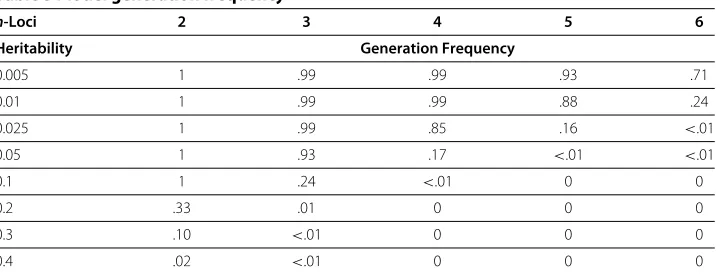
In addition to run time, we tracked the number of times a model was successfully generated having the specified set of model constraints. Table 5 indicates the frequency of successful model generation for each of the 8 specified heritabilities over alln-locus combinations explored. This frequency gives us an indication of how many iterations it takes to find a pure, strict, epistatic model with these specified heritabilities. As we approach the limits of what constraint combinations can be generated it takes GAMETES more attempts to successfully generate such models. In general, models of higher heri-tability take more attempts to find. This trend is exaggerated as the number of loci (n) is increased. The low likelihood of GAMETES to find models of high heritability is an expected limitation of the algorithm, since random models may only be scaled down to lower heritabilities during the model generation process.
In Additional file 1 (§3) we give the results of an example simulation study eval-uating MDR using the models and datasets generated with GAMETES as previ-ously described. We find that GAMETES is able to generate models useful for such evaluations, i.e. models with constraints at the boundary of what MDR is able to detect.
Conclusions
This study introduces GAMETES, a fast and reliable strategy for the generation of com-plex genetic models with random architectures. Specifically, we focus on the generation of pure, strict n-locus epistatic models (considered to be the most difficult to detect). The
Table 4 Averagen-locus run time of GAMETES
n-Loci 2 3 4 5 6
Time(sec.) 2.5 5.5 15.3 46.7 153.2
Table 5 Model generation frequency
n-Loci 2 3 4 5 6
Heritability Generation Frequency
0.005 1 .99 .99 .93 .71
0.01 1 .99 .99 .88 .24
0.025 1 .99 .85 .16 <.01
0.05 1 .93 .17 <.01 <.01
0.1 1 .24 <.01 0 0
0.2 .33 .01 0 0 0
0.3 .10 <.01 0 0 0
0.4 .02 <.01 0 0 0
(based on 100, 000 attempts).
benefits of our strategy include (1) speed; deterministic calculation of models makes our approach much faster than an EA approach, (2) randomness; models are generated using a strategy which seeks to maximize the randomness of model architecture, (3) the abil-ity to precisely specify genetic constraints, (4) the abilabil-ity to generate a large population of models from which to choose, and (5) the potential to combine the GAMETES mod-eling strategy with any data simulation strategy. An obvious limitation of this approach is the difficulty it has finding models of higher heritability. However, GAMETES is profi-cient at finding models with heritabilities typically used in evaluating and comparing new bioinformatic strategies.
While the probability is low that these types of ‘extreme’ epistatic interactions occur in biology by chance alone, we instead focus on the fact that they ‘can’ occur. With that in mind, our focus on pure strict epistasis is intended to promote the development of strategies that can accommodate even the most challenging relationships. In doing so, we make minimal assumptions about the true nature of biological interaction. Notably, the GAMETES strategy may be extended to produce impure epistatic models, as well as nested epistasic models, which are more likely to occur by chance. This extension will be a focus of future work.
The GAMETES software is open source and freely available for download. It offers an intuitive and flexible framework for the simulation of complex genetic models, and the option to generate simulated datasets from these models. This software offers both a graphical user interface, as well as command line accessibility to facilitate the quick gener-ation of a large simulated dataset archive. The GAMETES software along with a detailed users guide is included as Additional files 2 and 3, respectively.
Availability and requirements
• Project name:GAMETES
• Project home page:http://sourceforge.net/projects/gametes/files/ • Operating systems:Linux, Mac, PC
Additional files
Additional file 1: Supplemental Materials.Includes supplemental background, methods descriptions, and results. Supplemental figures included in this document.
Additional file 2: GAMETES Software Version 1.0 Beta.The graphical user interface for the GAMETES software. This software is open source and includes a User’s Guide.
Additional file 3: GAMETES User’s Guide Version 0.1.0 Beta.A reference guide for using the GAMETES software.
Abbreviations
SNP: Single nucleotide polymorphism; EA: Evolutionary Algorithm; GAMETES: Genetic Architecture Model Emulator for Testing and Evaluating Software; MLG: Multi-locus genotype; HWE: Hardy-Weinberg Equilibrium; MAF: Minor Allele Frequency; K: Population Prevalence; MDR: Multifactor Dimensionality Reduction.
Competing interests
The authors declare that they have no competing interests.
Author’s contributions
RU co-developed the methodology and software, carried out experiments, and co-wrote the manuscript. JK devolped the mathematical proofs, co-developed the methodology, and co-wrote the methods and supplemental material of the manuscript. NSA co-developed the computational methodology, and carried out the run-time experiment. TH carried out experiment determining maximum heritabilities and worked on respective figure. JF co-developed the software, and programmed the GAMETES GUI software. JH co-developed software. All authors read and approved the final manuscript.
Acknowledgements
We thank Joshua Payne, Davnah Urbach, Christian Darabos, Richard Cowper, Nadia Penrod, Dov Pechenick, and Qinxin Pan for their careful review of this paper. This work was supported by the William H. Neukom 1964 Institute for Computational Science at Dartmouth College along with NIH grants AI59694, LM009012, and LM010098.
Received: 24 April 2012 Accepted: 14 September 2012 Published: 1 October 2012
References
1. Shriner D, Vaughan L, Padilla M, et al.:Problems with genome-wide association studies.Science2007, 316(5833):1840c.
2. Eichler E, Flint J, Gibson G, Kong A, Leal S, Moore J, Nadeau J:Missing heritability and strategies for finding the underlying causes of complex disease.Nat Rev Genet2010,11(6):446–450.
3. Thornton-Wells T, Moore J, Haines J:Genetics, statistics and human disease: analytical retooling for complexity.TRENDS in Genetics2004,20(12):640–647.
4. Bateson W:Mendel’s Principles of Heredity.Cambridge University Press; 1909.
5. Fisher R:The Correlation Between Relatives on the Supposition of Mendelian Inheritance. .Trans R Soc of Edinburgh1918,52:399–433.
6. Cordell H:Epistasis: what it means, what it doesn’t mean, and statistical methods to detect it in humans. Human Mol Genet2002,11(20):2463.
7. McKinney B, Reif D, Ritchie M, Moore J:Machine learning for detecting gene-gene interactions: a review.Appl Bioinf2006,5(2):77–88.
8. Cordell H:Detecting gene–gene interactions that underlie human diseases.Nat Rev Genet2009,10(6):392–404. 9. Moore J, Asselbergs F, Williams S:Bioinformatics challenges for genome-wide association studies.
Bioinformatics2010,26(4):445.
10. Carlborg O, Andersson L, Kinghorn B:The use of a genetic algorithm for simultaneous mapping of multiple interacting quantitative trait loci.Genetics2003,155(4):2000.
11. Ploughman L, Boehnke M:Estimating the power of a proposed linkage study for a complex genetic trait.Am J Human Genet1989,44(4):543.
12. Weeks D, Ott J, Lathrop G:SLINK: a general simulation program for linkage analysis.Am J Hum Genet1990, 47(3):A204.
13. Bass M, Martin E, Mauser E:Pedigree generation for analysis of genetic linkage and association.InPacific Symposium on Biocomputing Hawaii. USA: World Scientific Pub Co Inc; 2004:93.
14. Schmidt M, Hauser E, Martin E, Schmidt S:Extension of the SIMLA package for generating pedigrees with complex inheritance patterns: environmental covariates, gene-gene and gene-environment interaction. Stat App Genet and Mol Biol2005,4:1133.
15. Lemire M:SUP: an extension to SLINK to allow a larger number of marker loci to be simulated in pedigrees conditional on trait values.BMC Genet2006,7:40.
16. Nothnagel M:Simulation of LD block-structured SNP haplotype data and its use for the analysis of case-control data by supervised learning methods.Am J Hum Genet2002,71(suppl 4):A2363.
18. Moore J, Hahn L, Ritchie M, Thornton T, White B:Routine discovery of complex genetic models using genetic algorithms.Appl Soft Comput2004,4:79–86.
19. Mailund T, Schierup M, Pedersen C, Mechlenborg P, Madsen J, Schauser L:CoaSim: a flexible environment for simulating genetic data under coalescent models.BMC Bioinf2005,6:252.
20. Dudek S, Motsinger A, Velez D, Williams S, Ritchie M:Data simulation software for whole-genome association and other studies in human genetics.InPacific Symposium on Biocomputing: Hawaii, USA; 2006,11:499–510. 21. Li C, Li M:GWAsimulator: a rapid whole-genome simulation program.Bioinformatics2008,24:140. 22. Li J, Chen Y:Generating samples for association studies based on HapMap data.BMC Bioinf2008,9:44. 23. Greene C, Himmelstein D, Moore J:A Model Free Method to Generate Human Genetics Datasets with Complex
Gene-Disease Relationships.Evol Comput, Machine Learning and Data Mining in Bioinformatics2010,6023:74–85. 24. Li W, Reich J:A Complete Enumeration and Classification of Two-Locus Disease Models.Human Heredity2000,
50(6):334–349.
25. Hallgrímsdóttir I, Yuster D:A complete classification of epistatic two-locus models.BMC Genet2008,9:17. 26. Culverhouse R, Suarez B, Lin J, Reich T:A perspective on epistasis: limits of models displaying no main effect.
Am J Human Genet2002,70(2):461–471.
27. Motzkin T, Ralffa H, Thompson G, Thrall R:The Double Description Method.In: Kuhn, HW, Tucker AW (eds) Contributions to theory of games1953,2:51–73.
28. Ritchie M, Hahn L, Roodi N, Bailey L, Dupont W, Parl F, Moore J:Multifactor-dimensionality reduction reveals high-order interactions among estrogen-metabolism genes in sporadic breast cancer.Am J Human Genet 2001,69:138–147.
29. Hartl D, Clark A, Clark A:Principles of population genetics. Sinauer associates Sunderland, MA; 1997.
30. Brodie III E:Why evolutionary genetics does not always add up. Epistasis and the evolutionary process; 2000, pp. 3–19. 31. Knuth D:The Art of Computer Programming 1: Fundamental Algorithms 2: Seminumerical Algorithms 3: Sorting and
Searching. MA: Addison-Wesley; 1968.
doi:10.1186/1756-0381-5-16
Cite this article as:Urbanowiczet al.:GAMETES: a fast, direct algorithm for generating pure, strict, epistatic models with random architectures.BioData Mining20125:16.
Submit your next manuscript to BioMed Central and take full advantage of:
• Convenient online submission
• Thorough peer review
• No space constraints or color figure charges
• Immediate publication on acceptance
• Inclusion in PubMed, CAS, Scopus and Google Scholar
• Research which is freely available for redistribution