www.atmos-meas-tech.net/3/1217/2010/ doi:10.5194/amt-3-1217-2010
© Author(s) 2010. CC Attribution 3.0 License.
Measurement
Techniques
Reference Quality Upper-Air Measurements: guidance for
developing GRUAN data products
F. J. Immler1, J. Dykema2, T. Gardiner3, D. N. Whiteman4, P. W. Thorne5,6, and H. V¨omel1 1Richard-Assmann-Observatorium, Deutscher Wetterdienst, Lindenberg, Germany
2School of Engineering and Applied Sciences, Harvard University, Cambridge, Massachusetts, USA 3Environmental Measurement Group, National Physical Laboratory, Teddington, UK
4Goddard Space Flight Center, NASA, Greenbelt, Maryland, USA 5Hadley Centre, Met Office, Exeter, UK
6Cooperative Insitute for Climate and Satellites, NOAA, Asheville, USA
Received: 29 January 2010 – Published in Atmos. Meas. Tech. Discuss.: 16 April 2010 Revised: 23 August 2010 – Accepted: 1 September 2010 – Published: 9 September 2010
Abstract. The accurate monitoring of climate change im-poses strict requirements upon observing systems, in partic-ular regarding measurement accuracy and long-term stability. Currently available data records of the essential climate vari-ables (temperature-T, geopotential-p, humidity-RH, wind, and cloud properties) in the upper-air generally fail to fulfil such requirements. This raises serious issues about the abil-ity to detect, quantify and understand recent climate changes and their causes. GCOS is currently implementing a Ref-erence Upper-Air Network (GRUAN) in order to fill this major void within the global observing system. As part of the GRUAN implementation plan we provide herein funda-mental guidelines for establishing and maintaining reference quality atmospheric observations which are based on prin-cipal concepts of metrology, in particular traceability. It is argued that the detailed analysis of the uncertainty budget of a measurement technique is the critical step for achieving this goal. As we will demonstrate with an example, detailed knowledge of the calibration procedures and data process-ing algorithms are required for determinprocess-ing the uncertainty of each individual data point. Of particular importance is the careful assessment of the uncertainties introduced by correc-tion schemes adjusting for systematic effects.
Correspondence to: F. Immler ([email protected])
1 Introduction
1218 F. Immler et al.: Upper-Air Reference Measurements systems). Therefore, the amount of available data is
increas-ing. Most, if not all, of these observations need to be cali-brated to a standard or the applied methods need to be vali-dated by comparison to an accepted reference. The reliability of these calibration or validation procedures over long peri-ods of time is of particular importance if these observations are to provide irrefutable, useful data series suitable for mon-itoring climate changes. However, the necessary reference data are often not available, leading to the unsatisfying situ-ation that a huge majority of observsitu-ations are not traceable to standards of the international system of units (SI) (Ohring et al., 2007, 2005). This means that separate datasets from different stations, observing platforms, and technologies are not directly comparable and therefore cannot necessarily be combined to give reliable long-term records. Central points for reference quality is the traceability of its calibration and the analysis of measurement uncertainty. In atmospheric sci-ence as well as in other disciplines the discussion of mea-surement uncertainty is not as common as it should be, of-ten leading to questionable interpretations and conclusions (Moldwin and Rose, 2009).
The purpose of this paper is to provide general guidelines for establishing reference upper-air measurements using both in situ and remote sensing instrumentation. We define the requirements an observation must fulfil in order to serve as a reference which can be used for calibrating or validating other observing systems, in particular, satellite instruments. The challenges associated with satisfying the requirements of reference quality are illustrated by a case study. Because the GCOS Reference Upper-Air Network (GRUAN) is en-visaged to be a small, albeit globally distributed, network of ground stations (Seidel et al., 2009) the focus is on ground-based instrumentation but the principles are more universally applicable.
Most of the observations obtained from the higher atmo-spheric layers are either retrieved from remote sensing or disposable balloon-borne sensors. To make either of these subject to a robust calibration is a big challenge. Our aim is to provide guidelines that maximize confidence, while still considering the constraints of implementation within a global operational network with a finite budget (in contrast to an ac-tive research project). As such, we aim to elucidate the theo-retical basis for the GRUAN and give some actual examples that demonstrate how upper-air reference observations using radiosondes are currently being made at various sites.
This paper provides a general definition of the term “ref-erence” as context for GRUAN observations. Beyond deliv-ering reference data for other observation systems, GRUAN aims to produce robust long-term upper-air climate records. This implies quantitative constraints on the measurement properties, in particular with respect to their accuracy and their temporal and spatial density. These issues will be con-sidered in other studies, both outside and within GRUAN as outlined in the GRUAN implementation plan (GCOS, 2009a). The following section gives some basic definitions
of the most important terminology used. It is complemented by a glossary at the end of the article. Section 3 describes in detail the steps that need to be taken to achieve reference quality measurements. Section 4 shows how these concepts can be realized in practice using temperature profiles from radiosonde as an example. Section 5 provides a summary.
2 Terminology
The formal terminology relating to measurements and uncer-tainties is set out in the International Vocabulary of Metrol-ogy (VIM) guidelines (JCGM, 2008). The following sections discuss the terms of particular relevance to upper air mea-surements.
2.1 Errors and uncertainty
Every measurement has imperfections that give rise to an er-ror in the result. As a consequence, a measurement is never a perfect indicator of the instantaneous state of the measured parameter. Traditionally, an error is viewed as having two components, a random and a systematic one. A random error is the result of stochastic variation of quantities that influ-ence the measurement and can never be completely avoided. However, its effect can be reduced by increasing the num-ber of observations, since, by definition, its expected value is zero.
uncertainties that are much smaller than those required for GRUAN, it illustrates a practical and convincing method for reducing systematic error.
Following the “Guide to the expression of uncertainty in measurement” (JCGM/WG 1, 2008, GUM hereafter) it is expected that the result of any measurement has been cor-rected for all known significant systematic effects and that every effort has been made to identify such effects. It is im-portant not only to correct for systematic effects but also to robustly ascertain and document the uncertainty of this cor-rection. Clearly, this level of knowledge of the systematic effects requires a detailed understanding of all aspects of the measurement. The lack of exact knowledge of the value of the measurand is characterized by a random variable, the un-certaintyU, which is evaluated from the uncertainties of all input quantities, including the uncertainties of all corrections that were applied for systematic effects. Provided that proper corrections have been made for all systematic effects, the expectation value (or ”expected value”) of uncertaintyU is zero. In this case, the uncertainty of the measurement result can therefore be expressed by one single value, the standard uncertaintyuwhich is the estimated standard deviation of the random variableU.
In practice, the only way it can be assumed that all sys-tematic effects have been properly corrected for is that mea-surements made by very different physical principles agree to each other within their independent uncertainties (that is, a statistically significant difference between them can be re-jected at the desired confidence level). So the use of inde-pendent measurement methods is needed to confirm that the systematic effects have been correctly compensated for and therefore provide the best estimate of the overall uncertainty in the measured variable.
The GUM considers Type A and B evaluation of standard uncertainty. Type A evaluation can be used if N independent observationsxiof the same quantity have been obtained. The
standard uncertaintyuof the mean is estimated by
u= v u u t
1 N (N−1)
N
X
i=1
(xi− ¯x)2 (1)
If no series ofNmeasurements are available, the uncertainty must be determined by other means than the statistical anal-ysis of series of observations. Any of those other means are referred to as “Type B evaluation” in the GUM.
Since it is virtually impossible to observe a variable in the atmosphere at the same location and same time through sev-eral independent observations, Type B evaluation will play a major role for determining the uncertainty of aerological data within GRUAN. Using Type B evaluation, the variance u2 or the standard uncertaintyuare evaluated by scientific judgment based on all of the available information on the possible variability ofx. According to the GUM, the pool of information may include:
– previous measurement data;
– experience with or general knowledge of the behaviour and properties of relevant materials and instruments; – manufacturer’s specifications;
– data provided in calibration and other certificates; – uncertainties assigned to reference data taken from
handbooks.
(JCGM/WG 1, 2008) In atmospheric profile measurements the uncertainty needs to be determined for each data point (at each altitude) individually. All sources of uncertainty should be summarized to an uncertainty budget. The total result-ing uncertaintyu(x)is calculated from independent sources of uncertaintiesu(vj)associated with the input variablevj
according to the rule of uncertainty propagation for uncorre-lated input quantities:
u(x)= v u u t
N
X
j=1 ∂f (v
1,..,vN)
∂vj
u(vj)
2
(2)
whenx=f (v1,..,vN)describes the functional relationship
between the final result and the input variables. 2.1.1 Uncertainty of multiple measurements
When measurement results are averaged over temporal or spatial ranges, the uncertaintyuaof the averagex¯is derived
from the uncertainties of the individual measurementsui by
applying Eq. (2) to the rule for calculating the mean. Since the partial derivative of ua with respect to each individual
measurementxiis 1/Nit follows:
ua=
1 N
v u u t
N
X
i=1
u2i (3)
This means that the uncertainty is reduced with 1/ √
N, by considering a larger set of individual observations. However, this holds only if the input variables (uncertainties) are un-correlated. When the most significant source of uncertainty is caused by a particular systematic effect, the individual un-certainties are highly correlated. In this case the uncertainty of a mean value over N data points is estimated by
ua=
1 N
N
X
i=1
ui (4)
If all ui were equal, Eq. (4) yields ua=ui indicating that
1220 F. Immler et al.: Upper-Air Reference Measurements If the total uncertainty of an average calculated from the
uncertainties of individual data points obtained from either Eqs. (3) or (4) is less than the statistical uncertainty of the mean calculated by Eq. (1), the variability of the measurand exceeds the accuracy and resolution of the measurement sys-tem. In this case, it is possible to distinguish between mea-surement uncertainty and variability. The variability can then be expressed as the standard deviation of the observed values xi by
σ= v u u t
1 N−1
N
X
i=1
(xi− ¯x)2 (5)
The statistical dispersion of the measured values are indica-tive of the character of the measurand, namely the natural variability in the space and time frame of the atmosphere un-der consiun-deration, if, and only if, the measurement uncer-tainty is less than the variability, i.e.ua< σ/
√
N orui< σ.
It is important to note that the uncertaintyua, correctly
eval-uated, always characterizes a property of the measuring sys-tem, not of the quantity being measured. Therefore, both valuesua andσ should be reported as significant
informa-tion when averages of individual measurements have been used to calculate the final result of a measurement.
2.2 Metrological traceability
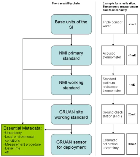
Metrological traceability is the property of a measurement re-sult whereby the rere-sult can be related to a reference through a documented, unbroken chain of calibrations, each of which contributes to the measurement uncertainty. Figure 1 shows the conceptual traceability chain for an upper air measure-ment, indicating the steps required to link the measurement to the fundamental SI units.Reference data are based on mea-surements that relate the measurands, i.e. the quantity to be measured, directly to a standard. This standard can either be an intrinsic standard (e.g., a reference standard that realizes a calibration scale based on a reproducible physical or chem-ical principle, such as a frostpoint hygrometer) or a certified reference standard (e.g., a standard that carries a calibration scale that is tied, according to a reproducible protocol, to a recognized community measurement standard). GRUAN stations should maintain a “GRUAN site working standard” for each basic unit, e.g. a thermometer periodically calibrated to a NMI standard (Fig. 1), that is used for calibrating the sensor for deployment. For example, in a pre-launch recali-bration procedure the thermometer of a radiosonde can be ad-justed to a thermometer with a certified calibration. These re-quirements establish traceability. Where the final data prod-uct of a reference observation depends on ancillary measure-ments, these measurements must again be traceable to stan-dards.
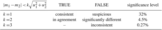
Table 1.Terminology for checking a pair of independent measurements of the same quantity for consistency.
|m1−m2|< k
p
u2
1+u22 TRUE FALSE significance level
k=1 consistent suspicious 32%
k=2 in agreement significantly different 4.5%
k=3 – inconsistent 0.27%
Fig. 1. Conceptual traceability chain illustrating how the calibration of a sensor for deployment is tied to the realization of a SI unit. Each calibration step is defined by a comparison between two measurements
with a stated, realistic uncertainty. All relevant details of the measurement comparison that can influence the
measurement result must be recorded.
SI: International System of units, from the French: Syste`me international d’unite´s
NMI: National Metrology Institute.
25
Fig. 1. Conceptual traceability chain illustrating how the
calibra-tion of a sensor for deployment is tied to the realizacalibra-tion of a SI unit. Each calibration step is defined by a comparison between two mea-surements with a stated, realistic uncertainty. All relevant details of the measurement comparison that can influence the measurement result must be recorded. SI: International System of units, from the French: Syste`me international d’unite´s. NMI: National Metrology Institute.
2.3 Measurement traceability
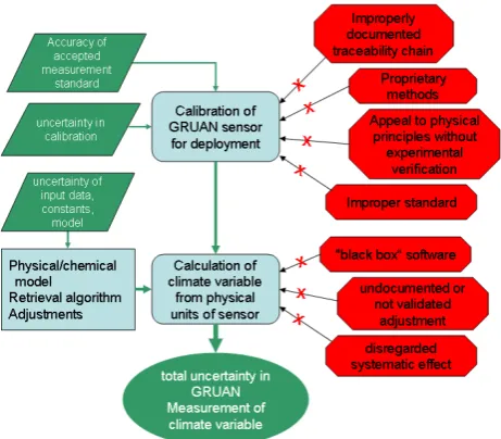
In particular, for climate research, it is important that data users have the opportunity to understand completely how the data that they are using for studying climate, were obtained. Therefore, every user should have access not only to the data, but also to a description of the instrument and algorithm used and, in particular, to any changes that occurred to either or both during the complete life cycle of the dataset (Fig. 2). Proper documentation of the measurements and all related metadata is essential.
2.4 Reference
Fig. 2. Schematic for establishing reference quality. Reference data must be traceable to an accepted
stan-dard. The red boxes contain components jeopardizing traceability. The procedure establishing traceability and
determining the uncertainty must be transparent and reproducible.
26
Fig. 2. Schematic for establishing reference quality. Reference data
must be traceable to an accepted standard. The red boxes contain components jeopardizing traceability. The procedure establishing traceability and determining the uncertainty must be transparent and reproducible.
measurement is that the uncertainty of the calibration and the measurement itself is carefully assessed. This includes the requirement that all known systematic errors are considered and corrected, and that the uncertainty of these corrections is determined and reported. An additional consideration for a reference measurement is that the measurement method and associated uncertainties should be accepted by the user com-munity as being appropriate to the application.
Another important requirement is that the methods by which the measurements are obtained and the data products calculated must be reproducible by any end user, at any time in the future. It should be kept in mind that these end users will continue to look at climate records for decades to come. They should be able to reproduce how measurements were made, which corrections were applied, and be informed as to what changes occurred during the observation and post-observation periods to the instruments and the algorithms.
In brief, reference within GRUAN means that, at a min-imum, the observed profiles are tied to a traceable standard at one point (e.g., by an extended, manufacturer-independent ground check of a radiosonde), that the uncertainty of the measurement (including corrections) is determined, and that the entire measurement procedure and set of processing al-gorithms are properly documented and accessible.
2.5 Redundancy and consistency
One important factor of GRUAN is that independent mea-surements of the same (or related) variables will be reported
in a consistent way. Traditionally, atmospheric observato-ries operate a large set of instruments, some of which mea-sure the same variable or related variables that strictly de-pend on each other (e.g., like water vapor profiles and total column water vapor). An important requirement of GRUAN will be that such redundant measurements are cross-checked for consistency as an essential part of the quality assurance procedures. Since all data are to be reported with uncertain-ties, a consistency check is, in principle, a straight forward task. Roughly speaking, consistency is achieved when the independent measurements agree to within their individual uncertainties.
Speaking in a mathematically more formal way, the hy-pothesis that two measurements have the same mean value should be tested by statistical methods at a given significance level. For the purpose of most GRUAN quality control tasks the Gaussian test (or “Z-test”) will be the most appropriate way to do this. It requires the knowledge of the measure-ments uncertainty. It is helpful to introduce the coverage fac-torkwhich determines an interval about the mean value as a multiple of the standard uncertainty. Based on the probability density function (PDF) of the dispersion of the uncertainty, the probability that values within this interval are measured can be calculated. Consider two independent measurements m1andm2of the same measurand with standard uncertain-tiesu1, and u2, respectively. Assuming that the hypothesis thatm1=m2is true and that the uncertainty is normally dis-tributed, the probability that
|m1−m2|> k· q
u21+u22 (6)
occurs only by chance, is roughly 4.5% fork=2 and 0.27% fork=3. Speaking in statistical terms, if Eq. (6) is true for k=2, the null hypothesis thatm1=m2can be rejected at a significance level of 4.5%. Simply speaking, it is very likely that the two measurements did in fact not measure the same thing, probably due to some unrecognised or unaccounted for systematic effect. We suggest to call data in this case “signif-icantly different” and if Eq. (6)holds fork=3 “inconsistent”. If the results agree withink=1 (i.e.|m1−m2|<
q
u21+u22) the data are “consistent”, and withink=2 they are “in (sta-tistical) agreement” (Table 1). Supporting the hypothesis m1=m2 the test loses statistical power with increasing k, while the confidence of correctly rejecting the hypothesis in-creases withk.1
The significance levels given in Table 1 can also be used to assess the quality of the uncertainty estimation: if large
1If Type A evaluation of uncertainty was used and both
mea-surement datasets have (about) the same standard deviations, it is more appropriate to use Students t-test for the consistency analysis with the significance levelsα=5% for defining “significant
differ-ence” andα=0.3% for defining “inconsistency”. However, since
1222 F. Immler et al.: Upper-Air Reference Measurements
Table 1. Terminology for checking a pair of independent measurements of the same quantity for consistency.
|m1−m2|< k
q
u21+u22 TRUE FALSE significance level
k=1 consistent suspicious 32%
k=2 in agreement significantly different 4.5%
k=3 – inconsistent 0.27%
sets of data are compared and a fraction much larger than 4.5% are significantly different, then either a systematic ef-fect on either or both measurements have been overlooked or the uncertainty was estimated too small. On the other hand, if much less than 32% of data are suspicious the measurement uncertainties are probably smaller than estimated.
If one of the two measurements does not provide uncer-tainties, the same methodology can still be used. The consis-tency analysis is made the same way by settingu2in Eq. 6 to zero(making the test statistically more powerful, i.e. the risk of yielding false confidence lower, than by arbitrarily as-signing some finite value tou2). This is equivalent with the notion that this value “does or does not lie within the error-bars with a specified coverage factor of the reference mea-surement”. If none of the measurements has uncertainties attached, a meaningful consistency analysis is not possible.
Problems arise from co-location and co-incidence issues (a radiosonde profile is never obtained at the same time and location as a ground-based or space-based total column measurement). These issues are considered by Seidel et al. (2010). The reader is referred to the GRUAN implementation plan (GCOS, 2009a), for a listing of these and other issues and the working Groups/task teams in charge of addressing them.
3 Establishing operational upper-air reference observa-tions
The establishment of upper-air reference observations on an operational basis consists of definition, execution and evalu-ation phases. First, the requirements for the measurements, which have been assembled through broad participation of the community, must be understood. Second, a review must be conducted to identify the most appropriate measurement technologies. Third, the performance of those technologies must be systematically evaluated. Additionally, validation, re-calibration, and archiving must be designed and imple-mented for an operational environment.
3.1 Defining requirements
The climate monitoring requirements for upper-air reference observations have been specified in GCOS (2007). They were derived mainly from the demands of potential users of GRUAN data. However, there will be inevitable
con-straints arising from technical and budgetary limitations of GRUAN stations, affecting the type and frequency of obser-vations. The GCOS Working Group on Atmospheric Refer-ence Observations (WG-ARO) also made recommendations on requirements for GRUAN reference radiosonde (GCOS, 2009b). There is an ongoing discussion on how to deal with the disparity that often exists between the desirable and the feasible. In a first step, GRUAN data are obtained with currently available and affordable equipment, provided they meet the basic requirements outlined in these guidelines which are a traceable calibration and a thorough analysis of the uncertainty. In a second step, efforts are made to reduce the uncertainties to comply with the requirements of GCOS-112 and to encourage new technologies where they cannot be so reduced. These items should be accomplished in the initial phase of GRUAN from 2009–2013. A detailed anal-ysis of the sources of uncertainty is the first, and often most important, step to improve the accuracy.
3.2 Reviewing existing instruments and choosing candidate(s)
A number of factors come into play in assessing the suitabil-ity of instrumentation for GRUAN. These factors include:
– Instrumental heritage: how long has a sensor been in use by the community and for what purpose; how sub-stantial is the body of literature documenting its perfor-mance and measurement uncertainty; how widely dis-tributed is the knowledge base that facilitates the sen-sor’s successful operation?
– Sustainability: are the cost of operation of the sensor and the demands of the sensor on personnel consistent with the resources allocated for GRUAN sites; are the demand and technology available to support the produc-tion and utilizaproduc-tion of the sensor for a meaningful period of time?
– Robustness of uncertainty: is the underlying accuracy claim for sensor and/or its data products strong; i.e. will it pass the scientific scrutiny and will it be useful for GRUAN science objectives?
It is not expected that all GRUAN sites will use identical instrumentation. The compatibility of instrumentation from site-to-site, as determined by intercomparison and laboratory calibration activities, will, however, play a major role in eval-uating the appropriateness of sensors on a case-by-case basis. 3.3 Identifying and quantifying sources of uncertainty The major step of obtaining a reference quality data prod-uct is the identification and quantification of measurement uncertainties. Doing this using a type A (statistical) ap-proach is a well established procedure. The identification and quantification of type B uncertainties in a way that is robust (e.g., likely to hold up to critical scientific inquiry) is a much more challenging project. Examples of success, relevant to GRUAN, are the efforts to establish a standard for total column ozone using Dobson spectrometers (Komhyr et al., 1989), and Keeling’s extremely reliable measurements of carbon dioxide mixing ratios Keeling (1998) which have been ongoing for more than half a century. Similar meth-ods have been employed in other areas of natural sciences and in the definition and maintenance of physical measure-ment units by the international community of national stan-dards laboratories. Some examples of this include the utiliza-tion of quantum electrical standards to diagnose the biases in standard voltages realized with electro-chemistry (Hartland, 1988), as well as the example of acoustic thermometry used to check contact thermometry described above. GRUAN can take advantage of these successes by utilizing multiple mea-surement methods for essential geophysical variables, based on different physical principles, and by working to encourage and make use of ongoing research of relevant measurement methods. Synergies with existing networks like the Net-work for the Detection of Atmospheric Composition Change (NDACC), which has a focus on remote sensing of the free atmosphere, can be particularly helpful in this respect.
Error sources in radiosonde measurements are thoroughly discussed in the CIMO Guide to Meteorological Instruments and Methods of Observation (WMO, 2006, chapter 12.8). For GRUAN data the uncertainty arising from those sources for the specific sensor in use must be readily quantified and reported. Attempts should be made to identify and quantify unknown sources of uncertainty.
Some sensors/measurement devices derive their calibra-tion from a pre-deployment comparison against an estab-lished reference. The results of these pre-deployment cali-brations need to be checked to maintain the integrity of the measurement. Additionally, the ageing of components and exposure to unfavorable environmental conditions (e.g. ex-tremes of temperature or humidity, chemical contamination) can cause calibration drifts, which necessitate a full recal-ibration. These pre-deployment procedures generally add contributions to the uncertainty budget. Other sources of un-certainty arise from systematic effects that affect the sensor during deployment. One example is the positive bias on
air-temperature measurement caused by solar radiation (Luers, 1990). This effect is generally corrected for operationally. However, there is limited knowledge about the actual param-eters that determine the magnitude of the bias (e.g. radiation and ventilation of the sensor). Additionally, the properties of the sensor (e.g. absorption coefficients) and the mathemati-cal model to determine the bias have their uncertainties. In many cases these adjustments are a black box process. The fi-nite sensor response time also causes bias when the dynamic value of the measurand is changing rapidly relatively to the response time of the sensor. This occurs for example in hu-midity measurements in the troposphere with radiosondes, where rapid changes from humid to dry layers and vice versa can occur during the ascent. The polymer sensors utilized in most radiosondes are comparatively slow, in particular at cold temperatures, giving rise to the so-called ’time-lag er-ror’ (Miloshevich et al., 2004). Again, this effect can be cor-rected but introduces additional uncertainty, e.g. due to lim-ited knowledge of the time-lag constant (which is a function of temperature). All these pieces of the puzzle need to be considered when determining the overall measurement un-certainty at each point of an upper-air profile.
3.4 Defining and validating a GRUAN data product The operational concept that describes measurement method, calibration, procedures, and algorithms, including those used for corrections and estimation of uncertainties, establishes a data product for GRUAN. Such a data product needs to be validated before implementation as a product of the GRUAN network.
The validation will be made using redundant measure-ments and testing for agreement as described in Sect. 2.5. Validation is first and foremost a validation of the uncertainty estimates. Agreement of two independent measurements, preferably based on different measurement principles, pro-vides a high degree of confidence that no significant system-atic effect was disregarded and uncertainties were not under-estimated. As a larger number of comparisons become avail-able, statistical analysis permits the uncertainty estimates to be evaluated further. Referring to the significance levels in-dicated in table 1, one can deduce that if the measurements agree (|m1−m2|<2·
q
1224 F. Immler et al.: Upper-Air Reference Measurements Laboratory tests and intercomparisons are fundamental
methods for establishing and confirming uncertainty esti-mates of data products. Laboratory tests provide an op-portunity to investigate in detail the performance of sen-sors under controlled conditions and to measure differences against certified references or other standards. Data from these experiments can be used to detect biases that may be corrected for and to determine calibration uncertainties. Field intercomparisons allow multiple in situ sensors and re-mote sensing data to be directly compared under the actual atmospheric conditions of the required measurement, and include all of the complex environmental conditions (tem-perature, humidity, pressure, wind/flow rate, radiation, and chemical composition) that cannot be fully reproduced in the laboratory. These complementary activities increase confi-dence that measurements are subject to neither unanticipated effects nor undiscovered systematic uncertainties. There-fore field experiments are particularly useful for validating GRUAN data products.
3.5 Implementing a GRUAN data product
From the required steps to develop a GRUAN data prod-uct described in the previous section, detailed procedures result. For a data product to be considered established and successfully validated, it needs to be documented in detail including a description of method, algorithms, and the in-field procedures for ensuring and controlling data quality. Results from validation experiments should be published in the peer-reviewed literature or technical notes with a strong preference toward the former. Once this is accomplished, and the data have been shown to meet the requirements of GRUAN regarding accuracy, operability, and stability the product can be considered for operational use at GRUAN sites and suitable for scientific applications. The description of the method and the measurement procedures will consti-tute an essential part of the GRUAN regulatory materials and procedures.
Implementation of a GRUAN data product at a site in-volves the installation of the required equipment and training of operators. Essential requirements for GRUAN operations are:
– pre-deployment recalibration to the GRUAN site work-ing standard,
– the routine collection of all relevant meta-data for mea-surements (e.g. reference values for recalibration, envi-ronmental conditions, etc.) and
– on-site quality assurance in general by consistency anal-ysis of redundant measurements.
The latter may be provided by the data processing facility or the Lead Centre.
The schedule of field recalibration and validation proce-dures should be drawn initially from experience with a given
sensor type, then refined according to the results of labora-tory tests and intercomparisons. The date and nature of field recalibrations should be included in metadata, so that if fu-ture experiments reveal shortcomings in schedules or meth-ods that were in use, uncertainty estimates can be adjusted after the fact to reflect those newly-discovered issues.
Other ways of assuring quality include comparisons to forecast data, visual inspection of curves by experienced staff, or consistency checks to physical principles. These checks do not generally feed directly into uncertainty bud-gets, but issues identified through such checks usually indi-cate problems with a specific measurement or unidentified systematic effects. Co-located in situ and remote sensing data are ideal for recurrent consistency analysis, provided that imperfect temporal and spatial co-incidence are consid-ered with respect to the variability of the measurand on the respective scales (Seidel et al., 2010).
3.6 Data archiving and processing issues
Designing proper data archive strategies is essential for es-tablishing a reference measurement network such as GRUAN that has as its over-riding aim long-term stability and trace-ability of its data products. Data at all intermediate stages of processing need to be archived, documented and dissemi-nated. Raw data (level 0) as produced by the instruments will generally be stored at the sites which need to ensure long-term availability of the data.
A first processing stage, essentially involving conversion to a common data format (e.g. NetCDF), produces level 1 data that will be archived at a dedicated central GRUAN facility. From raw data, a GRUAN data product (level 2) is derived by applying the necessary recalibrations, correc-tions, and the uncertainty analysis in a consistent and trace-able manner across identical instruments from different sites. This data, including its meta-data and documentation, must be easily accessible by end-users.
Data must be processed from one level to the next using algorithms that are fully documented and publicly accessible. Algorithm version control is crucial for this purpose. More details about proposed GRUAN data handling are described in the GRUAN implementation plan (GCOS, 2009a) and will be fleshed out in additional subsequent work.
and processed and able to reprocess as additional knowledge is accrued.
4 Example: determining uncertainty in radiosonde temperature profiles
In this section we give an example of how a reference quality measurement, in the sense described above, can be achieved for radiosonde temperature measurements using Vaisala RS92 or Graw DFM-06 radiosondes. This process is depicted schematically in Figs. 1 and 2. According to these figures, these steps include: substantiating the trace-ability of the temperature sensor calibration to the SI (in this case the ITS-90 temperature scale and thereby the Kelvin), evaluating the maintenance of that traceability through the ground check procedure, documenting and applying neces-sary corrections for systematic effects (particularly the radia-tion correcradia-tion), and critically assessing the final uncertainty achieved in the atmospheric temperature measurement. The most important step is the determination of the measurement uncertainty. There is ongoing research on these issues and the results discussed below should be considered prelimi-nary. A final assessment with more details will be the subject of a dedicated paper that is currently in preparation.
4.1 Requirements
The requirements for GRUAN measurements of tempera-ture have been specified in GCOS (2007), with an uncer-tainty of 0.1 and 0.2 K at a vertical resolution of 100 and 500 m in the troposphere and the stratosphere, respectively. Within the current state-of-the-art, these targets seem unre-alistic, since the perhaps most accurate temperature sonde, the “Accurate Temperature Measuring Radiosonde” (ATM) (Schmidlin, 1991), claims an uncertainty of 0.3 K throughout most of the upper troposphere and the stratosphere. How-ever, while maintaining the GCOS-112 specification as an ultimate goal for GRUAN, the current focus is on working out the steps described in Sects. 3.3 to 3.5 to establish a ref-erence network in the near future using the best measurement systems currently available.
4.2 Reviewing existing instruments
Instrument review is an ongoing process within the initial phase of GRUAN. It is not expected that all sites use identi-cal instrumentation. Establishing the uncertainty budgets of these instruments is an important step in ensuring the compa-rability of the measurements from different sites and identi-fying the technology that is best suited to fulfil the long-term goals of the network.
4.3 Establishing the uncertainty budget
4.3.1 Uncertainty arising from of the indication of the measuring system
The capacitive sensors of the RS92 or DFM-06 change the frequency of a resonant circuit depending on the sensor tem-perature. This frequency is of the order of 10 kHz and is measured and transmitted with a resolution of 0.01 Hz. The dependency of the frequency on temperature is roughly 0.5 Hz/K. The accuracy of the indication is therefore about 0.02 K and much lower than the stated uncertainty of the sen-sor of 0.15 K. It can be assumed that the contribution of the frequency measurement to the total uncertainty of the tem-perature sensor is negligible.
4.3.2 Calibration
The sensors of commercial radiosondes are generally cali-brated by the manufacturer who should be able to provide a certificate stating the uncertainty of calibration. If the cer-tificate is issued by a National Metrology Institute or an-other accredited agency, it generally ensures traceability to SI. A copy of the calibration certificate should be submit-ted to the GRUAN meta database. The accuracy of the cal-ibration is generally high, i.e., well below 0.1 K, through-out the entire temperature range under consideration (180 K to 310 K). The random error of the RS92 calibration (re-peatability) is 0.15 K (k=2) according to the 2005 brochure (Vaisala, 2006). The calibration uncertainty is considered to be an altitude-independent absolute systematic contribu-tion to the uncertainty profile. Altitude-dependent uncertain-ties are characterized separately. Some radiosondes are re-calibrated before launch by a ground check station – this is the case for the Vaisala RS92 radiosonde. This recalibra-tion needs to be handled with the same care as the manufac-turer’s calibration. The reference sensors of the ground check station should be regularly calibrated by a certified agency to ensure traceability to SI. In this case the reference sen-sor could be considered a “GRUAN site working standard” (Fig. 1).
The RS92 is recalibrated in a ground check station (GC25) where the sensor is put into a chamber equipped with two reference sensors (Pt 100). These references are supposed to be recalibrated with a cycle of two years. The Lindenberg GRUAN station holds a certificate (issued in 2009) indicat-ing “traceability to the National Institute of Standards and Technology” and states an uncertainty of 0.02 K.
1226 F. Immler et al.: Upper-Air Reference Measurements
Fig. 3.Correction of Vaisala RS92 radiosondes determined form the routine ground check.
27
Fig. 3. Correction of Vaisala RS92 radiosondes determined form
the routine ground check.
with a standard deviation of 0.2 K which was derived using Eq. (1). The reason why the mean value of these adjustments is larger than the claimed uncertainty of the calibration is not known and highlights the dangers of black box processes in ensuring the uncertainty chain (Fig. 2).
Here, the available knowledge about the calibration may not be sufficient to determine the uncertainty in a traceable way. We suppose the overall uncertainty of the calibration is better than 0.2 K but we have to use this number as long as we do not have direct evidence to support a lower uncertainty.
The temperature sensor of the Graw DFM-06 Radiosonde is calibrated in a chamber by the manufacturer to a standard that is traceable to SI. According to the calibration certifi-cate, uncertainty of the references, given here with a 95% coverage probability (i.e. k=2), is better than 0.02 K. The calibration curve of the radiosonde temperature sensors is determined from 12 comparisons in the range from 193 K to 303 K. The calibration curve is a polynomial least-square fit of degree 5 with differences to the measurement less than 0.015 K. Additional errors can arise from the compensation for temperature effects during flight which is obtained using “reference capacities”. This part of the measuring system is not included in the calibration but only in the in-flight mea-surement. Its contribution to the uncertainty is currently not known. The manufacturer GRAW specifies the total uncer-tainty of the temperature sensor of the DFM-06 with 0.2 K. Tests at the Lindenberg Observatory showed that the differ-ence between the DFM-06 sensor and a referdiffer-ence thermome-ter in a ventilated chamber is below 0.1 K, suggesting that the integration of the sensor in the radiosonde does not sig-nificantly change the calibration. Upon request, GRAW dis-closed the certificate of their calibration reference, a sample of a calibration protocol of an individual radiosonde sensor,
the algorithms used for calculating the temperature from the measured frequencies at the thermocapacitor, and the radia-tion correcradia-tion scheme that is applied. Raw data are stored during the radiosounding and are easily accessible. The mea-surement chain of this sensor is completely retraceable. 4.3.3 Radiation correction
The largest part of the overall uncertainty arises from the ra-diation that is absorbed or emitted by the sensor, in particu-lar during day-time measurements. Radiation can affect the measurement in different ways:
– Incoming radiation heats the sensor directly
– Indirect radiative heating: Incoming radiation heats the sensor framework, the mount that surrounds the ra-diosonde or any other part of the sounding equipment (incl. the balloon). This heat can then reach the sensor by conduction or via air passing over this part, warming up and then passing over the temperature sensor. – The sensor emits (long-wave) radiation and is thereby
cooled. This effect plays a significant role for sen-sors with white coatings, but is considered negligible for metallic coatings as used for the RS92 and DFM-06 (WMO, 2006).
Generally, a radiation correction is applied to the tempera-ture by the software in the receiving station. This correction should be documented in the accessible literature and de-pends on pressure, ventilation (ascent rate), and the incoming solar radiation. The latter is often parameterized using only the solar zenith angle (SZA). However, it depends on many more parameters, in particular the ground albedo, aerosols and clouds.
To assess the magnitude of the direct radiation correction several steps need to be taken:
the radiation correction CR (p, SZA) provided by the man-ufacturer needs to be validated by experiment. The Richard-Assmann-Observatory (RAO) in Lindenberg has recently measured the effect of direct radiation on the Vaisala RS92, InterMet 1, and Graw DFM-06 radiosonde. The details of these measurements will be published in a separate paper. A formula can be derived that relates the radiation effect to pressure, ventilation and incoming radiation.
Fig. 4.Total radiative field (actinic flux) derived from a radiative transfer model (streamer) for a November day
at noon at Lindenberg (52.21◦N, 14.12◦E) for a scenario without clouds (green) and with strong cirrus and
stratocumulus cloud layers (red) as a function of altitude. The blue curve shows the pdf of observed ground
total radiation ( (direct and diffuse)×(1+ground albedo) ) derived from 10 years of (BSRN) measurements in
November between 11:00 to 12:00 UTC (arb.units).
28
Fig. 4. Total radiative field (actinic flux) derived from a radiative
transfer model (streamer) for a November day at noon at Lindenberg (52.21◦N, 14.12◦E) for a scenario without clouds (green) and with strong cirrus and stratocumulus cloud layers (red) as a function of altitude. The blue curve shows the pdf of observed ground total radiation ( (direct and diffuse)×(1+ground albedo) ) derived from 10 years of (BSRN) measurements in November between 11:00 to 12:00 UTC (arb.units).
Lindenberg BSRN station during the period 1997–2006, the probability density function (PDF) of November noon actinic fluxes is shown in blue in Fig. 4. Roughly 90% of the mea-sured fluxes lie between the ground values of the modeled fluxes. Therefore, one may roughly assume that, with a cov-erage factor ofk=2, the radiation field lies within the ranges outlined by the red and green line. The uncertainty that this variability implies for the temperature measurement is shown in Fig. 5.
The problem with this assessment is that it is not based on the correction scheme applied by the radiosonde software because this scheme has not been disclosed by the manufac-turer. For a consistent uncertainty analysis it is imperative that the algorithms used for the correction be publicly avail-able.
4.3.4 Other sources of uncertainty
The effect of radiative balloon heating or adiabatic balloon cooling on the temperature data is considered to be negligible by the CIMO guide, provided the rope between balloon and sonde is at least 40 m (WMO, 2006, chapter 12.7.4.).
Fig. 5. Uncertainty derived for RS92 temperature profiles based on the considerations in the text: calibration
uncertainty (blue) and the uncertainty of the radiation correction (black) for November with a solar zenith
angle of 68◦. The total uncertainty is shown in red. Since both uncertainties are not correlated they are added
geometrically (Eq. 2).
29
Fig. 5. Uncertainty derived for RS92 temperature profiles based on
the considerations in the text: calibration uncertainty (blue) and the uncertainty of the radiation correction (black) for November with a solar zenith angle of 68◦. The total uncertainty is shown in red. Since both uncertainties are not correlated they are added geomet-rically (Eq. 2).
When the radiosonde emerges into dryer air above a cloud, evaporation of the condensed water cools the sensor and cre-ates a cool bias in this region (wetbulb effect). The RS92 seems to be less affected than other sensors, but, this effect can lead to deviations up to 1 K above a cloud and the data need to be flagged appropriately, e.g., by assigning a corre-spondingly increased uncertainty to data in such regions.
Another issue is the time-lag bias that was mentioned in Sect. 3.3. The time-lag of the temperature sensor of the RS92 is of the order of less then a second over the entire tempera-ture range (Vaisala, 2007). The temperatempera-ture during the ascent varies generally by less than a tenth of a degree in this time frame (along an adiabatic profile at a typical balloon ascent speed of 5 m/s the temperature gradient is 0.04 K/s). There-fore, it may be assumed that the bias caused by the time lag of the temperature sensor can be neglected.
4.4 Validating the temperature measurements
1228 F. Immler et al.: Upper-Air Reference Measurements
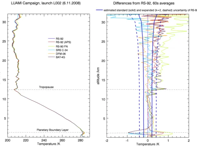
Fig. 6. Temperature profiles from radiosondes (left) launch with one balloon (L002) on 5 November 2008
at 10:45 UT during the Lindenberg Upper-Air Method Intercomparison campaign (LUAMI). The right panel
shows the differences with respect to the Vaisala RS92. The thick blue lines show the estimated standard (solid)
and expanded (k=2, dashed) uncertainty of the Vaisala RS92 temperature measurements.
30
Fig. 6. Temperature profiles from radiosondes (left) launch with one balloon (L002) on 5 November 2008 at 10:45 UT during the Lindenberg
Upper-Air Method Intercomparison campaign (LUAMI). The right panel shows the differences with respect to the Vaisala RS92. The thick blue lines show the estimated standard (solid) and expanded (k=2, dashed) uncertainty of the Vaisala RS92 temperature measurements.
sensor with respect to RS92. The thick blue lines indicate the uncertainty of the RS92 derived in the previous section. In the troposphere, above the boundary layer, the differences lie within the estimated uncertainty, indicating consistency be-tween all instruments. An exception is the range at about 1–2 km where the balloon had passed through a water cloud causing a wetbulb effect.
In the stratosphere, the differences are in some cases larger than the calculated uncertainties. These discrepancies are clearly due to the radiation effect since it increases signifi-cantly above a thick cirrus layer which was present at about 11 km. Most likely, the differences between the Vaisala APS instrument (which has the same temperature sensor as the RS92) and the RS92 are due to the indirect radiation effect enhanced by the way this radiosonde was attached to the rig which was not ideal for accurate temperature measurements (the focus of this campaign, and the APS in particular, was on humidity)
In summary this comparison demonstrates, that the esti-mated uncertainties are consistent with measurements from other instruments in the troposphere and into the lower strato-sphere, where there is no wetbulb effect. In the stratosphere some instruments (RS-90 FN, Intermet BAT-4G) show sig-nificant differences to the RS92. This is most probably due to larger (direct or indirect) effects of solar radiation on these other sensors. It should be noted, that this was not a proper validation experiment since there was no reference
instru-ment available. It is quite possible that all sensors have biases that can not be revealed by this experiment.
4.5 Improved ground check for RS92
At Lindenberg, every routine radiosonde is tested in an iso-lated vessel that contains purified water and is slightly heated and ventilated to ensure that the relative humidity in the ves-sel is at 100%. Since June 2009 this routine check for the hu-midity sensor has also included a certified temperature sen-sor. This enables an independent check of the calibration to be routinely obtained. Initial results indicate that the temper-atures agree to better than 0.1 K. As discussed in Sect. 4.3, the calibration uncertainty is probably much smaller than the one estimated from the RS92 groundcheck calibration. By simply using an independent ground recalibration to a certi-fied reference this error (and hence the overall uncertainty) could be considerably reduced.
4.6 Data archiving issue
already corrected for the radiation effect. It is important to track the corrections schemes that are used by Vaisala which have for the first time very recently been made available on their web-site (www.vaisala.com) in support of GRUAN con-verting what was a black box process into one that is now transparent. These data products are produced by scripts that generally are individually installed at each station. In order to provide homogeneous data it is necessary to install a com-mon ’GRUAN’ script on all participating stations that pro-duces a common and well defined (with respect to the ap-plied corrections and filtering) temperature profile necessary for the processing of higher level GRUAN data.
5 Conclusions
A pathway is described for the establishment of reference quality in upper-air climate observations, beginning with the choice of an appropriate instrument and proceeding through data archiving and documentation issues. We conclude that the essential requirement for a reference measurement is that all aspects of the measurement uncertainty are carefully de-termined and documented. Reference measurements must be tracable to the definition of a SI unit or to an accepted standard. The data must be corrected for known systematic effects and the uncertainty budget of the measurement needs to be established, which includes the uncertainties associated with any applied corrections. The resulting data product must be validated with in-field inter-comparisons. The mathemat-ical tool to evaluate redundant measurements were briefly described and it is demonstrated that uncertainty estimates are vital for performing a meaningful analysis of co-located measurements and validating their error budgets.
Proper documentation and data archiving strategies allow the user of reference data to understand in detail how the measurement was calibrated, conducted, corrected and qual-ity controlled. A comprehensive set of meta-data, collected along with the measurements, are necessary to track artifi-cial effects in long-term records. There is never a guarantee that there are no unrecognized systematic effects or that all such effects are properly accounted for. Therefore, additional measures must be implemented in order to ensure long-term stability of climate records, in particular when it comes to instrumental changes at a site. This includes the necessity of the ability to reprocess entire data streams if new issues are found.
In an example we demonstrate how the determination of the uncertainty budget is obtained in the case of a tempera-ture profile measured with a radiosonde. Based on knowl-edge of the calibration accuracy, additional laboratory tests, and pre-deployment tests an estimate of the calibration un-certainty was derived. Additional contributions of the uncer-tainty budget arise from the application of a radiation cor-rection that is necessary for daytime soundings which are impacted by direct radiative heating. A preliminary
valida-tion was undertaken based upon results from an intercompar-ison campaign carried out in Lindenberg in 2008 (LUAMI). Clearly, given the demands of determining the uncertainty and its validation, there is ample work left to be done. How-ever, an altitudependent uncertainty profile has been de-rived that is deemed a reasonable representation of the un-certainty of this sensor for the specific environmental condi-tions.
The framework presented here provides guidelines for ob-taining reference quality measurements to be implemented in the framework of the GCOS Upper-Air Reference Net-work (GRUAN). GRUAN, which is also a pilot project of the WMO Integrated Global Observing System (WIGOS), aims to provide long-term climate records of essential upper-air variables that can also serve as reference data for the cali-bration and validation of other observing systems, including satellite-borne sensors. For this application the data quality requirements described above are particularly useful. How-ever, it should be noted that reference quality is just one in-gredient necessary for reaching the goals of GRUAN. Other issues concern the maintenance of long-term stability, and the scheduling and accuracy requirements of measurements with regards to the determination of trends.
Appendix A Glossary
Measurand Quantity intended to be measured.
Uncertainty Property of a measurement, characterizing the disper-sion of a set or distribution of quantity values for the measurand, obtained by available information. Where possible, this should be derived from an experimental evaluation but can also be an estimate based on other information.
Standard uncertainty Measurement uncertainty expressed as a standard deviation.
Coverage probability Probability that the set of true quantity values of a measurand is contained within a specified coverage interval.
Coverage factor Number larger than one by which a combined stan-dard measurement uncertainty is multiplied to obtain an expanded measurement uncertainty
Type A evaluation of uncer-tainty
Evaluation of a component of the measurement un-certainty by a statistical analysis of measured quan-tity values obtained under defined measurement con-ditions.
Type B evaluation of uncer-tainty
Evaluation of a component of the measurement un-certainty determined by means other than a Type A evaluation of measurement uncertainty.
Variability Standard deviation from the mean value of a variable in a given temporal or spatial range, not to be con-fused with the measurement uncertainty.
Accuracy Closeness of agreement between the result of a mea-surement and a true value of the measurand.
Reference standard Measurement standard designated for the calibration of other measurement standards for quantities of a given kind in a given organization or at a given location.
1230 F. Immler et al.: Upper-Air Reference Measurements Intrinsic standard Measurement standard based on a sufficiently stable
and reproducible property of a phenomenon or sub-stance. The quantity value of an intrinsic standard is assigned by consensus and does not need to be es-tablished by relating it to another measurement stan-dard of the same type. Its measurement uncertainty is determined by considering two components: (A) that associated with its consensus quantity value and (B) that associated with its construction, implementation and maintenance.
Metrological Traceability Property of a measurement result whereby the result can be related to a reference through a documented unbroken chain of calibrations each contributing to the measurement uncertainty.
Acknowledgements. We like to thank the members of the working
group for atmospheric reference observations (WG-ARO) for helpful feedback on our draft, in particular Chris Miller, John Nash, Bill Murray, Masatomo Fujiwara, Dian Seidel, Junhong Wang, and Stephan Bojinski. P. Thorne was supported by the Joint DECC and Defra Integrated Climate Programme – DECC/Defra (GA01101).
Edited by: M. Weber
References
EUMETSAT: EUMETSAT, http://www.eumetsat.int, last access: 13 April 2010, 2009.
GCOS: GCOS Reference Upper-Air Network (GRUAN): Justifica-tion, requirements, siting and instrumentation options, Tech.Doc. 112, WMO TD No.1379, http://www.wmo.int/pages/prog/gcos/ Publications/gcos-112.pdf, 2007.
GCOS: GRUAN Implementation Plan 2009–2013, Tech. Rep., 134, WMO TD No. 1506, http://www.wmo.int/pages/prog/gcos/ Publications/gcos-134.pdf, 2009a.
GCOS: Specifications for a Reference Radiosonde for the GCOS Reference Upper-Air Network (GRUAN), Tech. Rep. Doc. 6.2a (6.II.09), GCOS, 2009b.
Hartland, A.: Quantum standards for electrical units, Contemporary Physics, 29, 477–498, http://www.informaworld.com/10.1080/ 00107518808222603, 1988.
JCGM: International vocabulary of basic and general terms in metrology (VIM), Tech. Rep. JCGM 200:2008, International Bu-reau of Weights and Measures (BIPM), http://www.bipm.org/ utils/common/documents/jcgm/JCGM 200 2008.pdf, 2008.
JCGM/WG 1: Evaluation of measurement data Guide to
the expression of uncertainty in measurement, International Bureau of Weights and Measures/Bureau International des
Poids et Mesures, www.bipm.org/utils/common/documents/
jcgm/JCGM 100 2008 E.pdf, Working Group 1 of the Joint Committee for Guides in Metrology, 2008.
Keeling, C. D.: Rewards and Penalties of Monitoring the Earth, Annu. Rev. Energ. Env., 23, 25–82, doi:10.1146/annurev.energy. 23.1.25, 1998.
Key, J. and Schweiger, A. J.: Tools for atmospheric radiative trans-fer: Streamer and FluxNet, Computers and Geosciences, 24, 443–451, doi:10.1016/S0098-3004(97)00130-1, 1998.
Komhyr, W. D., Grass, R. D., and Leonard, R. K.: Dobson spec-trophotometer 83 – A standard for total ozone measurements, 1962–1987, J. Geophys. Res., 94, 9847–9861, doi:10.1029/ JD094iD07p09847, 1989.
Luers, J. K.: Estimating the temperature error of the radiosonde rod thermistor under different environments, J. of Atmos. Oceanic
Techn., 7, 882–895, doi:10.1175/1520-0426(1990)007h0882,
1990.
Miloshevich, L. M., Paukkunen, A., V¨omel, H., and Oltmans, S. J.: Development and Validation of a Time-Lag Correction for Vaisala Radiosonde Humidity Measurements, J. Atmos. Oceanic Techn., 21, 1305–1327, 2004.
Moldwin, M. B. and Rose, S.: Documenting Precision and Accu-racy in the Open Data Policy Era, Tech. rep., Eos, 2009. NOAA: NOAA/NESDIS, http://www.nesdis.noaa.gov/, last access:
13 April 2010, 2009.
Ohring, G., Wielicki, B., Spencer, R., Emery, B., and Datla, R.: Satellite Instrument Calibration for Measuring Global Climate Change: Report of a Workshop., B. Am. Meteorol. Soc., 86, 1303–1313, doi:10.1175/BAMS-86-9-1303, 2005.
Ohring, G., Tansock, J., Emery, W., Butler, J., Flynn, L., Weng, F., St. Germain, K., Wielicki, B., Cao, C., Goldberg, M., Xiong, J., Fraser, G., Kunkee, D., Winker, D., Miller, L., Ungar, S., Tobin, D., Anderson, J. G., Pollock, D., Shipley, S., Thurgood, A., Kopp, G., Ardanuy, P., and Stone, T.: Achieving Satellite Instrument Calibration for Climate Change, EOS Transactions, 88, 136–136, doi:10.1029/2007EO110015, 2007.
Ripple, D. C., Strouse, G. F., and Moldover, M. R.: Acoustic Ther-mometry Results from 271 to 552 K, Int. J. Thermophys., 28, 1789–1799, doi:10.1007/s10765-007-0255-2, 2007.
Schmidlin, F. J.: Derivation and application of temperature correc-tions for the United States radiosonde, in: Symposium on Mete-orological Observations and Instrumentations, 7th, New Orleans, LA, 14–18 January 1991, Preprints (A92-32051 12-47), Boston, MA, American Meteorological Society, 227–231, 1991. Seidel, D. J., Angell, J. K., Christy, J., Free, M., Klein, S. A.,
Lanzante, J. R., Mears, C., Parker, D., Schabel, M., Spencer, R., Sterin, A., Thorne, P., and Wentz, F.: Uncertainty in Sig-nals of Large-Scale Climate Variations in Radiosonde and Satel-lite Upper-Air Temperature Datasets, J. Climate, 17, 2225–2240,
doi:10.1175/1520-0442(2004)017h2225:, 2004.
Seidel, D. J., Berger, F. H., Diamond, H. J., Dykema, J., Goodrich, D., Immler, F., Murray, W., Peterson, T., Sisterson, D., Som-mer, M., Thorne, P., V¨omel, H., and Wang, J.: Reference Upper-Air Observations for Climate: Rationale, Progress, and Plans, B. Am. Meteorol. Soc., 90, 361369, doi:10.1175/2008BAMS2540. 1, 2009.
Seidel, D. J., Sun, B., Pettey, M., Reale, T., and Immler, F.: Spa-tial Representativeness of Radiosonde Observations from Bal-loon Drift Statistics, J. Geophys. Res., submitted, 2010. Thorne, P. W., Parker, D. E., Christy, J. R., and Mears,
C. A.: Uncertainties in climate trends: Lessons from Upper-Air Temperature Records., B. Am. Meteorol. Soc., 86, 1437– 1442, doi:10.1175/BAMS-86-10-1437, http://journals.ametsoc. org/doi/abs/10.1175/BAMS-86-10-1437, 2005.
Titchner, H. A., Thorne, P. W., McCarthy, M. P., Tett, S. F. B., Haimberger, L., and Parker, D. E.: Critically Reassessing Tropo-spheric Temperature Trends from Radiosondes Using Realistic Validation Experiments, J. Climate, 22, 465–485, 2009. Vaisala: Vaisala Radiosonde RS92-SGP, available at: www.vaisala.
Vaisala: Vaisala Radiosonde RS92 Measurement Accuracy, 2007. WMO: Guide to Meteorological Instruments and Methods
of Observation, World Meteorological Organization, 7th
edn., www.wmo.int/pages/prog/www/IMOP/publications/