M E T H O D O L O G Y
Open Access
Transition-transversion encoding and
genetic relationship metric in ReliefF
feature selection improves pathway
enrichment in GWAS
M. Arabnejad
1, B. A. Dawkins
2, W. S. Bush
3, B. C. White
1, A. R. Harkness
4and B. A. McKinney
1,2** Correspondence:brett-mckinney@ utulsa.edu
1Tandy School of Computer
Science, The University of Tulsa, 800 S. Tucker Dr, Tulsa, OK 74104, USA 2
Department of Mathematics, The University of Tulsa, Tulsa, OK 74104, USA
Full list of author information is available at the end of the article
Abstract
Background:ReliefF is a nearest-neighbor based feature selection algorithm that
efficiently detects variants that are important due to statistical interactions or epistasis. For categorical predictors, like genotypes, the standard metric used in ReliefF has been a simple (binary) mismatch difference. In this study, we develop new metrics of varying complexity that incorporate allele sharing, adjustment for allele frequency heterogeneity via the genetic relationship matrix (GRM), and physicochemical differences of variants via a new transition/transversion encoding.
Methods: We introduce a new two-dimensional transition/transversion genotype
encoding for ReliefF, and we implement three ReliefF attribute metrics: 1.) genotype mismatch (GM), which is the ReliefF standard, 2.) allele mismatch (AM), which accounts for heterozygous differences and has not been used previously in ReliefF, and 3.) the new transition/transversion metric. We incorporate these attribute metrics into the ReliefF nearest neighbor calculation with a Manhattan metric, and we introduce GRM as a new ReliefF nearest-neighbor metric to adjust for allele frequency heterogeneity.
Results: We apply ReliefF with each metric to a GWAS of major depressive
disorder and compare the detection of genes in pathways implicated in depression, including Axon Guidance, Neuronal System, and G Protein-Coupled Receptor Signaling. We also compare with detection by Random Forest and Lasso as well as random/null selection to assess pathway size bias.
Conclusions: Our results suggest that using more genetically motivated
encodings, such as transition/transversion, and metrics that adjust for allele frequency heterogeneity, such as GRM, lead to ReliefF attribute scores with improved pathway enrichment.
Keywords: Machine learning, Feature selection, Genome-wide association study
(GWAS), Genetic relationship matrix (GRM), Transition and transversion
Background
ReliefF is a nearest-neighbors feature selection algorithm that is known for its ability to identify statistical interactions in high dimensional data [1, 2]. Specifically, it has been shown to identify gene-gene interaction effects in simulated and real genome-wide associ-ation studies (GWAS) [2]. ReliefF uses what is called a“diff”function to determine nearest neighbors in the space of single nucleotide polymorphisms (SNPs) and to compute the importance of a SNP based on its ability to separate cases and controls in the SNP space.
While ReliefF analysis of GWAS data depends critically on its ability to measure the degree of dissimilarity between genotype states, the diff function used up to this point has been extremely simple. For example, the standard ReliefF genotype diff between two subjects is binary: the diff is 0 when the genotypes of the two subjects at a SNP are identical and 1 if their genotypes are not identical. The distance between a pair of subjects is obtained by summing the diff values in a city-block (Manhattan) metric across all SNPs. The binary nature of this standard diff is likely an oversimplification that misses informa-tion because there are degrees of difference between genotypes. In addiinforma-tion to a metric based on allele-sharing differences, we develop a transition/transversion (Ti/Tv) metric that accounts for physicochemical differences of nucleotides and a Genetic Relationship Matrix (GRM) [3] metric that accounts for allele frequency heterogeneity.
The main goal of the current study is to develop and compare combinations of met-rics between SNPs and subjects in ReliefF feature selection. We also compare with stat-istical learning feature selection methods Random Forest [4] and Lasso (least absolute shrinkage and selection operator) [5]. Lasso has been used in GWAS [6,7] but is para-metric and generally uses a strong independence assumption among features. Random Forest has also been applied to GWAS and has fewer constraints than regression, which is an advantage when a multivariate genetic architecture may be involved in disease susceptibility [8–10]. We previously used Random Forest and penalized logistic regression as methods for comparing epistasis detection in simulated data [11]. When genes interact and have no marginal effect, we found that Random Forest has limited power to detect gene-gene interactions in high dimensional data, which was confirmed in Ref. [12]. The diminished Random Forest importance scores for interacting variants is attributable to the independence assumption in the tree node-splitting criterion.
In the current study, we use enrichment of pathways related to major depressive disorder (MDD) to compare feature selection methods. Early GWAS studies of MDD had limited success at finding significant variants due to the contribution of many loci with small effect sizes as well as the heterogeneous characteristics of MDD and the complex interaction between genetic variation and environmental factors [13]. In re-cent studies, many small main effect loci have been identified through the accumulation of extremely large samples [14,15]. Identifying broad pools of regulating, modulating or inter-acting SNPs that confer risk for a target disorder is an important goal. For example, bipolar disorder (BD) may occur in a family in which there is a primary susceptibility gene, but the majority of BD may involve the interactions of multiple genes [16]. Detecting these inter-action effects with ReliefF may be improved by tailoring metrics to GWAS data.
We apply ReliefF using combinations of diffs and metrics with other statistical learning methods to 463 cases of MDD and 459 controls, and we test the top se-lected SNPs and their corresponding genes for overlap with biological pathways related to mental disorders. Our results suggest that using more genetically moti-vated metrics (allele sharing and Ti/Tv) and metrics that adjust for allelic hetero-geneity (standardization by allele frequency in GRM) lead to ReliefF scores that improve enrichment of biologically relevant pathways.
Methods
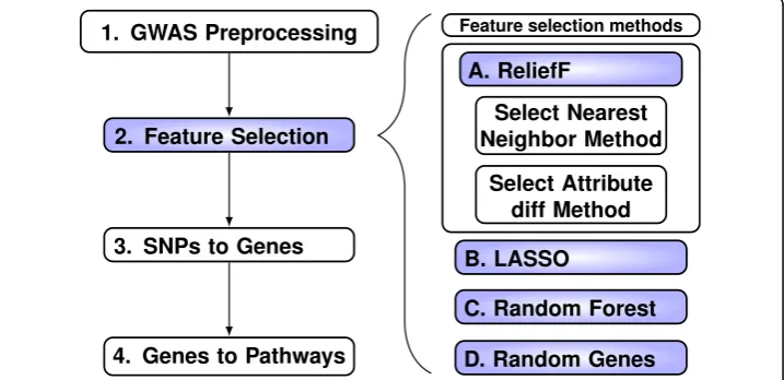
The goal of this study is to develop new ReliefF metrics for GWAS and compare them based on their ability to enrich for genes in pathways that have prior evidence for relevance to a phenotype. Our overall strategy (Fig. 1) is to compare enrich-ment of known relevant pathways. The analysis for each feature selection method involves four steps (left side Fig. 1). First we filter with minor allele threshold 0.01 and linkage-disequilibrium (LD) threshold 0.5 (Step 1, Fig. 1), which results in 281,648 SNPs prior to the application of each method. We choose the top SNPs from each feature selection method (Step 2) including ReliefF (Part A, Fig. 1), Lasso (Part B, Fig.1), Random Forest (Part C, Fig.1) and Random Genes of size 500 (Part D, Fig.1). The purpose of Random Genes is to estimate the effect of pathway size on enrichment due to chance. For each method, we choose the number of tops SNPs so that when we map SNPs to gene symbols (Step 3) we obtain 500 unique genes. Finally, we compare the number of genes detected for each of the biologically relevant pathways (Step 4).
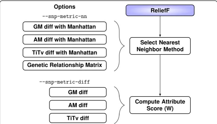
For ReliefF, we implement four methods for computing the nearest-neighbor distance matrix in our inbix software with --snp-metric-nn flag (Fig. 2) and three diff functions for computing the attribute importance score with --snp-metric-diff (Fig. 2). The three attribute importance diffs incorporate increasing nucleotide
information: binary genotype mismatch (GM), allele mismatch (AM), and transition/ transversion (Ti/Tv). Each of these diffs can be combined with a Manhattan metric to create three nearest neighbor methods. The Euclidean metric is also an option in our soft-ware. The last nearest-neighbor method is based on GRM. Each metric and diff function is discussed in detail below. We focus on six combinations: each of the three diffs used in the Manhattan metric for nearest neighbors and each of the three diffs used with GRM to compute nearest neighbors.
Relief feature selection algorithm
The goal of the Relief algorithm [17] is to estimate the importance of attributes accord-ing to how well their values distaccord-inguish between nearest neighbors from different clas-ses (e.g., caclas-ses and controls). The Relief algorithm uclas-ses a base “diff” function for the distance matrix to compute nearest neighbors, but the diff is also used for computing attribute importance. Recently we reformulated the ReliefF weight in a compact math-ematical form as a difference of means between nearest misses and hits [18]. A hit is defined for a given instance or subject Ri (i=1…m) as another instance that has the
same class label (case or control) as that of Ri, and a miss is another instance with a
different class label from Ri. Once a distance matrix, D, is computed between all
in-stances (discussed more below), the reformulated ReliefF score for SNP gν (ν =1…N) can be written as:
WR gν ¼Mgν−Hgν: ð1Þ
where the quantities
Mgν ¼mk1 X
m
i¼1
Xk
j¼1
diffgν;Ri;Mjð ÞRi : ð2Þ
and
Hgν ¼mk1 X
m
i¼1
Xk
j¼1
diffgν;Ri;Hjð ÞRi : ð3Þ
are the mean diffs with respect to SNPgνof all subjects Ri(i=1…m) from theirk
-near-est-neighbor misses [Mj(Ri) in Eq. (2)] and hits [Hj(Ri) in Eq. (3)]. The k nearest misses
for a subject Ri, are the k subjects nearest to Ribut in a different phenotype class than
Ri. Similarly, the set of hits of Riis the set of k subjects that are nearest to Riwhile
be-ing in the same phenotype class as subject Ri. An importance weight of SNPgν(WR[gν])
is higher if the average of the miss diffs for the instances is greater than the average hit diffs. Thus, a SNP with a greater positive value of WR(i.e,. Mgν >Hgν) is a better
pre-dictor of the phenotype because the genotypes of the SNP tend to separate instances in different classes more than instances in the same class. The diff function computes the amount that two genotypes are different for SNPgνbetween two subjects Riand Rj. In
the next subsection, we discuss in detail the new and old diff functions that will be compared.
New ReliefF diffs and metrics
We introduce three diff functions for measuring the genetic dissimilarity between pairs of individuals at a single locus. The first diff is the standard used in ReliefF for categorical variables, which we refer to as genotype mismatch (GM). The second metric accounts for allele sharing, which we refer to as allele mismatch (AM). The third diff further accounts for mutation type through transition/transversion differences (Ti/Tv). These first three diffs will be used to compute attribute importance and to compute city-block (Manhattan) distances between subjects. We will discuss these nearest-neighbor metrics and the genetic relationship matrix (GRM) in a later subsection.
Genotype mismatch
The standard metric used by ReliefF for categorical variables uses a binary mismatch diff. For SNPs, the genotype mismatch (GM) is a 0 or 1 difference between two individ-uals (R1,R2) for a SNP,gν, based on the individuals’genotypes. The diff function is
diffGM gν;R1;R2
¼ 0 ; genotype gν;R1
¼¼genotype gν;R2
1 ; otherwise
ð4Þ
where genotype(gν,R1) is the genotype for individualR1for SNPgν. In other words, two
individuals have zero diff if they have identical genotypes and they have unit diff if they have different genotypes.
Allele mismatch
difference in the number of alleles for a SNP when computing the difference between two individuals. The difference of two individuals can be calculated by the following formula
diffAM gν;R1;R2
¼1
2 jg1ν−g2νj ð5Þ
wheregiνis the number of copies of the reference allele for theνth SNP of theith
indi-vidual. In other words, the value ofg1νis the number of minor alleles in the genotype:
0, 1 or 2. Then the return value of diffAM(gν, R1, R2) is 0, 0.5 or 1 when the two
individ-ual have 2, 1 or 0 alleles in common, respectively.
Transition/transversion 2d encoding and associated diff
The AM diff increases the sensitivity over the GM diff because with AM a hetero-zygous state is half the distance between either homohetero-zygous state. Next our goal is to incorporate additional physicochemical information into the diff based on transi-tion and transversion mutatransi-tions. A transitransi-tion is a point mutatransi-tion (blue arrows in Fig. 3) that changes a purine nucleotide to another purine (A ↔ G) (orange circles in Fig. 3) or a pyrimidine nucleotide to another pyrimidine (C ↔ T) (green squares in Fig. 3). Transversion refers to the substitution of a purine (A or G) for a pyr-imidine (C or T) or vice versa (red arrows in Fig. 3) [19]. For the Ti/Tv diff func-tion, we classify genotypes as transitions or transversions and hypothesize that an allele mismatch at a transversion genotype is greater than the same mismatch for a transition genotype.
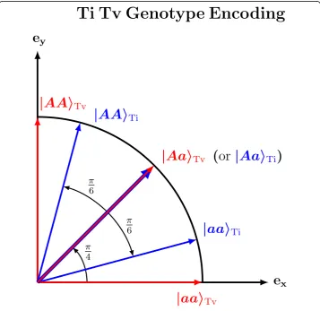
Before constructing the Ti/Tv diff, we first introduce a 2d Ti/Tv genotype encoding (Fig. 4) in which a genotype is a point on a unit circle in the Cartesian plane with basis vectors ex= (1, 0) andey= (0, 1). Below we use Dirac bra-ket notation, where |x〉
repre-sents a column vector and〈x| represents a row vector. An example of this encoding that is appropriate for transversion genotypes or an additive encoding (red arrows in Fig. 4) has the two homozygous states orthogonal (θ=π/2) to each other: |aa〉Tv=ex on the
horizontal axis and |AA〉Tv=eyon the vertical axis. And then the heterozygous state is an
equal mixture (θ=π/4) of the homozygous states:jAa〉Tv¼ ð1ffiffi 2 p ; 1ffiffi
2 pÞ.
For transition mutations, we want our encoding to contract the distance (relative to transversion encoding) between two homozygous states and between a homozygous state and the heterozygous state (blue arrows, Fig. 4). Again we let the heterozygous state bejAa〉Ti¼ ð1ffiffi
2 p ; 1ffiffi
2
p Þ, centered on the diagonal (θ=π/4) like transversions, but
in-stead of being orthogonal, the homozygous states are contracted toward the diagonal with an angle of separationθ=π/6.
Fig. 4Two-dimensional transition/transversion genotype encoding. Genotypes are represented as vectors on a unit circle and their similarity is the cos2θof their angular separation. Transversion genotype vectors
(red) are more expanded than transitions (byπ/4) to account for the alleles (A and a) coming from different nucleotide families (one purine and one pyrimidine). Transition genotype vectors (blue) are more
We use |ψi(gν)〉to represent the six possible 2d Ti/Tv genotypes (Fig.4) for
individ-ual Rifor SNPgν. The TiTv similarity between two individuals (R1and R2) for SNPgνis
the squared dot product of the individuals’Ti/Tv encoding (|ψ1(gν)〉and |ψ2(gν)〉):
simTiTv gν;R1;R2
¼ ψR1 gν jψR2 gν
2
¼ cos2ð Þθ12 ð6Þ
where hψR1ðgνÞjψR2ðgνÞi is Dirac notation for the dot product of the Ti/Tv genotype vectors and 〈ψR1ðgνÞj is the transpose of the column vector jψR1ðgνÞ〉. From Eq. (6), the diff can be written as
diffTiTv gν;R1;R2
¼1−simTiTv gν;R1;R2
ð7Þ
or
diffTiTv gν;R1;R2
¼1− ψR1 gν jψR2 gν
2
: ð8Þ
If gν is a transversion and individual R1 has homozygous genotype jψR1ðgνÞ〉
¼ jAA〉Tvand R2has heterozygous genotypejψR2ðgνÞ〉 ¼ jAa〉Tv, then the diff value is
diffTiTv gν∈Tv;R1;R2
¼1−hAAjAaiTv2¼1−ð0;1Þ∙ 1 ffiffiffi 2 p 1 ffiffiffi 2 p 0 B B @ 1 C C A 2
¼1−1
2¼
1
2:
For two individuals at a transversion SNP that are opposite homozygotes (jψR1ðgνÞ〉 ¼ jAA〉Tv and jψR2ðgνÞ〉 ¼ jaa〉Tv):
diffTiTv gν∈Tv;R1;R2
¼1−hAAjaaiTv2¼1−ð0;1Þ∙ 1 0
2¼1−0¼1:
Thus, the Ti/Tv diff for transversion SNPs is equivalent to AM because a heterozy-gous state is half the distance between either homozyheterozy-gous state.
Repeating the above examples for the transition encoding, the diff between jψR1 ðgνÞ〉 ¼ jAA〉Ti and jψR2ðgνÞ〉 ¼ jAa〉Ti is
diffTiTv gν∈Ti;R1;R2
¼1−hAAjAaiTi2¼1− 1=2;pffiffiffi3=2
∙ ffiffiffi 3 p =2
1=2
2¼1−3
4¼
1
4:
For individuals that are opposite homozygotes (jψR1ðgνÞ〉 ¼ jAA〉Ti and jψR2ðgνÞ〉 ¼ jaa〉Ti):
diffTiTv gν∈Ti;R1;R2
¼1−hAAjaaiTi2¼1− 1=2;pffiffiffi3=2
∙ 10
2¼1−1
4¼
3
4:
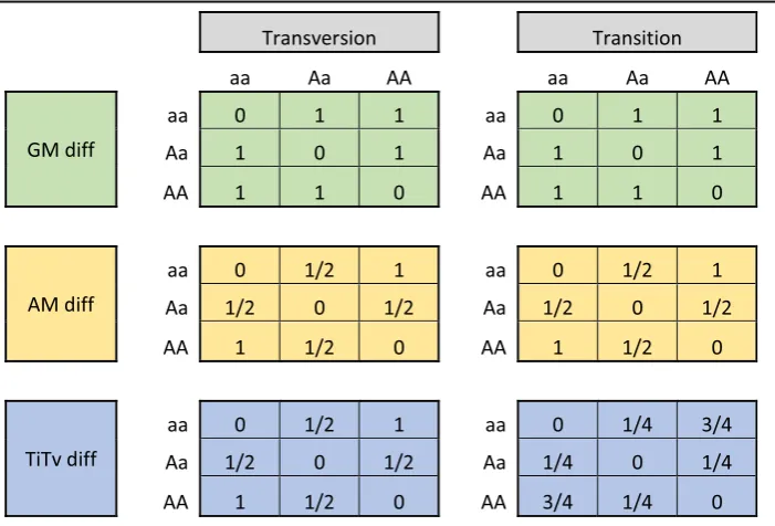
By design, this encoding causes the Ti homozygous diffs (3/4 difference) to be smaller than diffs between Tv homozygous states (1 difference) because transition mutations stay in the same biochemical family (purine to purine or pyrimidine to pyrimidine). Similarly, the encoding causes diffs between heterozygous and homozygous Ti geno-types (1/4 difference) to be smaller than the corresponding Tv diffs (1/2 difference).
difference (AA vs Aa) or (aa vs Aa). The AM diff (orange) is sensitive to allele differences between homozygotes (AA or aa) and heterozygotes (Aa), where the difference is 1/2 of the homozygous difference. However, AM does not distinguish between transition and transversion genotypes. The Ti/Tv diff (blue) is also sensitive to allele differences but further distinguishes between transition and transversion allele changes, treating transi-tion genotypes as more similar than the corresponding transversion genotypes. In this study, we focus on biallelic SNPs. The cases of tri-allelic and copy number variation may be interesting future modifications.
Nearest-neighbor distances based on Manhattan metric and the genetic relationship matrix (GRM)
We compare the above diffs (GM, AM, Ti/Tv) (Eqs.4,5,8) based on their influence in the attribute importance score (Eqs. 1–3). However, the diff may also be used to determine the distance between subjects by summing the absolute value of the diffs between a pair of subjects Riand Rjfor all genetic variantsgν(ν= 1…N) in a city-block
metric (Eq. 9 below). The standard ReliefF nearest-neighbor distance matrix for categorical variables uses the diff=diffGM(Eq.4) in the following metric:
Dcityij ¼X
N
ν¼1
diffgν;Ri;Rj
: ð9Þ
However, one may also replace diff=diffAM (Eq.5) or diff=diffTiTv (Eq. 8) in Eq. (9).
Regardless of the diff, when an attribute’s importance score is calculated, it uses the k Table 1.Comparison of the diff(gν,Ri,Rj) between individualsRiandRjfor SNPgνfor different
genotype combinations using GM (green, Eq.4), AM (orange, Eq.5), and Ti/Tv (blue, Eq.8) for all
combinations of genotypes and for the cases when the SNP is a transition or transversion
nearest neighbors as determined in the space of all other attributes, which allows ReliefF to identify important attributes that may involve complex higher-order inter-action architecture.
We also propose a more sophisticated metric for computing the nearest-neighbor dis-tance matrix based on the Genetic Relationship Matrix (GRM) from GCTA. The GRM is used to calculate the genetic relatedness between pairs of individuals in the space of N SNPs [3,20]. We define the following GRM distance matrix between individual i and j,
DGRM ij ¼
ffiffiffiffiffiffiffiffiffiffiffiffiffiffiffiffiffiffiffiffiffiffi
2N1−Aij
q
; ð10Þ
where
Aij¼N1 XN
ν¼1
giν−2pν
gjν−2pν
2pνð1−pνÞ ð11Þ
and giνis the number of copies of the reference allele for theνthSNP of theith
individ-ual andpνis the frequency of the reference allele [3]. Each genotype in the summand is
standardized by pνto account for the differences in allele frequency between SNPs. In addition to comparing diff functions (Eqs.4,5,8) in the attribute importance score, we also compare Manhattan (Eq. 9) and GRM (Eq. 10) methods for computing the pair-wise distances to find nearest neighbors.
Non Relief-based comparison methods: Random Forest, lasso, and random gene
Random Forests (RF) is a widely used machine learning classifier and feature selector that grows an ensemble of classification trees in bagged samples with random attribute selection [21]. To measure the importance of a feature after training, the values of that feature are permuted among the training data and the out-of-bag error is again com-puted on this perturbed data set. The importance score for the feature is comcom-puted by averaging the difference in out-of-bag error before and after the permutation over all trees and the score is normalized by the standard deviation of these differences [4,22–24]. We used the “Ranger” implementation of Random Forest, which is included in our inbix software to compute classification and variable importance.
We used the PLINK software to perform Lasso (--lasso). We adjusted for the first five principal components, and the PCs were not subject to model selection. The top Lasso variants were chosen by top regression coefficients. We used h2= 0.5 as the estimate of the heritability to calibrate the regression and we used λmin= 0.001 for the L1 penalty
parameter. Finally, we generated lists of random genes as a null comparison list that shows the effect of pathway size on enrichment. A random set of 500 genes is randomly sampled 100 times and the average overlap of the 500 genes is computed for each path-way. Estimating the expected number of overlapping genes by chance helps to calibrate the overlaps of each pathway for the non-random feature selection methods.
ReliefF software implementation
tool, written in C++ and designed to perform a range of large-scale analyses with compu-tational efficiency. The source is publicly available from our website and github (http://insilico.utulsa.edu/index.php/inbix/ and https://github.com/insilico/inbix) [18, 25,
26]. The inbix tool supports the PLINK format and includes PLINK algorithms and util-ities [27] along with new machine learning and network analysis methods. In our inbix software, we use the following command to execute ReliefF with a GWAS binary bed file <bed-file>.bed and a file containing phenotype information <pheno-file>.pheno:
./inbix --bfile <bed-file> --relieff --pheno <pheno-file> --snp-metric-nn <nn-metric> --snp-metric-diff <diff-metric> --out <results-file>
where <diff-metric> can take on values gm, am, or ti/tv and <nn-metric> can also take on values gm, am, or titv with manhattan or Euclidean for combining the individual SNP diffs. The user may alternatively select grm in <nn-metric>, which uses GRM as the nearest-neighbor metric and does not use the diffs. Any combination of <diff-metric> or <nn-<diff-metric> is allowed. For the MDD GWAS with 922 individuals and 281,648 SNPs (after filtering), the GRM metric takes approximately 8 hours and the other metrics take approximately 12 hours of CPU time (additional details in the Additional file1).
We use the constant-k ReliefF algorithm in inbix with the diffs and metrics described above. With inbix it is possible to optimize the number of neighbors for each attribute [18]. However, for this study, we use the constant value,k=⌊m/6⌋, for ReliefF nearest neighbors, where m is the number of samples. The valuek=⌊m/6⌋is the inbix default and was chosen based on Ref. [28] where it was shown to approximate the adaptive radius Relief method, MultiSURF [29], which balances power to detect epistatic effects and main effects.
GWAS data, filtering and mapping
In this study we compare ReliefF metrics with each other and with other analysis methods based on enrichment of selected features in functional pathways for MDD. We used a recent GWAS of MDD [30] that includes 922 European individuals that were recruited through a survey of 1259 individuals who filled out forms and telephone interviewed for DSM-IV covering depressive, bipolar, psychotic, alcohol, substance and anxiety disorders as well as family history of mood disorders. After exclusions, ex-tracted DNA was genotyped with the Illumina Omni1-Quad microarray for 463 cases of MDD and 459 controls. For all ReliefF analyses, we used constant k=⌊m/6⌋= 138 nearest neighbors.
Filtering and mapping of genes and pathways
A list of ranked SNPs for each method is obtained from the algorithms to be compared (Fig.1method overview). We use Ensembl IDs to map the top SNPs to genes [31]. Given the rs-number of a SNP, the algorithm finds the location of the variant relative to genes, and the SNP is mapped to the gene symbol of the closest gene [32]. In the supplement, we include a link to our webservice that accepts a list of SNP rs-numbers and returns mapped genes to a table, and we include the R code for the mapping. Despite LD pruning, many top SNPs will map to the same gene; thus, we begin the mapping with more than 500 top SNPs so that we end up with 500 top unique genes.
We then use Molecular Signatures Database (Msigdb) [33] to identify the number of genes in our top 500 gene selection lists that overlap with target pathways. The over-laps are based on HUGO gene symbols. Our goal is not to compute the statistical significance of overlap for discovery, but to compare the number of genes found in known pathways relative to other gene ranking methods. Thus, the size of the gene background is not a concern. We also use random gene selection, mentioned above, to show the expected amount of overlap with a pathway by chance.
Results
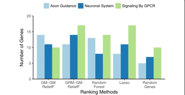
We evaluate feature selection methods based on the number of genes found in pathways that have been implicated in mood disorders (Figs.5,6and7). We chose pathways related to G protein-coupled receptors (GPCRs) because they are implicated in pathophysiology of MDD as well as bipolar disorder [34]. For example, current pharmacological interven-tions for MDD target neuromodulators (serotonin, norepinephrine, dopamine) that signal via GPCR systems. The other two pathways, Axon Guidance and Neuronal System, have been hypothesized to play an important role in mood disorder pathophysiology. In
0 5 10 15 20
GM−GM ReliefF
GRM−GM ReliefF
Random Forest
Lasso Random
Genes
Ranking Methods
Number of Genes
Axon Guidance Neuronal System Signaling By GPCR
0 5 10 15 20
AM−AM ReliefF
GRM−AM ReliefF
Random Forest
Lasso Random
Genes
Ranking Methods
Number of Genes
Axon Guidance Neuronal System Signaling By GPCR
Fig. 6Pathway detection comparison of AM-AM ReliefF and GRM-AM ReliefF. Bars count the number of genes that overlap the given pathway–Axon Guidance (light blue), Neuronal System (dark blue), and G protein-coupled receptor (GPCR) (green)–from the top 500 genes from each feature selection method. The methods are AM-AM (ReliefF with AM-based nearest neighbors (Eqs.5and9) and AM attribute diff (Eq.5)), GRM-AM (ReliefF with GRM-based nearest neighbors (Eq.10) and AM attribute diff (Eq.5)), where AM is allele mismatch and GRM is genetic relationship metric. In addition to ReliefF methods, we compare with Lasso with principal component covariates, Random Forest, and Random Genes (random sampling of 500 genes averaged over 100 replicates). AM-AM and AM have a similar pattern to and better performance than Random Forest. GRM-AM finds the most Axon and GPCR genes, and GRM-AM-GRM-AM finds the most Neuronal genes
0 5 10 15 20
TiTv−TiTv ReliefF
GRM−TiTv ReliefF
Random Forest
Lasso Random
Genes
Ranking Methods
Number of Genes
Axon Guidance Neuronal System Signaling By GPCR
Fig. 7Pathway detection comparison of TiTv-TiTv ReliefF and GRM-TiTv ReliefF. Bars count the number of genes that overlap the given pathway–Axon Guidance (light blue), Neuronal System (dark blue), and G protein-coupled receptor (GPCR) (green)–from the top 500 genes from each feature selection method. The methods are TiTv-TiTv (ReliefF with TiTv-based nearest neighbors (Eqs.8and9) and TiTv attribute diff (Eq.8)), GRM-TiTv (ReliefF with GRM-based nearest neighbors (Eq.10) and TITv attribute diff (Eq.8)), where TiTv is transition/transversion diff and GRM is genetic relationship metric. In addition to ReliefF methods, we compare with Lasso with principal component covariates, Random Forest, and Random Genes (random sampling of 500 genes averaged over 100 replicates). TiTv-TiTv has a similar pattern to but better
addition to ReliefF metrics, we compare with feature selection by Lasso, Random Forest, and the average of random gene selection to assess the number of genes expected by chance due to pathway size.
We compare combinations of ReliefF attribute diff functions for use in the average miss and hit calculations (Eqs.2and3) and metrics for computing nearest neighbors in the full space of SNPs. The diff functions are GM, AM, and Ti/Tv (Eqs.4,5, and8) and nearest neighbor metrics are the Manhattan metric (Eq.9) with the GM, AM and Ti/Tv diffs and the GRM metric (Eq.10). We compare the three combinations of <diff-metric> and two possible <nn-metric> for a total of 3x2=6 combinations (Figs. 5, 6 and7). We combine the three diffs with the same diff in a Manhattan metric to form the first three“ <nn-dif-f>-<attribute-diff>” combinations: GM-GM, AM-AM, TiTv-TiTv. We also combine the three diffs with GRM nearest-neighbor metric to form the other three“ <GRM-nn>-<attri-bute-diff>”combinations: GRM-GM, GRM-AM, GRM-TiTv.
We first note that for random gene selection (“Random Genes”on right-most side of Figs. 5, 6 and 7), the pathway overlap is correlated with the size of each pathway. As expected, choosing random genes will result in a certain amount of overlap with a pathway by chance in proportion to the size of the pathway. All methods perform bet-ter than chance (“Random Genes”) for detecting all pathways. For the Axon Guidance pathway, TiTv-TiTv (Eq. 8 for the Manhattan metric and attribute diff ) detected the most genes (light blue, Fig.7). For Signaling by GPCR pathway, GRM-TiTv (GRM near-est neighbor metric and TiTv attribute diff ) detected the most genes (green, Fig.7). For Neuronal System, GRM-GM performed best (dark blue, Fig.5).
Increasing in complexity of the diff (GM, AM, TiTv in Figs. 5, 6 and 7, respect-ively), shows pathway enrichment increasing when the attribute diff is used in the Manhattan metric (GM-GM < AM-AM < TiTv-TiTv). This suggests a benefit to including transition/transversion information in the attribute diff calculation for at-tribute importance. When the diffs are combined with GRM, the GPCR pathway enrichment increases significantly. The GRM metric adjusts for heterogeneity of allele frequencies, and detecting genes that contain SNPs with such heterogeneity likely benefits from GRM.
Discussion and conclusions
When testing for pairwise epistatic effects in a linear model, one may decompose the epistatic effects into additive and dominant encodings [36]. ReliefF has less flexibility to mix encodings than a pairwise-SNP linear model; however, ReliefF ranks SNPs within the context of all other SNPs in the dataset, which may include pairwise and higher-order interactions. In our approach, we are able to mix encodings in a given ReliefF analysis by using different diff functions for attribute importance (Eqs.1–3) and for finding nearest neighbors (Eqs. 9 or 10). The GM diff is based on a dominant single-locus encoding and the AM diff is based on an additive encoding. The Ti/Tv diff is based on a new 2d Ti/Tv encoding where a genotype is mapped onto a unit sphere and contracts transition genotypes closer together than corresponding transversion genotypes (Fig.4).
For each method, the top 500 SNPs were mapped to genes and overlap with the relevant biological pathways for major depressive disorder (MDD) was calculated. Our results provide evidence that using either AM (Eq.5) or Ti/Tv (Eq.8) diffs in the attri-bute importance score calculation (Eqs. 1–3) has an advantage over the simple GM diff (Eq.4). The detection of genes in certain pathways also can be improved by combining the attribute diffs with the GRM metric (Eq.10) for computing nearest neighbors.
The GRM method for finding nearest neighbors has the useful property of adjusting for alleleic heterogeneity. Using GRM to compute nearest neighbors results in the best enrich-ment for two of the three pathways: GPCR Signaling with GRM-TiTv (green, Fig.7, GRM nearest neighbor metric and TiTv attribute diff) and Neuronal System with GRM-GM (dark blue, Fig.5). The 2d TiTv encoding is the same as the AM diff for transversion SNPs but re-sults in genotype differences that are contracted closer together for transition SNPs. Using TiTv results in the best enrichment for the third pathway: Axon Guidance with TiTv-TiTv (light blue, Fig.7, TiTv used for the nearest neighbor metric diff and attribute diff).
We focused on the analysis of real data as a proof of principle. Additional insight may be obtained by using a simulation strategy that incorporates transition and trans-version differences that affect the phenotype. The challenge is to make such a simula-tion biologically realistic and not artificially biased toward one method. We used ReliefF’s simple nearest neighbor-finding method withk=⌊m/6⌋because it balances the ability to find main effect and interaction effects [28]. However, there are other Relief-based methods that may be used to optimize genetic findings. For example, one may use an adaptive attribute-specific number of neighbors to improve power to detect main effects and interaction effects [18]. One may also increase power through adaptive radius versions of Relief, like SURF [37], MultiSURF [29], and STIR [28], or through backwards elimination versions of Relief, like iterative ReliefF.
Additional file
Additional file 1:Command line details to use inbix to perform GWAS filtering and pathway enrichment and feature selection by random forest, lasso, and ReliefF with new transition-transversion diff and genetic relationship metric. (DOCX 35 kb)
Acknowledgements
Not applicable.
Funding
This work has been supported in part by The William K. Warren Foundation and the National Institute of General Medical Sciences Center Grants P20GM121312 and P20GM103456. The content is solely the responsibility of the authors and does not necessarily represent the official views of the National Institutes of Health.
Availability of data and materials
ReliefF and other methods used in this study are implemented in our command line bioinformatics tool called inbix (http://insilico.utulsa.edu/index.php/inbix/), which is written in C++ and publicly available from GitHub (https://github.com/insilico/inbix).
Author’s contributions
MA, BW, WB, AH, BD, and BM contributed to the design of the study. MA and BM wrote the manuscript. MA and BW performed analyses. All authors revised the manuscript critically for important intellectual content and approved the final manuscript.
Ethics approval and consent to participate
Not applicable.
Consent for publication
Not applicable.
Competing interests
The authors declare that they have no competing interest.
Publisher’s Note
Springer Nature remains neutral with regard to jurisdictional claims in published maps and institutional affiliations.
Author details
1Tandy School of Computer Science, The University of Tulsa, 800 S. Tucker Dr, Tulsa, OK 74104, USA.2Department of
Mathematics, The University of Tulsa, Tulsa, OK 74104, USA.3Institute for Computational Biology, Case Western Reserve University, 2103 Cornell Road, Cleveland, OH 44106, USA.4Department of Psychology, The University of Tulsa, Tulsa, OK 74104, USA.
Received: 8 July 2018 Accepted: 22 October 2018
References
1. Robnik-Šikonja M, Kononenko I. Theoretical and empirical analysis of ReliefF and RReliefF. Mach Learn. 2003;53:23–69. 2. Urbanowicz RJ, Meeker M, La Cava W, Olson RS, Moore JH. Relief-Based Feature Selection: Introduction and Review. J
Biomed Inform. 2018;85:189-203.https://doi.org/10.1016/j.jbi.2018.07.014.
3. Yang J, Lee SH, Goddard ME, Visscher PM. GCTA: a tool for genome-wide complex trait analysis. Am J Hum Genet. 2011; 88:76–82.
4. Breiman L. Random forests. Mach Learn. 2001:5–32.
5. Tibshirani R (2011) Regression shrinkage and selection via the lasso. J R Stat Soc Ser B (Statistical Methodol 73:273–282. 6. Jiang Y, He Y, Zhang H. Variable selection with prior information for generalized linear models via the prior LASSO
method. J Am Stat Assoc. 2016;111:355–76.
7. Wang H, Aragam B, Xing EP (2017) Variable selection in heterogeneous datasets: a truncated-rank sparse linear mixed model with applications to genome-wide association studies. In: 2017 IEEE Int. Conf Bioinforma Biomed. IEEE, pp 431–438.
8. Brieuc MSO, Ono K, Drinan DP, Naish KA. Integration of Random Forest with population-based outlier analyses provides insight on the genomic basis and evolution of run timing in Chinook salmon (Oncorhynchus tshawytscha). Mol Ecol. 2015;24:2729–46.
9. Stephan J, Stegle O, Beyer A. A random forest approach to capture genetic effects in the presence of population structure. Nat Commun. 2015;6:7432.
10. Li B, Zhang N, Wang Y-G, George AW, Reverter A, Li Y. Genomic prediction of breeding values using a subset of SNPs identified by three machine learning methods. Front Genet. 2018.https://doi.org/10.3389/fgene.2018.00237. 11. McKinney BA, Crowe JE, Guo J, Tian D. Capturing the spectrum of interaction effects in genetic association studies by
simulated evaporative cooling network analysis. PLoS Genet. 2009;5:e1000432.
13. Levinson DF, Mostafavi S, Milaneschi Y, Rivera M, Ripke S, Wray NR, Sullivan PF. Genetic studies of major depressive disorder: why are there no genome-wide association study findings and what can we do about it? Biol Psychiatry. 2014; 76:510–2.
14. Hyde CL, Nagle MW, Tian C, Chen X, Paciga SA, Wendland JR, Tung JY, Hinds DA, Perlis RH, Winslow AR. Identification of 15 genetic loci associated with risk of major depression in individuals of European descent. Nat Genet. 2016;48:1031–6. 15. Wray NR, Ripke S, Mattheisen M, et al. Genome-wide association analyses identify 44 risk variants and refine the genetic
architecture of major depression. Nat Genet. 2018;50:668–81.
16. Craddock N, Jones I. Genetics of bipolar disorder genetics of. bipolar disorder. 1999:585–94. 17. Kira K, L a R. A practical approach to feature selection. Proc Ninth Int Work Mach Learn. 1992:249–56.
18. McKinney BA, White BC, Grill DE, Li PW, Kennedy RB, Poland GA, Oberg AL. ReliefSeq: a gene-wise adaptive-K nearest-neighbor feature selection tool for finding gene-gene interactions and Main effects in mRNA-Seq gene expression data. PLoS One. 2013;8:e81527.
19. Collins DW, Jukes TH. Rates of transition and Transversion in coding sequences since the human-rodent divergence. Genomics. 1994;20:386–96.
20. Vrieze SI, McGue M, Miller MB, Hicks BM, Iacono WG. Three mutually informative ways to understand the genetic relationships among behavioral disinhibition, alcohol use, drug use, nicotine use/dependence, and their co-occurrence: twin biometry, GCTA, and genome-wide scoring. Behav Genet. 2013;43:97–107.
21. Chen CCM, Schwender H, Keith J, Nunkesser R, Mengersen K, Macrossan P. Methods for identifying SNP interactions: a review on variations of logic regression, random Forest and Bayesian logistic regression. IEEE/ACM Trans Comput Biol Bioinforma. 2011;8:1580–91.
22. Qi Y. Random Forest for bioinformatics. Ensemble Mach Learn. 2012:307–23.
23. Reif DM, Motsinger AA, McKinney BA, Crowe JE, Moore JH (2006) Feature selection using a random forests classifier for the integrated analysis of multiple data types. In: 2006 IEEE Symp. Comput. Intell. Bioinforma. Comput. Biol. IEEE, pp 1–8. 24. Meng YA, Yu Y, Cupples LA, Farrer LA, Lunetta KL. Performance of random forest when SNPs are in linkage
disequilibrium. BMC Bioinformatics. 2009;10(78).
25. Lareau CA, White BC, Oberg AL, Kennedy RB, Poland GA, McKinney BA. An interaction quantitative trait loci tool implicates epistatic functional variants in an apoptosis pathway in smallpox vaccine eQTL data. Genes Immun. 2016;17:244–50. 26. Davis NA, Lareau CA, White BC, Pandey A, Wiley G, Montgomery CG, Gaffney PM, McKinney BA. Encore: genetic
association interaction network centrality pipeline and application to SLE exome data. Genet Epidemiol. 2013;37:614–21. 27. Purcell S, Neale B, Todd-Brown K, et al. PLINK: a tool set for whole-genome association and population-based linkage
analyses. Am J Hum Genet. 2007;81:559–75.
28. Le TT, Urbanowicz RJ, Moore JH, McKinney BA. Statistical inference Relief (STIR) feature selection. Bioinformatics 2018 Sep. 2018:18.https://doi.org/10.1093/bioinformatics/bty788.
29. Granizo-Mackenzie D, Moore JH. Multiple threshold spatially uniform reliefF for the genetic analysis of complex human diseases. Lect Notes Comput Sci (including Subser Lect Notes Artif Intell Lect Notes Bioinformatics) 7833 LNCS. 2013:1–10. 30. Mostafavi S, Battle A, Zhu X, et al. Type I interferon signaling genes in recurrent major depression: increased expression
detected by whole-blood RNA sequencing. Mol Psychiatry. 2014;19:1267–74.
31. Zerbino DR, Achuthan P, Akanni W, et al. Ensembl 2018. Nucleic Acids Res. 2018;46:D754–61.
32. McLaren W, Pritchard B, Rios D, Chen Y, Flicek P, Cunningham F. Deriving the consequences of genomic variants with the Ensembl API and SNP effect predictor. Bioinformatics. 2010;26:2069–70.
33. Subramanian A, Tamayo P, Mootha VK, Mukherjee S, Ebert BL (2005) Gene set enrichment analysis : A knowledge-based approach for interpreting genome-wide.
34. Tomita H, Ziegler ME, Kim HB, et al. G protein-linked signaling pathways in bipolar and major depressive disorders. Front Genet. 2013;4:1–12.
35. Chang CC. Generalized iterative RELIEF for supervised distance metric learning. Pattern Recogn. 2010;43(8):2971–81. 36. Fish AE, Capra JA, Bush WS. Are interactions between cis-regulatory variants evidence for biological epistasis or
statistical artifacts? Am J Hum Genet. 2016;99:817–30.