Solar Tilt Angle Optimization of PV Systems for Different Case Studies

Solar Tilt Angle Optimization of PV Systems for

Different Case Studies

Hasan N. Muslim*

Department of Computer Techniques Engineering, Imam Al-Kadhum University College (IKUC), Najaf, Iraq.

Abstract

The evolution of solar photovoltaic systems (PV) in the last decade has been marvellous around the world. This growing in using of PV technique hinge on the electrical load profile that required to be covered and the rate of the electricity that can be generated from the areas where the solar cells to be installed. The production of PV systems is based on the fuel which is represented by the solar radiation. In this study, an algorithm has been proposed to optimize the solar tilt angle based on MATLAB software (m-file) in order to maximize the PV generation. Monthly and annually optimal tilt angles are suggested for different case studies those are: Najaf, California and New Delhi. Also, the estimation of solar radiation for each month is calculated according to their optimal tilt angles. The obtained results indicate that the yearly gain of solar radiation from orientation solar panels is approximately 18% for Najaf city and a high gain values for winter months with very small energy gains for summery months, and so on for other case studies. This proposed algorithm is general program and can be applied for any site on the earth by changing the latitude and longitude of the desired area.

Keywords: optimization, solar radiation, tilt angle, PV systems, solar cells, MATLAB. Received on 07 February 2019, accepted on 09 March 2019, published on 21 March 2019

Copyright © 2019 Hasan N. Muslim, licensed to EAI. This is an open access article distributed under the terms of the Creative Commons Attribution licence (http://creativecommons.org/licenses/by/3.0/), which permits unlimited use, distribution and reproduction in any medium so long as the original work is properly cited.

doi: 10.4108/eai.13-7-2018.157038

*_{Corresponding author. Email:[email protected]}

1. Introduction

Sun is the main source of the life on the earth and several phenomena and energies are created from it such as wind, rain, tide, biomass and hydroelectric energy, except geothermal and nuclear energy. Sun is the nearest star to the earth and lies in the centre of the solar group. Some of important specifications are illustrated in Table 1. [1].

The radiation that emitted from the sun is called solar radiation. It can be defined as the rate at which radiant energy is incident on a surface per unit area, and measured by W/m2_{. Solar cell is a device that converts the incident sun} light into electricity. The radiation reaching to the earth should be Fully benefited to produce the maximum energy from photovoltaic systems. Measured solar radiation data in the meteorological agencies are not accurate sometimes and has loss in data. Also, they measure the solar radiation on a horizontal surface not on optimized surface, and a long time is needed for optimization the solar tilt angle. Therefore, a perfect information of solar radiation availability at a particular geographic location is essential for the modelling

and designing of all solar thermal power stations and PV systems, architects, agriculturalists, air conditioning engineering and energy designing, atmospheric energy-balance, climatology, pollution studies, analysis of the thermal load on buildings, solar energy collecting systems and economic viability [2, 3].

Table 1. Main specifications of the sun [1].

Parameter Value

Total power on surface 3.84 * 1026 _W

Emission Power 6.3 * 107 _W/m2

Diameter 1.39 * 109 _m

Distance from earth 1.5 * 1011 _m

Mass 2 * 1030 _kg

Average temperature 5800 K

Hydrogen, helium, oxygen, carbon 71 %, 27 %, 0.97 %, 0.4 %

longitude, California in USA with 36.7782° N latitude and 119.4179° W longitude, New Delhi in India with 28.6448° N latitude and 77.2167° E longitude).

Number of previously published researches within optimization solar tilt angle and estimation solar radiation which are shown as follows. M. Benghanem, 2011, investigated the optimum choice of the tilt angle for the solar cells in order to collect the maximum solar insolation in Saudi Arabia depending on the measured values of daily diffuse and global solar radiation on a horizontal plane [4]. K. Bakirci, 2012, dealt with finding the optimum tilt angle of solar panels for solar energy systems using solar radiation data measured for eight big provinces in Turkey [5]. D. Lahjouji and H. Darhmaoui, 2013, examined the theoretical features that calculate the optimum tilt angle and makes recommendations on how to rise the solar energy collected by changing the tilt angle depending on the values of daily global radiation on a horizontal plane (from NASA) in Ifrane, Morocco [6]. T. Khatib, et al., 2015, presented an approach for optimizing the tilt angle of solar arrays installed in the five locations in Malaysia based on manually varying in tilt angle for maximum power generation [7]. A. K. Yadav and H. Malik, 2015, calculated the optimal tilt angle for six locations in India based on correlation in terms declination angle [8]. T. O. Kaddoura, et al., 2016, investigated optimum tilt angles of PV panels for different cities in the Saudi Arabia. Solar radiation data of horizontal surface for the study cities was obtained from NASA and MATLAB software was used in order to improve tilt angle [9]. N. Ihaddadence, et al., 2017, aimed to find the best inclination angle of fixed solar conversion systems in M'Sila region experimentally and theoretically (using empirical method) based on data taken from NASA Climatology resource for solar radiation on a horizontal surface [10]. A. A. Abbood, et al., 2017, suggested implementing energy management techniques using solar cells for residential sector in Baghdad city. The estimation of solar radiation data and PV system design has been simulated based on MATLAB software. The proposed tilt angles have been changed and optimized manually and based on conclusion for researchers [11]. Y. Lva, et al., 2018, an optimized mathematical model is proposed and used to calculate the optimal tilt angle and orientation of solar collectors set up in Lhasa during the summer season [12].

In this paper, an control method is proposed for optimizing tilt angle in the solar energy systems in order to maximize the PV generation. Matlab software based optimization for this purpose is used. The steps of the research are starting with illustration the theoretical background of solar radiation principles and concerned equations, then apply the suggested algorithm for different case studies with determining the monthly optimal tilt angles and calculating their solar insolation. This control technique is presented over the adaptive methods for controlling the tilt angle because the first one is most economic from the others that don’t need for using mechanical and electronic devices for optimizing inclination angle. Furthermore, the adaptive control methods require maintenance during the year and hence increasing the cost.

Also, it is difficult to use these devices in the large scale systems.

2. Solar radiation theory

Solar radiation or solar insolation can be defined as the beam produced or emitted by the sun measured in W/m2. The maximum amount of solar insolation reaches the surface of the earth is about 1000 W/m2 _{in a wavelength} limits from 0.3 μm to 2.5 μm as shortwave radiation which contains the visible spectrum [13]. Ignoring the reflection quantities, the hourly global solar insolation on a tilted surface in clear sky, Rt (W/m2) is given by the following

equation and as shown in Figure 1. [14],

(1)

Where,

Rn: Solar insolation on a plane that normal to the direction of

propagation.

Rb: Geometric factor which denotes the ratio of radiation

beam on the tilted surface to that on a horizontal plane at any time.

Rh: Solar insolation on a horizontal surface. θ: Incident angle on a tilted surface.

θz: incident angle on a horizontal surface.

Figure 1. Solar radiation on a tilted and horizontal surfaces [14].

The other parameters that required to estimate the solar radiation which are represented by: Rh, cosθ, cosθz, will be

discuss as follows.

2.1. Solar radiation on a horizontal surface

number 0.7 means that only 70% of beam radiation arrives to the earth and 30% losses due to scattering, absorption, dust layers, air molecules and water vapour [13].

(2) Where,

(3)

Figure 2. Air mass definition [16].

Ra: The daily value of the extra-terrestrial radiation on a

horizontal surface, given by the following equation and as shown in Figure 3. [17],

(4)

Where,

J: Day number begin from 1-January.

Rsc: The average rate of solar insolation falling on a surface

perpendicular to the beams of the sun light outside the atmosphere of the earth (extra-terrestrial) at mean earth to sun distance which is called solar constant. Measurements by NASA indicated the value of the solar constant to be 1367 W/m2_{, 1.367 kJ/m}2_{. s [16, 18].}

Figure 3. Attenuation of solar insolation as it passes during the atmosphere [16].

2.2. Angle of incident on a horizontal surface

Figure 4. The complement of this angle lies between the

horizon and line to the sun and called sun altitude angle or elevation angle [19].

Figure 4. Solar zenith angle and altitude angle [13].

The zenith angle is given by [20],

(5) Where,

∅: Geographical latitude.

δ: Solar declination angle, the deviation angle of the sun from directly over the equator. At a given day of the year (J), the declination can be found from the given relation If the angles north of the equator are considered as positive and angles south of the equator are considered negative [21, 22, 23],

(6)

The rotation of the earth about its own axis once during day. The earth is disposed of its polar axis by an angle of 23.45° to the plane of the earth’s orbit about the sun as shown in Figure 5. This inclination is what effects the sun to be higher in the sky in the summer than in the winter. It is also the reason of shorter winter sunlight hours and longer summer sunlight hours [21].

ω: Hour angle, refers to the movement of the sun with respect to noon time at the moment when the sun light passes to the meridian plane of the place. This time angle is negative if the solar time is less than 12 p.m. This principle is used for characterization the rotation of the earth around its polar axis +15° per hour through the morning and −15° in the afternoon [24]. It can be calculated from [25], and can be seen from Figure 6.

(7)

Figure 6. Hour angle [19].

Where,

ST: Solar time, is the calculation of the path of time with reference to the position (angular motion) of the sun in the sky, which has the fundamental unit of a day. It can be estimated based on the given formula [26]. Local solar time gives a correction due to the difference between the longitude of the given zone and the longitude of the standard time meridian [27].

(8)

where,

Ls: Standard meridian of the local time zone in degree. LL: Geographical longitude of the location in degree.

LT: Local standard time, expressed in hour (1, 2, 3, 4, .., 24).

ET: Time equation, which take into account the fact that the rotation speed of the earth around sun is not uniform. It can be calculated approximately from [28],

(9) Where,

(10)

All terms in the above equations are to be expressed in hours.

2.3. Angle of incident on a tilted surface

The angle of incidence (θ) for a surface oriented in any direction can be mathematically expressed by following relation [29, 30],

Where,

γ: Azimuth angle, is the angle measured from due the south which equals zero if the solar panels are sloped towards south, negative if the direction towards the east, and positive if the direction is due to the west [31]. Azimuth angle compared with zenith and altitude angles can be seen in Figure 7.

β: Tilt angle, is the angle between the solar panel and the horizon, as shown in Figure 8. [32].

For a surface facing to the south (azimuth angle equals zero,

γ=0°), equation (11) can be simplified as follows,

For a horizontal surface, the tilt angle equals zero (β=0°), and equation (12) can be simplified to be as equation (13).

(13) It is obvious from the last equation that (θ=θz) for horizontal

surfaces oriented to the south.

Figure 7. Azimuth, Altitude and zenith angles.

Figure 8. Tilt angle.

(11)

3. Methodology

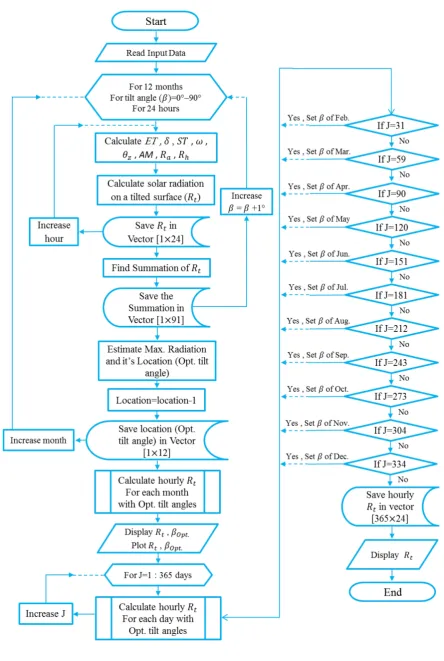
In this work, MATLAB R2014a software is used in order to estimate the optimum tilt angle and hence the hourly solar radiation on tilted surface according to optimized tilt angle for each month during the year. The proposed algorithm is as shown in the flowchart in Figure 9. The input data of the program can be classified into two types:

1. Constant input data which represent the data that doesn’t change for any case study those are: solar constant, azimuth angle, day number and local standard time as illustrated in Table 2.

Table 2. Constant input data.

Parameter Value

Solar constant (Rsc) 1.367 Azimuth angle ( ) 0° Day number (J) 1→365 Local standard time (LT) 1→24 Tilt angel ( ) 0°→90°

2. Variable input data which are representing the changed data according to the case study those are: latitude, longitude and standard meridians of local time zone, as illustrated in Table 3.

Table 3. Variable input data.

City Latitude Longitude Standard _meridian

Najaf 32.0259° 44.3462° 45°

California 36.7782° 119.4179° 120° New Delhi 28.6448° 77.2167° 82.5°

The steps of the simulated program are:

Step 1: Reading the input data which are: solar constant, azimuth angle, latitude, longitude, and standard meridian of longitude.

Step 2: Using for – loop with 12 months, LT from 1 to 24 hours, tilt angle (β) ranges from 0° to 90°.

Step 3: Calculate equation of time (ET) according to Eq. 9, declination angle (δ) according to Eq. 6, solar time (ST) according to Eq. 8, hour angle (ω) according to Eq. 7, zenith angle (θz) according to Eq. 5, air mass (AM) according to

Eq. 3, extra-terrestrial radiation (Ra) according to Eq. 4,

horizontal (Rh) radiation according to Eq. 2.

Step 4: Calculate the solar radiation on a tilted surface (Rt)

for each hour during the day using Eq.1 and Eq. 12.

Step 5: Save Rt in vector [1 × 24], and take the next hour to

calculate Rt until complete 24 hours. Then, find the

summation of the resulted Rt vector.

Step 6: Save the summation of Rt in vector of size [1 × 91].

Because of the range of tilt angle from (0° - 90°) with step of 1°, the vector size should save 90 values of tilted solar radiation and each value for an angle. The vector size is

started from 1 and ended at 91 since there is no zero size vector, therefor the results has been shifted in saving.

Step 7: Increase tilt angle (β) with step angle of 1°, and repeat the mathematical operations (step 3, 4, 5, 6).

Step 8: Estimate the maximum value of the summed tilted solar radiation in vector [1 × 91], then find its location. Location represents the optimal tilt angle at that month. It is noted that the location (optimum tilt angle) is decreased by 1, because the shifting of the saved results.

Step 9: Save the optimal tilt angle in vector [1 × 12]. Then increase the month number to repeat the previous steps for calculating the optimal tilt angle of the next month with same procedure until complete for 12 months.

Step 10 : Calculate the hourly tilted solar radiation for each month with their optimal tilt angles.

Step 11 : Display results (Rt, βoptimal) on command window

and plot them.

Step 12 : For 365 days, calculate the hourly tilted solar radiation for each day during the year with their optimal tilt angles for each month based on if – condition illustrated in Figure 9.

Step 13 : Display vector with size [365 days × 24 hours], and end the program.

4. Results and Discussion

After simulation the proposed flowchart for estimation optimal tilt angle with their solar radiation, the obtained results for each case study will be discussed as follows.

4.1. Najaf

The first case study of this work is Najaf city, where it lies in the south of Iraq. The input data of the program for Najaf city are latitude, longitude and its standard meridian and their values are 32.0259°, 44.3462° and 45° respectively. The output of the simulated program of the proposed MATLAB m-file is as follows:

1. Values of the optimal tilt angles for each month during the year of Najaf city (or other case study). This output can be seen in command window of MATLAB program. As well as of monthly optimal tilt angle, the annually optimal tilt angle is calculated.

2. Hourly average solar radiation data for each month based on their monthly optimum tilt angles. This output also appears on the command window.

3. On command window, hourly solar radiation data for 365 day of the year based on optimum tilt angle for each month can be seen.

4. The plots and waveforms of the monthly optimal tilt angles and hourly average solar insolation for each month.

.

1 2 3 4 5 6 7 8 9 10 11 12 0

10 20 30 40 50 60

Month No.

O

pt

im

al t

ilt

a

ng

le

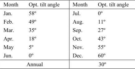
Figure 10. Monthly optimal tilt angle using MATLAB for Najaf city.

Table 4. Monthly optimal tilt angle using MATLAB for Najaf city.

Month Opt. tilt angle Month Opt. tilt angle

Jan. 58º Jul. 0º

Feb. 49º Aug. 11º

Mar. 35º Sep. 27º

Apr. 18º Oct. 43º

May 5º Nov. 55º

Jun. 0º Dec. 60º

Annual 30º

It is obvious that the wintery months (October, November, December, January, February and March) have a high values of tilt angle those are: 43°, 55°, 60°, 58°, 49° and 35° respectively. This is because the closeness of the sun to the horizon, so it is necessary to decline the solar panels. Contrariwise, the summer months (April, May, June, July, August and September) have a low values of tilt angle those are: 18°, 5°, 0°, 0°, 11° and 27° respectively, because the position of the sun is away from the horizon and closest to the verticality.

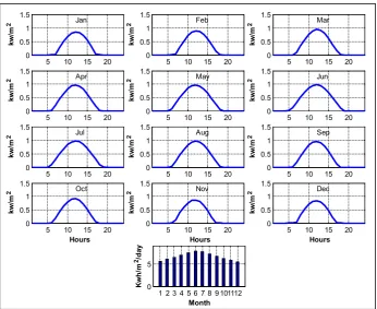
The method of changing the tilt angle each month is used in the small solar PV systems since it is easy to change the declination of solar panels. While in the large-scale PV systems, monthly changing in the tilt angle is difficult, so that, the yearly optimal declination angle is proposed as explained in the previous table. It is obvious that the annually optimum tilt angle is approached or equal to the latitude of Najaf city, and this conclusion is very well-known for whom concerned and interested researchers in the solar energy systems. The hourly solar radiation for each day during each month with monthly optimal tilt angle based on MATLAB software is as shown in Figure 11. The optimized solar radiation data in kW/m2 _{unit are illustrated} in Table 5.

For comparison purposes, the annually and monthly solar radiation on horizontal surface and tilted surface can be noted in Figure 12. and Figure 13.

It is seen from Figure 13 that the solar radiation for horizontal solar panels is less than of that for tilted surfaces. But summery months (May, June and July) have the same radiation for horizontal and tilted solar cells because the optimum tilt angle for these months are equals to zero.

It is important to study the benefits from optimization solar tilt angle in order to maximize the solar generation. The gain of watts per meter square (solar radiation energy) from tilting solar panels can be seen in Table 6.

It is obvious that the annually gain of solar radiation from tilting solar cells equals 18%, and this percentage is moderately low since the gain is zero in summer months and in winter months approximately equals 35% resulting a low gain in annually tilted solar radiation. In summer, the gain equals to zero because the solar tilt angle equals 0° in which the same angle in horizontal solar radiation. While in winter, the benefit of solar radiation from tilted surface is high and this belong to the position of the sun in the sky where it is much close to the horizon, so that, more tilting of solar panels will maximize the solar radiation energy.

4.2. California

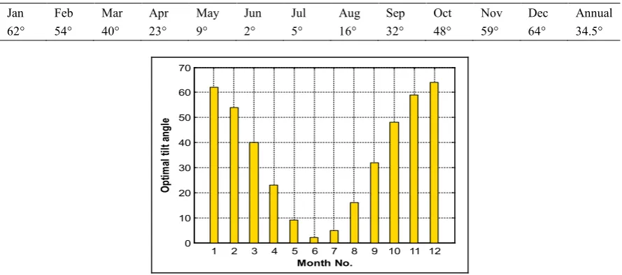
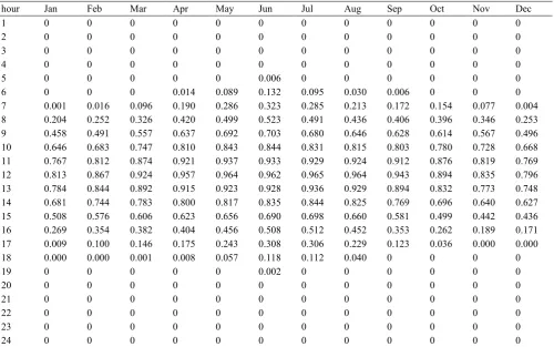
The other case study of this work is California, which has an 36.7782° latitude and 119.4179° longitude. The designed algorithm for optimization the solar tilt angle is a general program and can be applied for any case study after changing the longitude and latitude of the concerned case study. So, the obtained result after simulation the MATLAB m-file proposed software for California city can be illustrated in Table 7., in which optimized solar tilt angles for each month are shown. Also, it can be seen in Figure 14. The hourly solar radiation for each day during each month with monthly optimal tilt angle based on MATLAB software is as shown in Figure 15. The optimized solar radiation data in kW/m2 _{unit are illustrated in Table 8.}

4.3. New Delhi

The last case study of this work is New Delhi, and the optimum tilt angle can be illustrated in Table 9. and as shown in Figure 16.

5 10 15 20 0 0.5 1 1.5 kw /m 2 Jan

5 10 15 20 0 0.5 1 1.5 kw /m 2 Feb

5 10 15 20 0 0.5 1 1.5 kw /m 2 Mar

5 10 15 20 0 0.5 1 1.5 kw /m 2 Apr

5 10 15 20 0 0.5 1 1.5 kw /m 2 May

5 10 15 20 0 0.5 1 1.5 kw /m 2 Jun

5 10 15 20 0 0.5 1 1.5 kw /m 2 Jul

5 10 15 20 0 0.5 1 1.5 kw /m 2 Aug

5 10 15 20 0 0.5 1 1.5 kw /m 2 Sep

5 10 15 20 0 0.5 1 1.5 Hours kw /m 2 Oct

5 10 15 20 0 0.5 1 1.5 Hours kw /m 2 Nov

5 10 15 20 0 0.5 1 1.5 Hours kw /m 2 Dec

1 2 3 4 5 6 7 8 9101112 0 5 Month Kw h/ m 2/d ay

Figure 11. Daily hourly solar radiation for each month with optimum tilt angle using MATLAB program in Najaf city.

Table 5. Optimized solar radiation data for Najaf city in kW/m2 _unit.

hour Jan Feb Mar Apr May Jun Jul Aug Sep Oct Nov Dec Annual

1 0 0 0 0 0 0 0 0 0 0 0 0 0

2 0 0 0 0 0 0 0 0 0 0 0 0 0

3 0 0 0 0 0 0 0 0 0 0 0 0 0

4 0 0 0 0 0 0 0 0 0 0 0 0 0

5 0 0 0 0 0 0 0 0 0 0 0 0 0

6 0 0 0 0.013 0.082 0.115 0.088 0.028 0.006 0.001 0 0 0.028

7 0.005 0.033 0.103 0.192 0.282 0.313 0.281 0.213 0.176 0.171 0.120 0.027 0.160 8 0.258 0.280 0.338 0.425 0.500 0.520 0.491 0.439 0.414 0.415 0.385 0.311 0.398 9 0.502 0.517 0.571 0.644 0.696 0.706 0.682 0.651 0.638 0.634 0.602 0.543 0.616 10 0.685 0.709 0.763 0.819 0.849 0.853 0.834 0.821 0.815 0.801 0.760 0.710 0.785 11 0.803 0.838 0.890 0.930 0.944 0.945 0.933 0.931 0.924 0.897 0.850 0.808 0.891 12 0.849 0.893 0.940 0.966 0.972 0.974 0.969 0.970 0.956 0.915 0.865 0.835 0.925 13 0.820 0.870 0.908 0.924 0.929 0.939 0.939 0.936 0.906 0.852 0.804 0.787 0.884 14 0.718 0.769 0.798 0.807 0.821 0.842 0.846 0.830 0.779 0.715 0.671 0.669 0.772 15 0.548 0.601 0.619 0.628 0.657 0.691 0.699 0.663 0.590 0.516 0.476 0.483 0.598 16 0.318 0.379 0.393 0.406 0.454 0.502 0.510 0.453 0.358 0.278 0.229 0.232 0.376 17 0.037 0.126 0.153 0.174 0.237 0.294 0.301 0.227 0.125 0.046 0.003 0.001 0.144

18 0 0 0.001 0.007 0.049 0.100 0.104 0.037 0 0 0 0 0.025

19 0 0 0 0 0 0 0 0 0 0 0 0 0

20 0 0 0 0 0 0 0 0 0 0 0 0 0

21 0 0 0 0 0 0 0 0 0 0 0 0 0

22 0 0 0 0 0 0 0 0 0 0 0 0 0

23 0 0 0 0 0 0 0 0 0 0 0 0 0

Table 6. Gain of solar radiation energy from tilting solar panels.

Month Solar radiation (β=0) Opt. tilt angles Solar radiation (βopt.) % Increase

Jan 2.96 58 5.542 47%

Feb 3.92 49 6.015 35%

Mar 5.29 35 6.477 18%

Apr 6.58 18 6.936 5%

May 7.45 5 7.473 0%

Jun 7.79 0 7.795 0%

Jul 7.68 0 7.677 0%

Aug 7.07 11 7.199 2%

Sep 5.94 27 6.687 11%

Oct 4.55 43 6.241 27%

Nov 3.35 55 5.765 42%

Dec 2.73 60 5.407 49%

Yearly 5.44 30 6.601 18%

Table 7. Monthly optimal tilt angle using MATLAB for California.

Jan Feb Mar Apr May Jun Jul Aug Sep Oct Nov Dec Annual

62° 54° 40° 23° 9° 2° 5° 16° 32° 48° 59° 64° 34.5°

1 2 3 4 5 6 7 8 9 10 11 12 0

10 20 30 40 50 60 70

Month No.

O

pt

im

al t

ilt

an

gle

Figure 14. Monthly optimal tilt angle using MATLAB for California.

Figure 12. Effect of tilt angle on hourly annual solar

5 10 15 20 0 0.5 1 1.5 kw /m 2 Jan

5 10 15 20 0 0.5 1 1.5 kw /m 2 Feb

5 10 15 20 0 0.5 1 1.5 kw /m 2 Mar

5 10 15 20 0 0.5 1 1.5 kw /m 2 Apr

5 10 15 20 0 0.5 1 1.5 kw /m 2 May

5 10 15 20 0 0.5 1 1.5 kw /m 2 Jun

5 10 15 20 0 0.5 1 1.5 kw /m 2 Jul

5 10 15 20 0 0.5 1 1.5 kw /m 2 Aug

5 10 15 20 0 0.5 1 1.5 kw /m 2 Sep

5 10 15 20 0 0.5 1 1.5 Hours kw /m 2 Oct

5 10 15 20 0 0.5 1 1.5 Hours kw /m 2 Nov

5 10 15 20 0 0.5 1 1.5 Hours kw /m 2 Dec

1 2 3 4 5 6 7 8 9 101112 0 5 Month Kw h/ m 2/d ay

Figure 15. Daily hourly solar radiation for each month with optimum tilt angle using MATLAB program in California city.

Table 8. Optimized solar radiation data for California city in kW/m2 _unit.

hour Jan Feb Mar Apr May Jun Jul Aug Sep Oct Nov Dec

1 0 0 0 0 0 0 0 0 0 0 0 0

2 0 0 0 0 0 0 0 0 0 0 0 0

3 0 0 0 0 0 0 0 0 0 0 0 0

4 0 0 0 0 0 0 0 0 0 0 0 0

5 0 0 0 0 0 0.006 0 0 0 0 0 0

6 0 0 0 0.014 0.089 0.132 0.095 0.030 0.006 0 0 0

7 0.001 0.016 0.096 0.190 0.286 0.323 0.285 0.213 0.172 0.154 0.077 0.004 8 0.204 0.252 0.326 0.420 0.499 0.523 0.491 0.436 0.406 0.396 0.346 0.253 9 0.458 0.491 0.557 0.637 0.692 0.703 0.680 0.646 0.628 0.614 0.567 0.496 10 0.646 0.683 0.747 0.810 0.843 0.844 0.831 0.815 0.803 0.780 0.728 0.668 11 0.767 0.812 0.874 0.921 0.937 0.933 0.929 0.924 0.912 0.876 0.819 0.769 12 0.813 0.867 0.924 0.957 0.964 0.962 0.965 0.964 0.943 0.894 0.835 0.796 13 0.784 0.844 0.892 0.915 0.923 0.928 0.936 0.929 0.894 0.832 0.773 0.748 14 0.681 0.744 0.783 0.800 0.817 0.835 0.844 0.825 0.769 0.696 0.640 0.627 15 0.508 0.576 0.606 0.623 0.656 0.690 0.698 0.660 0.581 0.499 0.442 0.436 16 0.269 0.354 0.382 0.404 0.456 0.508 0.512 0.452 0.353 0.262 0.189 0.171 17 0.009 0.100 0.146 0.175 0.243 0.308 0.306 0.229 0.123 0.036 0.000 0.000

18 0.000 0.000 0.001 0.008 0.057 0.118 0.112 0.040 0 0 0 0

19 0 0 0 0 0 0.002 0 0 0 0 0 0

20 0 0 0 0 0 0 0 0 0 0 0 0

21 0 0 0 0 0 0 0 0 0 0 0 0

22 0 0 0 0 0 0 0 0 0 0 0 0

23 0 0 0 0 0 0 0 0 0 0 0 0

Table 9. Monthly optimal tilt angle using MATLAB for New Delhi.

Jan Feb Mar Apr May Jun Jul Aug Sep Oct Nov Dec Annual

55° 46° 32° 15° 2° 0° 0° 8° 24° 40° 51° 57° 27.5°

1 2 3 4 5 6 7 8 9 10 11 12

0 10 20 30 40 50 60 Month No. O pt im al t ilt an gle

Figure 16. Monthly optimal tilt angle using MATLAB for New Delhi.

5 10 15 20

0 0.5 1 1.5 kw /m 2 Jan

5 10 15 20

0 0.5 1 1.5 kw /m 2 Feb

5 10 15 20

0 0.5 1 1.5 kw /m 2 Mar

5 10 15 20

0 0.5 1 1.5 kw /m 2 Apr

5 10 15 20

0 0.5 1 1.5 kw /m 2 May

5 10 15 20

0 0.5 1 1.5 kw /m 2 Jun

5 10 15 20

0 0.5 1 1.5 kw /m 2 Jul

5 10 15 20

0 0.5 1 1.5 kw /m 2 Aug

5 10 15 20

0 0.5 1 1.5 kw /m 2 Sep

5 10 15 20

0 0.5 1 1.5 Hours kw /m 2 Oct

5 10 15 20

0 0.5 1 1.5 Hours kw /m 2 Nov

5 10 15 20

0 0.5 1 1.5 Hours kw /m 2 Dec

1 2 3 4 5 6 7 8 9 101112 0 5 Month Kw h/ m 2/d ay

Table 10. Optimized solar radiation data for New Delhi city in kW/m2 _unit.

Hour Jan Feb Mar Apr May Jun Jul Aug Sep Oct Nov Dec

1 0 0 0 0 0 0 0 0 0 0 0 0

2 0 0 0 0 0 0 0 0 0 0 0 0

3 0 0 0 0 0 0 0 0 0 0 0 0

4 0 0 0 0 0 0 0 0 0 0 0 0

5 0 0 0 0 0 0.008 0 0 0 0 0 0

6 0 0 0 0.052 0.133 0.156 0.127 0.071 0.040 0 0 0

7 0.091 0.120 0.177 0.263 0.347 0.366 0.336 0.280 0.251 0.257 0.230 0.150 8 0.368 0.373 0.420 0.498 0.564 0.576 0.549 0.508 0.492 0.498 0.478 0.421 9 0.589 0.598 0.645 0.708 0.751 0.758 0.736 0.711 0.705 0.704 0.677 0.627 10 0.751 0.772 0.819 0.866 0.888 0.893 0.878 0.866 0.864 0.851 0.815 0.771 11 0.846 0.879 0.924 0.955 0.964 0.969 0.961 0.956 0.950 0.924 0.882 0.847 12 0.868 0.909 0.949 0.967 0.970 0.979 0.977 0.972 0.956 0.916 0.874 0.851 13 0.817 0.862 0.892 0.901 0.906 0.922 0.926 0.915 0.882 0.830 0.790 0.782 14 0.695 0.739 0.758 0.763 0.778 0.803 0.811 0.788 0.733 0.671 0.637 0.644 15 0.509 0.553 0.561 0.566 0.598 0.633 0.643 0.604 0.526 0.457 0.426 0.443 16 0.266 0.319 0.324 0.335 0.385 0.429 0.439 0.383 0.287 0.212 0.169 0.179 17 0.007 0.067 0.090 0.108 0.167 0.215 0.224 0.158 0.065 0.009 0.000 0.000

18 0 0 0 0 0.010 0.037 0.041 0.004 0 0 0 0

19 0 0 0 0 0 0.000 0 0 0 0 0 0

20 0 0 0 0 0 0 0 0 0 0 0 0

21 0 0 0 0 0 0 0 0 0 0 0 0

22 0 0 0 0 0 0 0 0 0 0 0 0

23 0 0 0 0 0 0 0 0 0 0 0 0

24 0 0 0 0 0 0 0 0 0 0 0 0

5. Conclusion

In this study, an optimization of solar tilt angle for different sites is investigated based on MATLAB software. This work is suggested to increase the solar generation by increasing the solar insolation. The proposed algorithm is general – purposes and can be implemented for any region on the earth. However, the case studies are: Najaf, California and New Delhi. The results states that the annually optimum tilt angle is approximately equal to the location latitude in which the solar cells to be set up. Annually solar radiation gains from tilting solar cells is about 18% for Najaf city. Monthly optimal angle is also presented for each case study and the estimation of solar radiation for whole year is calculated according to their optimal angles. It is concluded that the optimum tilt angles for summer months’ ranges between 0° and 30°, and hence the benefits of solar radiation energy are fairly low. While in winter months, the gain of solar energy is high because the sun is away from the horizon and the panels is tilted with angles between 30° and 60°. This work can be a germ for future work in optimization fields in solar energy systems such as azimuth angle optimization.

References

[1] C. Julian Chen, (2011) Physics of Solar Energy. (John Wiley & Sons, Inc.).

[2] John A. Duffie, William A. Beckman, (2013) Solar Engineering of Thermal Processes, 4th _{Edition. (John} Wiley & Sons, Inc.).

[3] A.Q. Jakhrani, A. K. Othman, A. R. H. Rigit1 and S. R. Samo, (2011) A Simple Method for the Estimation of Global Solar Radiation From Sunshine Hours and Other Meteorological Parameters. 2010 IEEE International Conference on Sustainable Energy Technologies (ICSET) (IEEE).

[4] M. Benghanem, (2011) Optimization of tilt angle for solar panel: Case study for Madinah, Saudi Arabia. Applied Energy 88 (4), 1427–1433.

[5] Kadir Bakirci, (2012) General Models for Optimum Tilt Angles of Solar Panels: Turkey Case Study. Renewable and Sustainable Energy Reviews 16 (8), 6149–6159.

International Renewable and Sustainable Energy Conference (IRSEC) (IEEE).

[7] T. Khatib, A. Mohamed, M. Mahmoud and K. Sopian, (2015) Optimization of the Tilt Angle of Solar Panels for Malaysia. Energy Sources, Part A: Recovery. Utilization and Environmental Effects 37 (6), 606–613.

[8] Amit Kumar Yadav and Hasmat Malik, (2015) Optimization of Tilt Angle for Installation of Solar Photovoltaic System for Six Sites in India. 2015 International Conference on Energy Economics and Environment (ICEEE) (IEEE).

[9] Tarek O. Kaddoura, Makbul A. M. Ramli, Yusuf A. Al-Turki, (2016) On the estimation of the optimum tilt angle of PV panel in Saudi Arabia. Renewable and Sustainable Energy Reviews 65, 626–634. [10] Nabila Ihaddadene, Razika Ihaddadene and

Abdeldjabbar Charika, (2017) Best Tilt Angle of Fixed Solar Conversion Systems at M’Sila Region (Algeria). 2017 2nd International Conference on Advances on Clean Energy Research (ICACER 2017), Energy Procedia 118, 63–71.

[11] Afaneen A. Abbood, Mohammed A. Salih and Hasan N. Muslim, (2017) Management of electricity peak load for residential sector in Baghdad city by using solar generation. International Journal of Energy and Environment (IJEE) 8 (1), 63–72. [12] Yuexia Lv, Pengfei Si, Xiangyang Rong, Jinyue

Yan, Ya Feng and Xiaohong Zhu, (2018) Determination of Optimum Tilt Angle and Orientation for Solar Collectors Based on Effective Solar Heat Collection. Applied Energy 219, 11–19. [13] Miqdam Tariq Chaichan and Hussein A. Kazem,

(2018) Generating Electricity Using Photovoltaic Solar Plants in Iraq. Springer.

[14] Hasan Noaman Muslim, Afaneen Alkhazraji and Mohammed Ahmed Salih, (2017) Management of Electricity Peak Load by Using Solar PV, Assessment of Feasibility Study. LAP LAMBERT Academic Publishing.

[15] Kais J. Al-Jumaily, Munya F. Al-Zuhairi and Zahraa S. Mahdi, (2012) Estimation of clear sky hourly global solar radiation in Iraq. International Journal of Energy and Environment (IJEE) 3 (5), 659–666. [16] D. Yogi Goswami, (2015) Principles of Solar

Engineering, 3rd _{Edition. (Taylor & Francis Group} -CRC Press).

[17] Yingni Jiang, (2010) Calculation of daily global solar radiation for Guangzhou, China. 2010 International Conference on Optics, Photonics and Energy Engineering (IEEE).

[18] Roger A. Messenger and Jerry Ventre, (2005) Photovoltaic Systems Engineering, 2nd _Edition. Taylor & Francis e-Library (CRC Press).

[19] Seyed Abbas Mousavi Maleki, H. Hizam and Chandima Gomes, (2017) Estimation of Hourly, Daily and Monthly Global Solar Radiation on Inclined Surfaces: Models Re-Visited. Energies 10.

[20] S.R. Wenham, M.A. Green, M.E. Watt and R. Corkish, (2007) Applied Photovoltaics, 2nd _Edition. ARC Centre for Advanced Silicon Photovoltaics and Photonics. Earthscan.

[21] Roger Messenger and Amir Abtahi, (2017) Photovoltaic Systems Engineering, 4th _Edition. Taylor & Francis Group (CRC Press).

[22] Morteza Sarailoo, Shahrokh Akhlaghi, Mandana Rezaeiahari and Hossein Sangrody, (2017) Residential Solar Panel Performance Improvement based on Optimal Intervals and Optimal Tilt Angle. 2017 IEEE Power & Energy Society General Meeting (IEEE).

[23] N. D. Kaushika, Anuradha Mishra and Anil K. Rai, (2018) Solar Photovoltaics Technology, System Design, Reliability and Viability. Springer.

[24] A. Ben Othman, K. Belkilani and M. Besbes, (2018) Global Solar Radiation on Tilted Surfaces in Tunisia: Measurement, Estimation and Gained Energy Assessments. Energy Reports 4, 101–109. [25] Viorel Badescu, (2008) Modeling Solar Radiation at

the Earth Surface. Springer.

[26] G.N. Tiwari, Arvind Tiwari and Shyam, (2016) Handbook of Solar Energy Theory. Analysis and Applications, Springer.

[27] Parimita Mohanty, Tariq Muneer and Mohan Kolhe Editors, (2016) Solar Photovoltaic System Applications. A Guidebook for Off-Grid Electrification, Springer.

[28] Djamila Rekioua and Ernest Matagne (2012) Optimization of Photovoltaic Power Systems, Modelization, Simulation and Control. Springer. [29] Basharat Jamil, Abid T. Siddiqui and Naiem Akhtar,

(2016) Estimation of Solar Radiation and Optimum Tilt Angles for South-Facing Surfaces in Humid Subtropical Climatic Region of India. Engineering Science and Technology. an International Journal, 19 (4), 1826-1835.

[30] Isuru Vidanalage, Kaamran Raahemifar, (2016) Tilt Angle Optimization for Maximum Solar Power Generation of a Solar Power Plant with Mirrors. 2016 IEEE Electrical Power and Energy Conference (EPEC).

[31] Runsheng Tang and Tong Wu, (2004) Optimal Tilt-Angles for Solar Collectors Used in China. Applied Energy 79 (3), 239–248.