GSJ: Volume 7, Issue 12, December 2019, Online: ISSN 2320-9186
www.globalscientificjournal.com
TIME SERIES ANALYSIS OF ROAD TRAFFIC ACCIDENTS IN NIGERIA
Murtala Maitama Ahmed1 Munir Mohammad 2 Abdullahi Mohammed Rashad 3 Department of Mathematics & Statistics 1,2,3
Federal Polytechnic Kaura Namoda Zamfara State – Nigeria 1,2,3
murtalamaitama@gmail.com1 mungiat2015@gmail.com2 mohdrashad90@gmail.com 3
Abstract:
The primary objective of this paper is to introduce the class of integer-valued autoregressive (INAR) models for the time series analysis of traffic accidents. Different types of time series count data are considered: aggregated time series data where both the spatial and temporal units of observation are relatively large and disaggregated time series data where both the spatial and temporal units are relatively small (e.g., congestion charging zone and month). The performance of the INAR models is compared with the class of Box and Jenkins real-valued models (such as ARIMA models) and Poisson and Negative Binomial (NB) models. The results suggest that the performance of the ARIMA model and the INAR Poisson model is quite similar in terms of model goodness of fit for the case of aggregated time series traffic accident data. This is because the mean of the counts is high in which case the normal approximations and the ARIMA model may be satisfactory. However, the performance of INAR Poisson model is found to be much better than that of the ARIMA model for the case of the disaggregated time series traffic accident data where the counts is relatively low. The paper ends with a discussion on the limitations of INAR models to deal with the seasonality and unobserved heterogeneity.
Keywords: Traffic accidents, Time series count data, Integer-valued autoregressive, Negative binomial, Accident prediction models
INTRODUCTION
A random variable that indicates the number of times that some event has occurred is known as a count variable such as the annual number of road traffic accidents occurred on a specific geographic entity such as country, county etc. Similar to other type of empirical data, count data also have three categories: (1) cross-sectional, (2) time-series, and (3) panel. Cross-section count data are a set of observations on the values that a count variable takes for several sample units (e.g., wards, counties, boroughs, states, countries, etc.) at the same point in time. Cross-section data have only a space dimension.
Since road traffic accidents are non-negative, integer, and random event count, the distribution of such events follow a Poisson distribution. The methodology to model accident count data are well developed. For instance, cross-sectional count data are modelled using a Poisson regression model (Kulmala, 1995). Since accident count data are normally over-dispersed (i.e., variance is greater than mean), a Negative Binomial (NB) regression model which is a Poisson-gamma mixture is more appropriate to apply (Abdel-Aty and Radwan, 2000). If such cross-sectional count data contain a lot of zero observations (i.e., excess zero-count data), then a zero-inflated Poisson (or NB) model or the Hurdle count data model is more appropriate (Land at al., 1996). If cross-sectional accident count data are truncated or censored, such as the number of fatalities per fatal accident in which the count data are truncated at one as there should be at least one fatality in a fatal accident, these data are modelled using either a truncated Poisson or a truncated NB model. If cross-sectional count data are under-reported such as the occurrence of slight injury or property-damage accidents, then an under-reported Poisson model is used. If accident count data are panel data, fixed effects (FE) Poisson (or NB) model or random effects (RE) Poisson (or NB) model is used (Chin and Quddus, 2003). For clustered panel count data, the generalised estimating equations (GEE) technique is employed.
However, there is a lack of suitable econometric models within the accident modelling literature to model time series accident count data. Normally, this type of accident data is modelled using a Poisson regression model or a NB regression model that has a prevailing assumption that observations should be independent to each other. This suggests that these models are more suitable for cross-sectional count data. Modelling time series count data using these models may result inefficient estimates of the parameters as time series data are normally serially correlated. One simple solution would be to introduce a time trend variable as an explanatory variable in the model to control for serial correlation. For example, Noland et al. (2006) used a NB model with a trend variable to study the effect of the congestion charge on traffic safety. However, there is no guarantee that this will explicitly account for the effect of serial correlation, specifically for the case of a long time series count data.
Time series models for continuous data are very well developed. Real-valued time series models, such as the autoregressive integrated moving average (ARIMA) model, introduced by Box and Jenkins (1970) have been used to model time series count data in many applications over the last few decades (e.g., Zimring 1975, Sharma and Khare, 1999, Houston and Richardson, 2002, Goh, 2005). However, when modelling non-negative integer-valued count data such as traffic accidents within a geographic entity over time, Box and Jenkins models may be inappropriate. This is mainly due to the normality assumption of errors in the ARIMA model. This largely suggests that a model is required which can take into account both the non-negative discrete property and autocorrelation of time series count data.
hold the properties of the distribution of count data and are able to deal with serial correlation, and therefore offers an alternative to the real-valued time series models and general Poisson or NB models.
This paper is organised as follows. The next section describes the class of INAR models used in this study. This is followed by a description of data sources used for the analysis. A presentation and interpretation of the results are then discussed in some detail. This paper ends with conclusions and limitations of this study.
METHODOLOGY
The model for continuous autoregressive pure time series data was introduced by Box and Jenkins (1970 ) and are now very well developed. The Box and Jenkins model such as the seasonal autoregressive integrated moving average (SARIMA) model is capable of taking into account the trend and seasonality (and hence the serial correlation) normally present in time series data. An extension of this model was proposed by (Box and Tiao, 1975) which has the ability to examine the effects of various regressors and intervention variables as explanatory variables along with the usual trend and seasonal components. This model can be expressed as follows:
t t s dt s D
B
B
B
B
e
B
B
I
y
)
1
(
)
1
)(
(
)
(
)
(
)
(
0
βX
(1)in which t is the discrete time (e.g., week, month, quarter, or year), yt is the appropriate
Box-Cox transformation of Yt, say lnYt, Yt2, or Yt itself (Box and Cox, 1964), Yt is the
dependent variable for a particular time t, It is the intervention component, X is the
deterministic effects of independent variables known as control variables (X), d is the order of the non-seasonal difference, D is the order of the seasonal difference, the subscript s is the length of seasonality (for example s=12 in case of monthly time series data),
and
are the regular and seasonal autoregressive (AR) operators,
and are the regular and seasonal MA operators,
B
andB
s are the backward shift operators, ande
tis an uncorrelated random error term with zero mean and constant variance (
2).However, the model as shown in equation (1) is suitable for real-valued time series data as the error has to be normally distributed with zero mean and constant variance. Despite this assumption, this model are being used to investigate non-negative variate time series related to a number of applications including road traffic accidents (e.g., Houston and Richardson, 2002 ; Noland et al., 2006).
There are a few major problems with the application of ARIMA models to non-negative integer-valued variables such as monthly accident count data. The first problem is the definition of the model. A real-valued autoregressive process of order 1 can be expressed as follows:
Yt
Yt1 et (2)In order to obtain an integer valued Yt the following constraints have to be imposed on
yearly road traffic accidents, the distribution is usually found to be an approximate normal and hence, the use of SARIMA model may be satisfactory as the normality assumption is less questionable. However, for a count variable in which the mean of the count is close to zero such as monthly fatal road traffic accidents within a small geographic unit, the distribution is normally skewed to the right. Therefore, the assumption of normality, or of any other symmetric distribution, is unjustified.
The class of integer-valued autoregressive processes denoted by INAR have been studied by many authors (e.g., Al-Osh and Alzaid, 1987; McKenzie, E., 1988, Brännäs, Hellström, 2001, Karlis, 2006). A natural idea of such models is to replace the deterministic effect of lagged Yt’s by a stochastic one. The approach developed replaces
the scalar multiplication between
and Yt-1 by binomial thinning which is defined asfollows. If Yt1is a non-negative integer and
[0, 1] then
1 1 1 1 , 1 , 2 1 , 1 1 ... t t Y i i t Y t tt u u u u
Y
(3)where
u
i is a sequence of independently and identically distributed Bernoulli randomvariables, independent of N , and for which Pr(ui 1)1Pr(ui 0)
. It is noticeablethat conditional onYt1,
Y
t1 is a binomial random variable, the number of successes in1
t
Y independent trials in each of which the probability of success is
. Thus, the original real-valued AR(1) model of equation (2) is replaced byt t
t
Y
e
Y
1
(4)The thinning operation of
on Yt1 is independent ofe
t. The second part of equation (4)consists of the elements which entered the system during the interval
t1,t
known as innovations. The basic derivation of the INAR process is based on the assumption that the innovations,e
thas an independently and identically Poisson distribution i.e.,) (
~ t
t Poisson
e
where
tis the Poisson mean denoted by
t exp(
Xt
0It) (5)The properties of the model in equation (3) can be found in Al-Osh and Alzaid (1987) and MaKenzie (1988). The mean and variance of the process
Y
t are equal to
/(
1
)
. Equation (4) is termed as the Poisson INAR(1).Extensions of this model includes the Poisson INMA(1), the Poisson INARMA(1,1), the NB INAR(1) model, and INARMA(1,1,) NB model which has the ability to deal with both under-dispersed and over-under-dispersed count data (Al-Osh and Alzaid, 1988; Brännäs and Hall, 2001, Karlis, 2006) . Equation (3) can be estimated using the programmable Exact Maximum (EM) algorithm (Karlis, 2006).
DATA
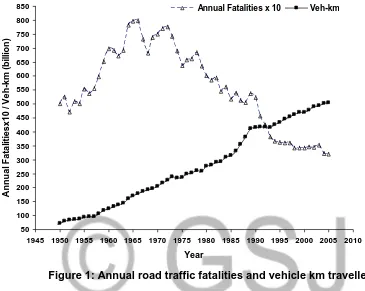
The highly aggregated time series data considered in this study is the annual road traffic fatalities in Nigeria between 1950 to 2005. The total number of observations is 55 and the mean and standard deviation of this time series process are 5,769 and 1,352 respectively. It is very well known that an accident model should contain an exposure to accident variable to control for total road traffic movements within the road network. The literature suggests that a good exposure to accident variable is vehicle kilometres travelled (VKT).
50 100 150 200 250 300 350 400 450 500 550 600 650 700 750 800 850
1945 1950 1955 1960 1965 1970 1975 1980 1985 1990 1995 2000 2005 2010
Year
A
n
n
u
a
l
F
a
ta
li
ti
e
s
x
1
0
/
V
e
h
-k
m
(
b
il
li
o
n
)
Annual Fatalities x 10 Veh-km
Figure 1: Annual road traffic fatalities and vehicle km travelled
0 2 4 6 8 10 12 14 16 18 20
May-90
Sep-91 Jan-93 Jun-94 Oct-95 Mar-97 Jul-98 Dec-99 Apr-01 Sep-02 Jan-04 May-05
Oct-06
Time (Months)
C
a
r
K
S
I
Introduction of the congestion charge charge
RESULTS
Different accident prediction models are developed using the econometric models such as ARIMA, NB, NB with a time trend, and INAR Poisson models as described in the methodology section for both aggregated and disaggregated time series datasets. Our main objective is to identify the best accident model for each type of time series datasets. For this purpose, each of the datasets is divided into two parts. One part is used to fit a model and the other part is used to validate the corresponding model. The results for each of the datasets are presented below.
Annual Road Traffic Fatalities in Nigeria (Aggregated Time Series Process)
It is worthwhile to note that the other models considered in this study such as NB, NB with a time trend, and INAR Poisson models assume that the underlying time series process is a stationary process and therefore, there is no need to manipulate the response variable of the process.
The results of ARIMA, NB, NB with a time trend variable and INAR Poisson models are presented in Table 1. In each of these models, two interventions and one control variables are used as the explanatory variables and the annual road traffic fatalities is used as a response variable. The first intervention variable is the introduction of the seat-belt law in 1983 and the second intervention variable is the introduction of various safety legislations in 1989. Both of these intervention variables are dummy variables represented by the so-called step functions. This suggests that these interventions cause an immediate and permanent effect on road traffic.
Table 1: Accident prediction models for annual road traffic fatalities.
The validation dataset that contains observations from 2001 to 2005 is used to estimate the relative forecast error, RFE, (%) of each models using the following equation:
( ˆ ) 100 5 1
i i i i y y y absRFE (5)
where,
y
iis the observed annual road traffic fatalities andy
ˆ
iis the forecasted annual road traffic fatalities using the developed model.The results are shown in the last row of Table 1. The lowest RFE (2.79%) is also found in the ARIMA (1,1,1) model suggesting that the best performance model is the ARIMA (1,1,1) model both in terms of the forecasted values associated with the out of sample observations.
In terms of the significant variables in the models, the two best performance models provide dissimilar results. Both intervention variables are found to be insignificant in the ARIMA model but found to be significant in the INAR(1) model. Both the seat-belt wearing law in 1983 and the different safety legislations in 1989 have a negative impact on road traffic fatalities in the NIGERIA in the INAR(1) model. This finding is consistent with the finding of other studies on seat-belt safety law (e.g., Houston and Richardson, 2002).
3000 3200 3400 3600 3800 4000 4200 4400 4600 4800 5000 5200 5400 5600 5800 6000
1985 1986 1987 1988 1989 1990 1991 1992 1993 1994 1995 1996 1997 1998 1999 2000 2001 2002 2003 2004 2005 2006 2007
Year O b s e rv e d / P re d ic te d f a ta li ti e s Observed
Predicted by ARIMA
Predicted by NB with a time trend Predicted by INAR Poisson
Within Sample Out of Sample
The results of SARIMA, NB, NB with a time trend, and INAR(1) Poisson models are presented in Table 2. Each of these models has an intervention variable and a control variable. The intervention variable is the introduction of the congestion charge in February 2003 which is assumed as a step function. The control variable is the total monthly road traffic accidents which is a direct measure of exposure to risk. It can be seen that the intervention variable, the introduction of the congestion charge, is statistically significant in all models except in the SARIMA model. The coefficient value of this variable is found to be -0.41 in the INAR(1) model suggesting that the introduction of the congestion charging zone within central reduces car KSI by about 33% if all other factors remain constant. The control variable is statistically significant in the INAR(1) Poisson model only. Based on the various “Measures of Accuracy” and “Relative Forecast Error” of the developed models, it can be said that the best performance model is the INAR(1) Poisson model. The RFE for the INAR(1) Poisson model is only 2.21%. The worst performance model is the SARIMA model for which the RFE is 9.03%.
Table 2: Accident prediction models for monthly car KSI within the congestion charging zone
Explanatory Variables Coeff t-stat Coeff t-stat Coeff t-stat Coeff t-stat Congestion charge -1.4505 -1.12 -0.4251 -2.25 -0.3191 -1.63 -0.4081 -2.50
ln(Monthly Accidents) 1.5802 0.32 0.8363 1.59 0.5163 0.95 0.8372 1.95
Time trend (Linear) - - - - -0.0021 -1.9 -
-Constant - -4.8670 -1.15 -2.1394 -0.48 -4.9782 -1.44
Non-seasonal MA1 0.9928 3.87 - - -
-Seasonal MA1 0.8933 7.76 - - -
-Descriptive statistics
Overdispersion parameter 0.1397 4.02 0.1326 3.9
Thinning parameter 0.0973 2.03
Series of length 168 168
Number of residuals 155 168
Accuracy of the fitted models (within sample)
Mean Absolute % error (MAPE) Mean Absolute Deviation (MAD) Mean Squared Deviation (MSD) Root Mean Sqaure Error (RMSE) Relative forecast error (%) (Out of
sample, Jan 2005 to Oct 2005) 9.03 5.12 5.31 2.21
2.48 2.33 2.36 1.53
6.15 5.45 5.56 2.33
1.75 0.96 1.01 0.64
NB with a time trend INAR(1) Poisson
22.38 16.98 17.21 7.59
Disaggregate Time Series Accident Count Data (Monthly Car KSI within the Congestion Charging Zone 1991 - 2004)
SARIMA NB
results of the disaggregated time series data while the real-valued time series model provides the worst performance among all models. The INAR(1) Poisson model provides good results for both datasets.
In terms of identifying the effects of interventions, the ARIMA model provides an unrealistic result for both time series datasets. The exact causes have not been identified. However, one of the reasons may be that the AR and MA components of this model weaken the impact of interventions.
CONCLUSIONS
Accident prediction models for time series count data were developed employing a range of econometric models such as ARIMA, NB, NB with a time trend, and INAR(1) Poisson models. Two time series accident count datasets were used to develop the accident models in this study. One of the datasets was a highly aggregated time series process of annual road traffic fatalities and the other dataset was a disaggregated time series process of monthly car KSI within the congestion charging zone. Both of the datasets had a problem of serial correlation. Each of these datasets was used to develop four accident prediction models based on the four econometric models while controlling for exposure to risk of accidents. The performance of the fitted models was investigated using various “Measures of Accuracy” for within sample observations and “Relative Forecast Error” for out of sample observations. The results implied that the best accident prediction model for the aggregated time series count data was achieved when the ARIMA model was used. The performance of INAR(1) Poisson model was also found to be good for this dataset. On the other hand, the best accident prediction model for the disaggregated time series count data was achieved when the INAR(1) Poisson model was used. This largely suggests that the controlling of both serial correlation and non-negative discrete property of count data are important when the mean of the counts is relatively high. The preserving of integer structure of the count data is more important than the controlling of serial correlation if the mean of the counts is relatively low. Since INAR(1) Poisson model is capable of controlling both properties of time series count data, one should consider to employ this model when analysing time series accident count data.
REFERENCES
Abdel-Aty, M., Radwan E., 2000, Modeling Traffic Accident Occurrence and Involvement. Accident Analysis and Prevention 32(5), 633-642.
Al-Osh, M., Alzaid, A.A., 1987, First-order integer-valued autoregressive (INAR (1)) process. Journal of Time Series Analysis 8, 261–75.
Al-Osh, M., Alzaid, A.A., 1988 Integer-valued moving average (INMA) process. Statistical Papers 29, 281–300.
Alzaid, A. A., Al-Osh, M.,1990, An integer-valued pth-order autoregressive structure (INAR(p)) process. Journal of Applied Probability 27, 314–23.
Box, G. and Jenkins, G., 1970, Time series analysis: Forecasting and control, San Francisco: Holden-Day.
Box, G.E.P., Tiao, G.C., 1975, Intervention analysis with applications to economic and environmental problems. Journal of the American Statistical Association 70, 70-74.
Brännäs, K., Hall, A., 2001, Estimation in integer-valued moving average models. Applied Stochastic Models in Business and Industry 17, 277–91.
Brännäs, K., Hellström, J., 2001, Generalized integer-valued autoregression. Econometric Reviews 20, 425–43.
Chin, H.C., Quddus, M.A., 2003, Applying the random effect negative binomial model to examine traffic accident occurrence at signalized intersections, Accident Analysis & Prevention, 35(2), 253-259.
DfT (Department for Transport), 2003, Highways Economics Note No1. 2002 - Valuation of the benefits of prevention of road accidents and casualties. Department for Transport, NIGERIA.
DfT (Department for Transport), 2006, Transport statistics Great Britain, 32nd Edition, London: TSO.
Goh, B.H., 2005, The dynamic effects of the Asian financial crisis on construction demand and tender price levels in Singapore, Building and Environment, 40: 267-276.
Houston, D.J., Richardson, L.E., 2002, Traffic safety and the switch to a primary seat belt law: the California experience, Accident Analysis and Prevention 34: 743–751.
Karlis, D., 2006, Time series model for count data, Paper presented at the Annual Conference of the Transportation Research Board, Wahsington, D.C.
Kulmala, R., 1995, Safety at Rural Three-and Four-arm Junctions: Development and Application of Accident Prediction Models. VTT publications. Espoo: Technical Research Center at Finland.
Land, K.C., McCall, P.L., Nagin, D.S., 1996, A Comparison of Poisson, Negative Binomial and Semi-parametric Mixed Poisson Regressive Models with Empirical
McKenzie, E. , 1988, Some ARMA models for dependent sequences of Poisson counts. Advances in Applied Probability 20, 822–35.
Noland, R. B., Quddus, M.A, 2004, Improvements in Medical Care and Technology and Reductions in Traffic-related Fatalities in Great Britain, Accident Analysis and Prevention, 36(1): 103-113.
Noland, R.B., Quddus, M.A. and Ochieng, W.Y., 2006, The effect of the congestion charge on traffic casualties in London: an intervention analysis, Presented at the
Transportation Research Board (TRB) Annual Meeting, Washington, D.C., USA, January.
Sharma, P., Khare, M., 1999, Application of intervention analysis for assessing the effectiveness of CO pollution control legislation in India, Transportation Research Part D 4: 427-432.