Genetic Algorithm Parameter Control: Application to Scheduling with Sequence-Dependent Setups

(1)

Genetic Algorithm Parameter Control: Application to

Scheduling with Sequence-Dependent Setups

Vincent A. Cicirello

Computer Science and Information Systems Stockton University

101 Vera King Farris Drive Galloway, NJ, 08205

[email protected]

ABSTRACT

Genetic algorithms, and other forms of evolutionary com-putation, are controlled by numerous parameters, such as crossover and mutation rates, population size, among oth-ers depending upon the specific form of evolutionary com-putation as well as which operators are employed. Setting the values for these parameters is no simple task. In this paper, we develop a genetic algorithm with adaptive con-trol parameters for an NP-Hard scheduling problem known as weighted tardiness scheduling with sequence-dependent setups. Our genetic algorithm uses the permutation repre-sentation along with the non-wrapping order crossover and insertion mutation operators. We encode the control pa-rameters within the members of the population and evolve these during search using Gaussian mutation. We demon-strate this approach out-performs a manually tuned genetic algorithm for the problem, and that it converges upon effec-tive parameter values very early in the run.

Categories and Subject Descriptors

I.2.8 [Artificial Intelligence]: Problem Solving, Control

Methods, and Search—heuristic methods, scheduling; I.2.6

[Artificial Intelligence]: Learning—parameter learning;

F.2.2 [Analysis of Algorithms and Problem

Complex-ity]: Nonnumerical Algorithms and Problems—sequencing

and scheduling, computations on discrete structures; G.2.1 [Discrete Mathematics]: Combinatorics—combinatorial algorithms, permutations and combinations

General Terms

Algorithms, Experimentation, Performance

Keywords

Genetic algorithm, parameter control, parameter optimiza-tion, permutation operators, weighted tardiness scheduling, sequence-dependent setups

1. INTRODUCTION

The Genetic Algorithm (GA) and other forms of evolu-tionary computation are typically controlled by several pa-rameters. For example, the simplest form of GA is controlled by a crossover rate, mutation rate, and population size; while more sophisticated forms have additional parameters such as elitism rate, scaling window, generation gap, or use

pa-rameterized operators such as uniform crossover ork-point

crossover. Even operator choice can be viewed as a param-eter (e.g., single-point vs two-point vs uniform crossover). The most common approach to parameter tuning is manual tuning—i.e., the GA implementer uses a tedious trial-and-error approach. Oftentimes, published results report the pa-rameter values, but do not explain how they were derived.

Others take a more rigorous approach to control param-eter tuning. De Jong offers the earliest example of formal analysis of GA control parameters, providing an empirically determined “optimal” set of parameter values for a specific class of function optimization problem [17]; while others look to automate the process, such as Grefenstette’s introduc-tion of the idea that a GA can be used to optimize GA control parameters [21]. There have since been a variety of meta-optimization approaches for optimizing GA param-eters (e.g., [25, 13, 4]), as well as the paramparam-eters of other metaheuristics (e.g., [25, 32]) and systems (e.g., [26]). Oth-ers argue that control parametOth-ers are not to be tuned a priori, but rather should adapt dynamically using feedback from search progress (e.g., [22, 18, 38, 1, 5, 15]).

In this paper, we explore an approach to dynamically adapting GA control parameters for an NP-Hard single-machine scheduling problem known as weighted tardiness scheduling with sequence-dependent setups. Our GA uses a permutation representation, rather than the classic bit-string. Many problems, such as the scheduling problem we explore here, are more naturally represented as permuta-tions of a set—in this case a set of jobs. The permutation represents the order to process the jobs. To adapt the con-trol parameters, we augment the representation to include the permutation as well as the crossover and mutation rates, allowing the GA to evolve not only the problem’s solution, but also its own parameters. In our experiments, we see po-tential to use the approach for parameter tuning, in addition to parameter control. That is, though we focus on dynamic parameter adaptation, the final evolved parameters can po-tentially be used to control future GA runs.

We begin by providing background and related work (Sec-tion 2), including on the GA permuta(Sec-tion representa(Sec-tion and

(2)

relevant operators (Section 2.1) as well as on the target prob-lem, weighted tardiness scheduling with sequence-dependent setups (Section 2.2). We present the technical details of our adaptive GA in Section 3 and discuss our experimental re-sults in Section 4. We offer concluding remarks in Section 5.

2. BACKGROUND AND RELATED WORK

2.1 GA Permutation Operators

The permutation representation requires specialized GA operators, capable of producing valid permutations from population members. Crossover must be capable of recom-bining parts of two parent permutations to produce two valid child permutations; and mutation must be capable of pro-ducing a new permutation that is a variation of another.

There are many crossover operators available that attempt to recombine different permutation properties, and are thus relevant for different problem types. For some problems, the positions of the elements within the permutation are most important, such as assignment problems where an optimal one-to-one mapping from the elements of one set to the el-ements of another is sought (e.g., largest common subgraph and other isomorphism related problems [36, 13]). For such problems, crossover must focus on retaining absolute posi-tions of elements in the parent permutaposi-tions when form-ing children. Cycle Crossover (CX) is the best available example that does just that [29]. Other relevant, though more disruptive, operators for this problem class include Partially Matched Crossover (PMX) [20] and Uniform Par-tially Matched Crossover (UPMX) [13]. For other problems, crossover must attempt to retain relative positions of ele-ments (i.e., which eleele-ments are adjacent), such as the trav-eling salesperson, and other routing and scheduling

prob-lems. Crossover operators for relative position problems

include Order Crossover (OX) [16], Non-Wrapping Order Crossover (NWOX) [7], and Uniform Order Based Crossover (UOBX) [33]. Most relevant to this paper is NWOX, as it retains edges while minimizing positional deviation rela-tive to the original parent permutations, unlike OX which keeps edges but tends to displace elements large distances from locations in parents. For scheduling with sequence-dependent setups, edges directly impact fitness; but for the weighted tardiness scheduling objective, the general position of the permutation elements also impacts duedate achieve-ment, and thus fitness. NWOX is therefore ideal for this problem. For yet other problems, crossover must retain gen-eral pairwise element precedences, and not simply edges, in order to produce children phenotypically similar to the par-ents. Precedence Preservative Crossover (PPX) [3] is de-signed to do this, while others that may work well for such problems include NWOX, UOBX, and CX. There are yet other crossover operators that introduce problem-dependent knowledge into crossover (e.g., [28, 37, 9]).

There are relatively few commonly used permutation mu-tation operators [19, 31, 35, 12]. Among these are swap, which exchanges a random pair of elements; insertion, which removes a random element and reinserts it at a random lo-cation; reversal, which reverses the order of a random sub-permutation; and scramble, which randomizes a random sub-permutation. There also exist window-limited variants of these, which constrain distance between random element selection [10]. See [11] for a comprehensive fitness landscape analysis of mutation operator behavior on permutation

land-scapes. One of the results of that study showed insertion to be the dominant choice when directed edges most directly impact fitness, and when small positional movement is im-portant. Thus, for the same reasons that we have chosen NWOX, we use insertion mutation in our GA.

2.2 Sequence-Dependent Setup Scheduling

The weighted tardiness scheduling problem with

sequence-dependent setups consists of N jobs J = {j1, j2, . . . , jN}.

Each job jk has weight wk, duedatedk, and process time

pk. For each pair of jobs, si,k is the setup time required

prior to processing job jk if it immediately follows job ji.

Setup times are asymmetric—i.e., it is not necessarily the

case thatsi,k =sk,i. s0,k is the initial setup time required

if jobjkis processed first. The weighted tardiness objective

is to sequence the set of jobsJ to minimize:

T =

N X

k=1

wkTk= N X

k=1

wkmax(ck−dk,0), (1)

whereTkandckare the tardiness and completion time of job

jk. The completion timeckis the sum of the process times

and setup times of all jobs that come beforejkplus the setup

time and process time ofjk. Letπ(k) be the position in the

sequence of jobjk, thenckis defined as follows:

ck=

X

π(x)≤π(k),π(x)=π(y)+1

(px+sy,x). (2)

Single-machine scheduling to optimize weighted tardiness is NP-Hard even if setups are independent of job

order-ing [27]. Sen and Bagchi show that sequence-dependent

setups induce a non-order-preserving property of the evalu-ation function that greatly magnifies problem difficulty [30]. The current best available exact solver for the problem, Tanaka and Araki’s Successive Sublimation Dynamic Pro-gramming, is capable of solving all of the available bench-mark instances, but requires over two weeks of memory-intensive CPU time to solve the harder instances [34]. There-fore, it is desirable to turn to alternative approaches, such as genetic algorithms as well as other metaheuristics, that are able to more efficiently find sufficiently-optimal solutions.

In our experiments, we use the standard benchmark set for

the problem, which we previously introduced [5, 6].1 _This

benchmark set has been used by many researchers for a vari-ety of search algorithms, such as dynamic programming [34], neighborhood search [24], iterated local search [39], value-biased stochastic sampling [14], genetic algorithms [7], sim-ulated annealing [8], ant colony optimization [23], etc.

3. ADAPTIVE GENETIC ALGORITHM

Instance Preprocessing.

To minimize the impact of setup times on problem solving performance, we transform each

job,jk, increasing process time by the job’s minimum setup

time, and reducing all setup times accordingly:

smink = min

0≤i≤N,i6=ksi,k, (3)

pk=pk+smink , (4)

si,k=si,k−smink ,∀i, i6=k,0≤i≤N. (5)

1_{Currently maintained at} _{http://loki.stockton.edu/}

(3)

Additionally, following Tanaka and Araki [34] as well as

oth-ers, we eliminate any jobjk, with weightwk= 0, provided

∀x∀y, x6=y, sx,k+pk+sk,y≥sx,y.

Representation.

LetPoprefer to the GA population, and let PopSizebe the size of the population. Each individual

memberiof the population is defined as a 4-tuple as follows:

Pop_i=< Pi, Ci, Mi, σi>. Piis a permutation—in the case

of the scheduling problem we consider here, it is a

permu-tation of the set of jobs. Ci and Mi are the crossover and

mutation rates, respectively, for memberiof the population;

andσiis a parameter related to mutating the crossover and

mutation rates, which we will discuss in detail below.

Fitness Calculation.

The fitness of population member

Pop_i depends explicitly only on permutation Pi, and not

on any of the GA control parameters embedded in Popi.

Let T(Pi) be the weighted tardiness (Equation 1) for

per-mutationPi; and define fitness as follows:

fitness(Pop_i) = 1−T(Pi) + max

1≤k≤PopSizeT(Pk). (6)

Our objective is to minimizeT(Pi). By defining fitness in

this way, higher fitness values correspond to better sched-ules, and the least fit individual has fitness equal to 1.

Selection.

We use elitism to select the Emost fit popula-tion members containing unique permutapopula-tions. The elite members do not undergo crossover or mutation, and are copied into the next generation as is, ensuring that the pop-ulation always contains the best solution found thus far, and also preventing convergence upon a single solution since the

population always contains at leastEunique permutations.

We use Stochastic Universal Sampling (SUS) [2] to select

the remainingPopSize−Emembers of the population for the

next generation. AllPopSizemembers of the current

popu-lation are available for selection by SUS, including the elite

members. SUS selectsPopiwith probability proportional to

fitness(Popi) just like the more common fitness

proportion-ate selection (i.e., “weighted roulette wheel”). However, SUS

is analogous to spinning a wheel withkequidistant pointers

a single time to selectk members simultaneously, whereas

fitness proportionate selection spins a 1-pointerk times to

selectkmembers. Baker showed that SUS reduces selection

bias [2]; and it is also more efficient (e.g., only 1 random number need be generated to select an entire population).

Crossover.

In each generation, the PopSize−E non-elite

members are paired randomly. For each pair,Popi,Popj,

an arbitrary member is chosen (e.g., Pop_i from this

hypo-thetical pair). With probabilityCi(the crossover rate from

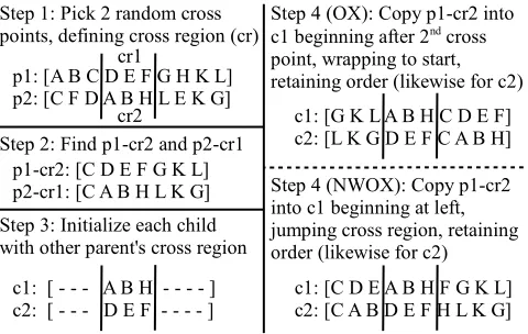
the chosen member of the pair), NWOX [7] is applied to the permutations contained in the pair. Figure 1 illustrates the behavior of both OX and NWOX for comparison. Two ran-dom cross points are chosen, similar to a 2-point bit-string

crossover. ChildCigets the cross region elements from

par-entPj in the same positions, and likewise forCj. For the

original OX [16], the remaining elements forCi are taken

in the same relative order as they appear inPi, filled into

Ci beginning just after the cross region, wrapping around

to the start. By contrast, NWOX fills in these remaining

elements beginning at the left end ofCi, skipping over the

cross region, and continuing to its end. NWOX has the

!

" ! # $ % " ! % $ #

" ! # $ % " % $ # !

& ' ( ) * * (

+ * * ,

- ./ " 0 1

+

( +

# $ % " ! % $ # ! "

- 23./ " 0

1 (

45

( +

" ! # $ % " ! % $ #

Figure 1: The NWOX and OX operators.

fect of better keeping elements near their original locations in the parents, whereas OX tends to displace elements from one end to the other of the permutation. For a scheduling problem like the one we consider here, the smaller positional displacements of NWOX is beneficial. We do not apply any crossover operation to the adaptive GA parameters.

Mutation.

In each generation, for each of thePopSize−E

non-elite members Pop_i, we apply insertion mutation with

probability Mi, the mutation rate. Insertion mutation

re-moves a random element, and then reinserts it at a different randomly chosen location, shifting the elements between the removal and reinsertion points one place each. In our prior work, we compared its performance on this very scheduling problem to alternatives both in a GA [7] as well as within simulated annealing [8]. As shown in our prior work on permutation search landscape analysis [11], insertion muta-tion is ideally suited to permutamuta-tion problems with directed edges (e.g., the asymmetric and sequence-dependent setups) and where positional information also influences fitness (e.g., general position within permutation affects job tardiness).

Parameter Initialization and Adaptation.

The initial

val-ues for the Ci and Mi are generated uniformly at random

from [0.1,1.0). These evolve during the search with

Gaus-sian mutation [22], controlled byσi. Hinterding recommends

initializing these around 0.1 [22]; and thus, we randomly

generate the initialσiuniformly from [0.05,0.15).

In each generation,Ci,Mi, andσiof each of thePopSize−

Enon-elite members undergo Gaussian mutation as follows:

Ci=Ci+N(0, σi), (7)

Mi=Mi+N(0, σi), (8)

σi=σi+N(0,0.01), (9)

where N(0, σ) is a normally distributed random variable

with mean 0 and standard deviation σ. If Ci is greater

than 1, it is reset to 1 (likewise for Mi) to ensure it

re-mains a valid probability. IfCiis less than 0.1, it is reset to

0.1 (likewise for Mi). Similarly, σi is allowed to vary only

within [0.01,0.2]. The range forσi and its adaptation rule

(4)

values of Ci and Mi are both 1; and the mid-point of the

allowable range ofσiis approximately 0.1, which is further

mutated with a Gaussian with standard deviation 0.01.

4. EXPERIMENTS

4.1 Experimental Design

The set of benchmark instances for the weighted tardiness problem with sequence-dependent setups consists of 120 in-stances, 40 each of loose duedates, medium duedates, and tight duedates. Of these, 22 instances have an optimal so-lution with weighted tardiness equal to 0 (all of these are loose duedate instances). We use the following commonly employed metrics in the analysis of our experiments for this problem. Most commonly reported is the average percentage deviation from the optimal solutions, averaged only across the instances with non-zero optimal values:

%∆Opt = 100

N N X

i=1

(Si−Oi)

Oi

, (10)

whereSiandOiare the value of the solution found for

prob-lem instancei and its optimal solution, respectively. One

problem with this metric is that it ignores the 22 problem instances whose optimal solutions have weighted tardiness equal to 0. Thus, we also report the percentage deviation of the sum across the problem instances relative to the sum of the optimal solutions:

%∆OptSum = 100 PN

i=1Si−PNi=1Oi PN

i=1Oi

. (11)

We consider the following run lengths (in maximum

num-ber of generations):{102_,₁₀3_,₁₀4_,₁₀5_,₁₀6_}_{. For each}

alter-native algorithm in our experiments, we solve each instance 10 times for each run length. The reported vales of %∆Opt

are thus averages of 10N runs (for N instances), while the

reported %∆OptSum are 10 run averages. We use t-tests to test the significance of the %∆OptSum results. How-ever, since %∆Opt is an average across multiple problem instances with values of varying scale, the normality require-ment for the t-test is not met. So we test the significance of the %∆Opt results using the Wilcoxon signed rank test.

We conduct our experiments on an Ubuntu 14.04 Server, with 32GB memory and two Intel Xeon L5520 Quad-Core CPUs (2.27GHz). The L5520 supports hyper-threading with two threads per core, so our server has a total of 16 logical cores. We implement our experiments using Java 8 and the Java HotSpot 64-bit Server VM. Our GA is not implemented with multi-threading, so it does not explicitly utilize the multi-core architecture of our server, though the VM would certainly do so for garbage collection.

We compare three GA schemes (PopSize= 100 in each):

Manually Tuned: As a baseline for comparison, we use our prior GA for the problem in which we manually tuned the GA parameters using a small set of instances not contained in the benchmark [7]. This GA also uses NWOX and In-sertion for crossover and mutation, as well as SUS selection.

The manually tuned parameters areE = 3,C = 0.95, and

M= 0.65. A mutation rate of 0.65 would be unusually high

for a bit-string GA where it is a per-bit mutation rate. How-ever, the mutation rate for a permutation-based GA is a per population member rate (i.e., the probability that a single

0.5 0.52 0.54 0.56 0.58 0.6 0.62 0.64

100 101 102 103 104 105 106

average crossover rate

generations

All instances Loose duedate instances Medium duedate instances Tight duedate instances

0.2 0.25 0.3 0.35 0.4 0.45 0.5 0.55

100 101 102 103 104 105 106

average mutation rate

generations

All instances Loose duedate instances Medium duedate instances Tight duedate instances

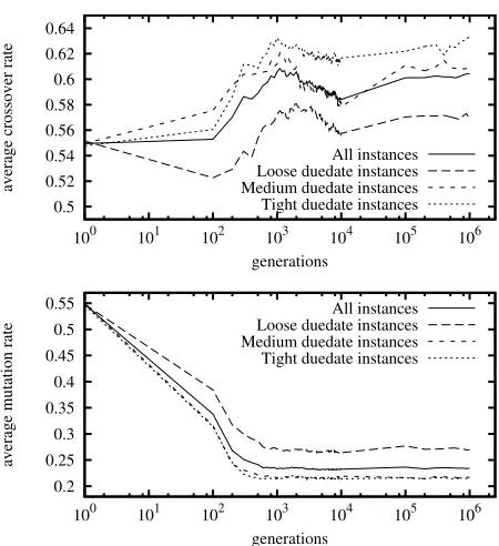
Figure 2: GA control parameter evolution: popula-tion averages across instances of designated classes.

mutation is applied to a population member), so mutation rates tend to be higher than encountered for bit-strings.

Adaptive: This is our adaptive GA as described in this

paper, where each population member has its ownCi and

Mi, which evolve during search. The elitism parameter was

tuned manually using a small set of instances outside the

benchmark, and our experiments useE= 5 retaining the 5

most fit population members unaltered in each generation. Evolved: As a third option, we consider a GA with fixed parameters derived from the final parameters of a 1000000 generation run of the GA. Figure 2 shows the evolution of the

average populationCandMaveraged across all benchmark

instances, as well as the three instance classes. For the first 10000 generations at 100 generation intervals, we computed

Cas the average of theCifor the population, andM as the

average of theMifor the population. We then continued this

at 100000 generation intervals for the remainder of the run. Note that we did not perform any cross validation and we used the very benchmark instances, so no generalizations can be made with regard to anticipated performance on future instances. This parameter set is deliberately over-fitted to serve as a performance bound with which to compare our adaptive GA—e.g., if we had access to a clairvoyant oracle that could tell us what parameters we should use, how well

would we do? The evolved parameters are: C = 0.60 and

M = 0.23 (we still useE= 5 as above).

4.2 Results

(5)

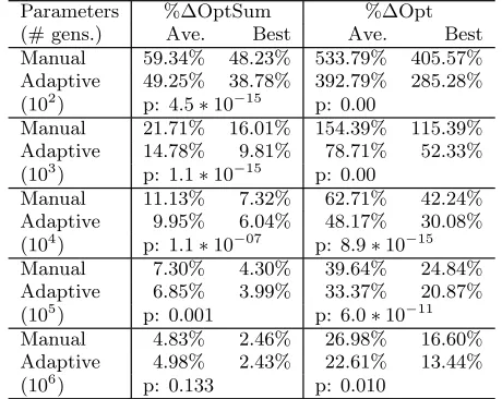
Table 1: Comparison of manually tuned parameters and adaptive parameters: %∆OptSum and%∆Opt.

Parameters %∆OptSum %∆Opt

(# gens.) Ave. Best Ave. Best

Manual 59.34% 48.23% 533.79% 405.57%

Adaptive 49.25% 38.78% 392.79% 285.28%

(102₎ _{p: 4}_.₅_∗₁₀−15 _{p: 0.00}

Manual 21.71% 16.01% 154.39% 115.39%

Adaptive 14.78% 9.81% 78.71% 52.33%

(103) p: 1.1∗10−15 _{p: 0.00}

Manual 11.13% 7.32% 62.71% 42.24%

Adaptive 9.95% 6.04% 48.17% 30.08%

(104₎ _{p: 1}_.₁_∗₁₀−07 _{p: 8}_.₉_∗₁₀−15

Manual 7.30% 4.30% 39.64% 24.84%

Adaptive 6.85% 3.99% 33.37% 20.87%

(105₎ _{p: 0.001} _{p: 6}_.₀_∗₁₀−11

Manual 4.83% 2.46% 26.98% 16.60%

Adaptive 4.98% 2.43% 22.61% 13.44%

(106) p: 0.133 p: 0.010

Table 2: Comparison of manually tuned parameters and adaptive parameters: #Opt and CPU time.

Parameters CPU

(# gens.) #Opt Time

Manual (102₎ ₃ _0.06

Adaptive (102) 7 0.05

Manual (103) 14 0.30

Adaptive (103) 121 0.19

Manual (104) 145 1.52

Adaptive (104₎ ₁₆₀ _0.87

Manual (105) 164 10.20

Adaptive (105₎ ₁₆₈ _7.15

Manual (106₎ ₁₆₉ _94.92

Adaptive (106₎ ₁₇₆ _68.51

upon a higher mutation rate and a lower crossover rate than it does for medium and tight duedates. In general, crossover rate is higher the tighter the duedates are for the instance, so crossover appears more productive than mutation for the harder, tight duedate instances.

Tables 1 and 2 summarize the experimental data compar-ing the manually tuned and the adaptive parameters. The CPU times are in seconds, averaged across 1200 runs (10 runs on each of 120 problem instances). In addition to the averages for %∆OptSum and %∆Opt, we also show the re-sults of the best runs. The #Opt is the number of runs (out of 1200) where the optimal solution was found.

Figures 3 and 4 show %∆OptSum and %∆Opt, respec-tively, averaged over all problem instances as well as by due-date tightness, as the number of generations increases. The graphs are at log-log scale.

For short runs (100 generations), the evolved fixed pa-rameters do lead to slightly better results compared to our adaptive GA across all instances of the benchmark set

(dif-ficult to see on the graphs, though p-value less than 10−10

for %∆Opt and less than 10−7 _{for %∆OptSum, shows}

dif-ferences to be extremely statistically significant for 100 gen-eration runs). However, for longer run lengths, there is no statistical significance between the performance of these two

algorithms (with the exception of loose duedate instances and runs between 10000 and 100000 generations where the fixed parameters perform slightly better). This shows that the adaptive GA needs only a small amount of time to evolve parameters that lead to effective problem solving; and that the use of sub-optimal parameters early in the run have a negligible effect on the run as a whole.

The adaptive and the evolved fixed parameters greatly out-perform the manually tuned parameters on both

met-rics with the exception of very long runs (106generations) on

tight duedate instances, where the manually tuned parame-ters lead to slightly better performance. The differences for %∆Opt between the adaptive GA and the manually tuned GA, are statistically significant for all problem classes and

all run lengths other than 105_{generation runs on tight}

due-date instances (p-value is 0.13 in that case, but is otherwise

no higher than 0.01, and in some cases less than 10−14_{). The}

%∆OptSum results are similar—i.e., statistically significant

except for 105 _{generations on tight duedate instances, and}

at 106 generations across the entire benchmark (p= 0.133).

The results are more dramatic when computational time is considered. Figure 5 shows CPU time in seconds, as a function of number of generations, averaged across all in-stances as well as separated out by duedate tightness (x-axis is at log scale). Although the adaptive GA has the added computation required to adapt the control parameters, it requires an overall lower CPU time compared to the man-ually tuned parameters. The manman-ually tuned parameters are higher crossover and mutation rates, so more GA oper-ations are performed in the same number of generoper-ations as compared to the adaptive GA. The evolved fixed parame-ters obviously require the least amount of CPU time for an equivalent number of generations. Recall that this option uses the final population average parameter values evolved by the adaptive GA, but right from the start without the added overhead of parameter adaptation.

Figure 6 shows %∆OptSum and %∆Opt, computed across the entire benchmark set, as functions of CPU time, rather than number of generations. The performance separation is more pronounced when CPU time is considered (e.g., con-trast with Figures 3a and 4a, respectively).

5. CONCLUSIONS

In this paper, we presented an adaptive GA for an NP-Hard problem: weighted tardiness scheduling with sequence-dependent setups. GA control parameters, such as mutation and crossover rates, are all too often tuned in a tedious, ad hoc trial-and-error manner. Our GA evolves the control pa-rameters simultaneously with the solution to the problem, thus eliminating the need to tune the control parameters ahead of time. An additional advantage is that the parame-ters can be tuned to the problem instance at hand dynami-cally during search. For example, we saw in Figure 2 and its associated discussion that the adaptive GA evolved a higher mutation rate and a lower crossover rate for loose duedate instances as compared to tight duedate instances.

(6)

1% 10% 100%

102 103 104 105 106

%

∆

OptSum (10 run averages)

generations

Manually tuned Adaptive Evolved

(a) All instances

10% 100% 1000% 10000%

102 103 104 105 106

%

∆

generations

(b) Loose duedate instances

10% 100% 1000%

102 103 104 105 106

%

∆

generations

(c) Medium duedate instances

1% 10% 100%

102 103 104 105 106

%

∆

generations

(d) Tight duedate instances

Figure 3: %∆OptSum (10 run averages) over: (a) all 120 benchmark instances, (b) all 40 loose duedate instances, (c) all 40 medium duedate instances, and (d) all 40 tight duedate instances.

10% 100% 1000%

102 103 104 105 106

%

∆

Opt

(980 runs = 10 runs * 98 instances)

generations

(a) All instances

10% 100% 1000% 10000%

102 103 104 105 106

%

∆

Opt

generations

10% 100% 1000%

102 103 104 105 106

%

∆

Opt

generations

1% 10% 100%

102 103 104 105 106

%

∆

Opt

generations

(7)

0 s 20 s 40 s 60 s 80 s 100 s 120 s

102 103 104 105 106

CPU time (seconds)

generations Manually tuned

Adaptive Evolved

(a) All instances

0 s 20 s 40 s 60 s 80 s 100 s 120 s

102 103 104 105 106

CPU time (seconds)

Adaptive Evolved

0 s 20 s 40 s 60 s 80 s 100 s 120 s

102 103 104 105 106

CPU time (seconds)

Adaptive Evolved

0 s 20 s 40 s 60 s 80 s 100 s 120 s

102 103 104 105 106

CPU time (seconds)

Adaptive Evolved

Figure 5: CPU time in seconds (10 run averages) over: (a) all 120 benchmark instances, (b) all 40 loose duedate instances, (c) all 40 medium duedate instances, and (d) all 40 tight duedate instances.

1% 10% 100%

0.1 s 1 s 10 s 100 s

%

∆

CPU time (seconds) Manually tuned

Adaptive Evolved

10% 100% 1000%

0.1 s 1 s 10 s 100 s

%

∆

Opt

CPU time (seconds) Manually tuned

Adaptive Evolved

Figure 6: %∆OptSum and%∆Opt expressed as func-tions of CPU time in seconds (log-log scale).

rates of crossover and mutation. We also saw that the so-lutions found by the adaptive GA are no worse than if we somehow had access to the final evolved control parameter values from the beginning. Thus, the approach efficiently converges upon effective parameter values.

We plan to further investigate the potential effectiveness of our approach for parameter tuning. For example, we saw that if we use the final average population parameter val-ues evolved by the adaptive GA right from the start of the search, that we achieve equivalent performance to the adap-tive GA but without the overhead of parameter evolution. We will investigate whether this generalizes to other yet un-seen problem instances. We will also investigate whether it is possible to bootstrap the parameter adaptation using the evolved parameters from earlier runs.

6. REFERENCES

[1] A. Aleti and I. Moser. Entropy-based adaptive range parameter control for evolutionary algorithms. In Proc. GECCO, pages 1501–1508. ACM, 2013. [2] J. E. Baker. Reducing bias and inefficiency in the

selection algorithm. InProc. ICGA, pages 14–21, 1987.

[3] C. Bierwirth, D. Mattfeld, and H. Kopfer. On permutation representations for scheduling problems. InProc. PPSN, pages 310–318. Springer, 1996. [4] J. Branke and J. A. Elomari. Meta-optimization for

parameter tuning with a flexible computing budget. In Proc. GECCO, pages 1245–1252. ACM, 2012.

[5] V. A. Cicirello.Boosting Stochastic Problem Solvers

(8)

thesis, Robotics, Carnegie Mellon University, 2003. [6] V. A. Cicirello. Weighted tardiness scheduling with

sequence-dependent setups: A benchmark library. Tech. report, ICL Lab, CMU, Feb. 2003.

http://loki.stockton.edu/~cicirelv/benchmarks/. [7] V. A. Cicirello. Non-wrapping order crossover: An

order preserving crossover operator that respects

absolute position. InProc. GECCO 2006, pages

1125–1131. ACM, July 2006.

[8] V. A. Cicirello. On the design of an adaptive simulated

annealing algorithm. InProc. CP 2007 First Workshop

on Autonomous Search. AAAI Press, Sept. 2007. [9] V. A. Cicirello. Heuristic sequencing crossover:

Integrating problem dependent heuristic knowledge

into a genetic algorithm. InProc. 23rd FLAIRS, pages

14–19. AAAI Press, 2010.

[10] V. A. Cicirello. On the effects of window-limits on the distance profiles of permutation neighborhood

operators. InProc. Int. Conf. Bioinspired Information

and Communications Technologies, pages 28–35, 2014. [11] V. A. Cicirello. The permutation in a haystack

problem and the calculus of search landscapes.IEEE

Transactions on Evolutionary Computation, Forthcoming 2016.

[12] V. A. Cicirello and R. Cernera. Profiling the distance characteristics of mutation operators for

permutation-based genetic algorithms. InProc. 26th

FLAIRS, pages 46–51. AAAI Press, May 2013. [13] V. A. Cicirello and S. F. Smith. Modeling GA

performance for control parameter optimization. In Proc. GECCO, pages 235–242, July 2000.

[14] V. A. Cicirello and S. F. Smith. Enhancing stochastic search performance by value-biased randomization of

heuristics.Journal of Heuristics, 11(1):5–34, 2005.

[15] V. A. Cicirello and S. F. Smith. The maxk-armed

bandit: A new model of exploration applied to search

heuristic selection. InProc. 20th Nat. Conf. Artificial

Intelligence, pages 1355–1361. AAAI Press, 2005. [16] L. Davis. Applying adaptive algorithms to epistatic

domains. InProc. IJCAI, pages 162–164, 1985.

[17] K. A. De Jong.An Analysis of the Behavior of a Class

of Genetic Adaptive Systems. PhD thesis, University of Michigan, Ann Arbor, MI, 1975.

[18] A. E. Eiben, R. Hinterding, and Z. Michalewicz.

Parameter control in evolutionary algorithms.IEEE

Transactions on Evolutionary Computation, 3(2):124–141, 1999.

[19] A. E. Eiben and J. E. Smith.Introduction to

Evolutionary Computing. Springer, 2003.

[20] D. E. Goldberg and R. Lingle. Alleles, loci, and the

traveling salesman problem. InProc. ICGA, pages

154–159, 1985.

[21] J. Grefenstette. Optimization of control parameters

for genetic algorithms.IEEE Transactions on

Systems, Man, and Cybernetics, 16(1):122–128, 1986. [22] R. Hinterding. Gaussian mutation and self-adaption

for numeric genetic algorithms. InIEEE CEC, pages

384–389, Nov 1995.

[23] C.-J. Liao and H.-C. Juan. An ant colony optimization for single-machine tardiness scheduling with

sequence-dependent setups.Computers and

Operations Research, 34(7):1899–1909, 2007. [24] C.-J. Liao, H.-H. Tsou, and K.-L. Huang.

Neighborhood search procedures for single machine tardiness scheduling with sequence-dependent setups. Theoretical Computer Science, 434:45–52, 2012. [25] S. Luke and A. K. A. Talukder. Is the meta-ea a

viable optimization method? InProc. GECCO, pages

1533–1540. ACM, 2013.

[26] L. D. Merkle. Metaoptimization of the in-lining priority function for a compiler targeting a

polymorphous computing architecture. InProc.

GECCO, pages 1921–1928. ACM, 2008.

[27] T. E. Morton and D. W. Pentico.Heuristic Scheduling

Systems: With Applications to Production Systems and Project Management. John Wiley and Sons, 1993. [28] Y. Nagata and S. Kobayashi. Edge assembly crossover:

A high-power genetic algorithm for the travelling

salesman problem. InProc. ICGA, pages 450–457,

1997.

[29] I. M. Oliver, D. J. Smith, and J. R. C. Holland. A study of permutation crossover operators on the

traveling salesman problem. InProc. ICGA, pages

224–230, 1987.

[30] A. K. Sen and A. Bagchi. Graph search methods for non-order-preserving evaluation functions:

Applications to job sequencing problems.Artificial

Intelligence, 86(1):43–73, 1996.

[31] M. Serpell and J. E. Smith. Self-adaptation of mutation operator and probability for permutation

representations in genetic algorithms.Evolutionary

Computation, 18(3):491–514, 2010.

[32] A. Sinha, P. Malo, P. Xu, and K. Deb. A bilevel optimization approach to automated parameter

tuning. InProc. GECCO, pages 847–854. ACM, 2014.

[33] G. Syswerda. Schedule optimization using genetic

algorithms. In L. Davis, editor,Handbook of Genetic

Algorithms. Van Nostrand Reinhold, 1991.

[34] S. Tanaka and M. Araki. An exact algorithm for the single-machine total weighted tardiness problem with

sequence-dependent setup times.Computers and

Operations Research, 40(1):344–352, 2013.

[35] C. L. Valenzuela. A study of permutation operators for minimum span frequency assignment using an

order based representation.Journal of Heuristics,

7(1):5–21, 2001.

[36] Y.-K. Wang, K.-C. Fan, and J.-T. Horng. Genetic-based search for error-correcting graph

isomorphism.IEEE Trans. Syst., Man, Cybern. B,

Cybern, 27(4):588–597, 1997.

[37] J.-P. Watson, C. Ross, V. Eisele, J. Denton, J. Bins, C. Guerra, L. D. Whitley, and A. E. Howe. The traveling salesrep problem, edge assembly crossover,

and 2-opt. InProc. PPSN, pages 823–834, 1998.

[38] S. Wessing, M. Preuss, and G. Rudolph. When parameter tuning actually is parameter control. In Proc. GECCO, pages 821–828. ACM, 2011.

[39] H. Xu, Z. L¨u, and T. C. Cheng. Iterated local search

for single-machine scheduling with sequence-dependent

setup times to minimize total weighted tardiness.J. of