Buffer management for scalable video streaming
A. Morales Figueroa
1,*, L.Favalli
11Department of Electrical, Computer and Biomedical Engineering, University of Pavia, Pavia, Italy.
Abstract
In a video streaming scenario, to cope with bandwidth variations, buffer management and intelligent drop packets policies play a critical role in the final quality of the video received at the user side. In this context, we present a buffer management strategy implemented at the source of a video communication system. This scheme uses priority information from the H.264/SVC encoder, network information from a Bandwidth Estimation approach (BE), based on Hidden Markov Model (HMM) and monitors buffer fullness: when it exceeds a defined threshold, the selective discard strategy takes place. To get more flexibility, we employed SNR quality scalability (Medium Grain Scalability), to get more than one rate point for each enhancement layer. Low priority packets correspond to higher quality layers and are discarded first, with the aim to preserve as much as possible more relevant lower layer packets. Dependencies created by the encoding process are kept into account. We show that the strategy presented ensures that the video transmitted has the highest possible quality under the given network conditions and buffer resources.
Keywords: buffer management; drop packets policy; Hidden Markov Model; bandwidth estimation; H.264/SVC; scalable video coding.
Received on 23 November 2016, accepted on 08 June 2017, published on 13 September 2017
Copyright © 2017 A. Morales Figueroa and L.Favalli, licensed to EAI. This is an open access article distributed under the terms of the Creative Commons Attribution licence (http://creativecommons.org/licenses/by/3.0/), which permits unlimited use, distribution and reproduction in any medium so long as the original work is properly cited.
doi: 10.4108/eai.13-9-2017.153337
*Corresponding author. Email:[email protected]
1. Introduction
Delivering variable bit-rate video streaming over the Internet is a challenging task. In order to guarantee the presentation quality of multimedia applications, QoS requirements such as packet loss rate, bandwidth, delay and jitter must be satisfied. Normally, transmission of video requires high bandwidth and low delay, while a certain amount of packet loss can be accepted [23].
Buffer management and scheduling algorithms represent the main class of techniques traditionally applied to maximize performance in communication networks, either wired or wireless. Video transmission makes no exception. Several works in the literature, present buffer management strategies applied to video communications that consider the specific features of video.
As an example, a study in [14] found that, for the case of low bit rate coded sequences, in most cases higher quality low
frame rate videos are preferable to lower quality full frame rate ones.
Following this consideration and the result from network analysis that outlined the fact that most of the loss occurs at the transmission point and not at the nodes inside the network, [1] proposes a simple buffer management scheme implemented at the transmission source which drops low priority packets in response to congestion, where priority is related to frame rate. In this work, the video sequences are encoded into multiple priority layers using H.26L video encoder and a robust scalable sub-band/wavelet video coder. The buffer management algorithm performs a greedy strategy on the packets being transmitted, trying to maximize the quality of the video which can be reconstructed from the transmitted packets. Basically, the algorithm constantly controls the buffer size. When the current size exceeds a defined threshold, packets are dropped considering their transmission probability. On the other hand, if the size exceeds the maximal allowed buffer size, an arriving packet is dropped without considering its priority.
In [2] the buffer management and congestion control presented in [1] are applied to video streaming. Also in this case the buffer is implemented at the source and it queues packets from the encoder and dequeued packets are transmitted using a randomized binomial scheme. The buffer algorithm is the same as the one presented in [1]. However, differently from the previous work, the Round Trip Times (RTT) are used to estimate the drop probability of a packet. An integrated video communication scheme for stored variable bit-rate (VBR) video streaming in a congested network is presented in [23]. This scheme regulates the transmission rate through a refined rate control algorithm based on the Program Clock References (PCR) value embedded in the video streams. Furthermore, multiple buffers for different importance levels, along with an intelligent selective frame discard algorithm are applied at the source. An architecture which includes an input buffer at the server coupled with the congestion control scheme of TCP at the transport layer is presented in [9]. This work assumes that the available bandwidth is sufficient to deliver the high priority frames and the goal is to maximize the number of transported low priority frames subject to the constraint that the loss rate for the high priority frames would be minimal.
In [15], different reactive and proactive queue management schemes are discussed and investigated with respect to enhancing the objective video quality of a streaming application in a HSDPA network. A proactive buffer management scheme with data differentiation is proposed, which significantly increases the video quality by taking into account MPEG frame dependencies.
Considering that a viewer can detect the discontinuity of video easier than the spatial degradation, a Weighted Multi-Playback Buffer Management (Weighted MPBuff) is proposed in [16]. The Weighted MPBuff and scheduling algorithm provides more protection to the lower layers compared to the higher ones. To archive weighted protection, the sender schedules the video data considering the transmission sequence of the video and sending different number of GOPs in each slot to build up an unequal buffer at the receiver. The playout buffer is composed by as many buffers as coded layers, and the buffer size decreases from the base layer to the highest enhancement layer. Each time period, the receiver calculates the video buffer time using the highest timestamp and the timestamp of the current playback time. This information is used to decide whether the video data unit in layer i+1 will be scheduled or not. If the current available bandwidth is not enough to transmit the layer i+1, clearly also the layers above will not be sent.
Moreover, regarding a multi-stream video transmission scenario, [6] proposes a perceptual quality-aware active queue management, which is designed for scalable video traffic. In order to reduce the queuing delay and queue length, the proposed scheme selectively drops packets from layers that have little influence on video quality, introducing a minimal perceptual quality reduction (PQR) in the stream. The dropping strategy regards the fact that losses in base quality layers cause considerably higher quality reduction than losses in quality enhancement layers. Finally, several
works have exploited scalability in wireless environments mixing with adaptive modulation and coding (AMC) and resource allocation. As an example, [12] proposes a dynamic sharing of the resources by combining SVC with appropriate radio link buffer management for multiuser streaming services. Since the pictures belonging to the lowest temporal layer are most important for decoding, these own the highest priority. Then the respective progressive refinement (PR) fragments have next lower importance, and so on. Hence, by assuming that the temporal resolution has highest priority, this work recommends a dropping order, based on the temporal level of the fragments, in case that a rate adaptation on the fly is necessary. First, the PR fragments of the present highest temporal level are dropped. If there are only packets containing base layer fragments, the base layer of the highest temporal level present is discarded. Furthermore, following the same aforementioned drop concept, this work develops a priority labeling technique, which is applied in the radio link buffer.
In this paper we present a buffer management strategy with selective packet discard for Medium Grain Scalable (MGS) video encoded H.264 video sequences, based on two main blocks:
1)A Bandwidth Estimation (BE) approach based on Hidden Markov Model (HMM), where the states sequence simulates the bandwidth of the network and are matched with the rates of the MGS encoder. 2)A selective discard of packets in the buffer based on
packet priority and its dependencies given the constraints imposed by buffer fullness and BE.
When the source transmission buffer length exceeds a given threshold, the buffer management strategy takes place, dropping low priority packets and sending the most important packets fitting the available bandwidth. Packets are discarded taking into account their quality and temporal level as defined in the MGS-SVC hierarchical dependency between layers. Base layer packets clearly have the highest priority and the packets belonging to the highest enhancement layer have the lowest one. When more than one packet has the same quality, the packet with the highest temporal level is considered to be discarded first. The algorithm developed guarantees, that the transmitted video has the highest possible quality.
The reminder of the paper is organized as follows. Section II explains the Bandwidth Estimation Model based on Hidden Markov Model and the application of this model in SVC video sequences. Section III describes the buffer management to SVC video sequences and presents the discard packets strategy proposed in this paper. Section IV presents and discusses the results obtained by the simulations. Section V gives the final conclusions and future works.
2. Bandwidth Estimation Model
relevance in several network applications. Transport layer protocols might also use AB information to change the transmission rate according to the amount of available bandwidth in the path, using the network resources efficiently while avoiding congestion [8].
Two main available bandwidth estimation approaches have been reported. The first approach is called the Probe Gap Model (PGM), which bases the estimation on the gap dispersion between two consecutive probing packets at the receiver [21]. The second approach called Probe rate model (PRM) is based on the idea of induced congestion, in which the available bandwidth is determined by the variation in the probing packet rate from sender to receiver.
This paper uses an accurate, non-intrusive and fast end-to-end approach based on PGM. Hence, using the delay variation of probe packets and the Hidden Markov Model it is possible to estimate the AB.
2.1. Hidden Markov Model
The available bandwidth can be modeled by N states, each one representing a certain level of availability. We consider a one-step transition Markov chain to estimate the probability of being in a particular state or AB range. As the available bandwidth cannot be directly observed, the probing packets approach is employed to get the delay time between packets.
Figure 1. Hidden Markov Model
Figure 1 represents the Hidden Markov Model (HMM) with discrete hidden states X representing the available bandwidth levels and discrete observation variables ξ representing probing packet pair dispersions. A particular observation has associated a probability B to be generated by a particular hidden state. Transitions between states are governed by probabilities specified in the transition probability matrix A.
As defined in [19], the Hidden Markov Model is defined by a tuple of five elements:
1. number of states (N)
2. number of distinct observation symbols per state (M) 3. state transition probability matrix (A)
4. observation probabilities (B)
5. initial state probabilities (П)
Since with MGS the video sequences are encoded with a finite number of possible rates, a finer granularity in bandwidth is not useful for our purposes. Therefore, the number of states in the model (N) is related with the number of the target bit-rates used to encode the video sequence. The set of states is defined by where the available bandwidth grows from (low) to (high). The state at time t is denoted by . The number of symbols (M) is the set of symbols denoted by
corresponding to observed dispersions from the probing sampling method. These symbols are decimal number corresponding to the delay between consecutive packets; these delay values are grouped in M intervals of values to convert every single observation to a discrete symbol.
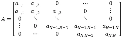
The matrix A contains the transition probability between the states. where
Since only one-step transitions between states are considered possible, the number of unknown elements in the matrix is reduced to the three main diagonals:
The matrix B has the set of probabilities that indicates how likely is that at time t a specific observation symbol is generated by each state from the set S. More specifically,
where for
and :
It is expected that the small values of ξ are the result of a highly available bandwidth and therefore more likely generated by a high index state and conversely for high values.
Given an observation sequence , that is, a set o samples from the network during T, it is desired to estimate the model that most likely generated that sequence. In order to do this, matrix A and matrix B
must be determined based on some experimental data sequence via some estimation algorithm, the most commonly used of which is the Baum Welch (BW) [18] one. Once A and B are given, the HMM can be used to generate an estimated symbol and state sequence with the same statistical properties of the original sequence.
1
X
X
t1X
tX
T1
t1
tT
... ...
A A A
The bandwidth estimation model used in this paper is based on the estimation model presented in [8]. With the purpose to analyze the implemented model and its accuracy, two experiments changing the values of the transition matrix
A and the observation probabilities B have been carried on. In the first experiment, the initial values of the A matrix are constructed using random or equally likely values. In both cases, the obtained results after the BW are quite similar. Therefore, it is possible to construct the initial matrix A (one-step transition) randomly. In the second experiment, we repeat the same procedure for the B matrix. This matrix can be constructed using random values, equally likely values or a defined pattern. This pattern considers the fact that small values of ξ (delay) are the result of a non loaded network and therefore more likely generated by a high order state (corresponding a high available bandwidth) and vice versa.
From the simulations, the last case presents higher accuracy and coherence with the expected output. The first case, random values, does not represent exactly the model but is pretty close and could be used. Furthermore, in the second case, using equally likely values, the symbol sequence constructed by the model is similar to the initial one, but the state sequence drastically varies and it is not consistent. The reason is due to the fact that matrix B does not have any specific pattern and all the states have the same occurrence probability, that it is not true.
Therefore, to generate the symbol sequence and the state sequence, in this paper, we will use a matrix A composed by random values and a matrix B made by values which represent the pattern defined in the model. Examples of the A and B matrices employed in this work are presented below, where we have 7 states (available bandwidths) and 7 symbols (delay time ranges).
Bandwidth Estimation Model applied in SVC video sequences
In SVC a signal is encoded once at the highest quality (resolution, frame rate, quality) with appropriate packetization, and then it can be decoded from partial streams for a specific rate, quality or complexity requirements [22]. There are three types of scalability: SNR scalability (fidelity), spatial scalability (resolution), and temporal scalability (frame rate). Moreover, the quality
scalability offers two options: CGS (coarse-grain quality scalable coding) and MGS (medium-grain quality scalability). In the first one, the number of available bit rates is restricted since number of layers that can be defined is not too high because it implies worse coding efficiency. MGS allows partitioning a CGS layer into several MGS layers with the aim of increasing the flexibility of bit stream adaptation and in this way improving the coding efficiency.
In this work, some test cif resolution video sequences† are encoded using the JSVM (Joint Scalable Video Model), version 9.19.15 using MGS with configuration:
, i.e. one base layer and three enhancement layers. Each of these enhancement layers defines two MGSVector. The video sequences are encoded using pre-established suitable bit-rates values obtained using the Kush Gauge [11] formula (1), based on several parameters as video width and height, frame rate and amount of motion present in the video.
. (1)
Where the motion factor could take three different values: (a) Low motion =1; (b) Medium motion =2 and (c) High motion =4.
3. Buffer management for MGS video
sequences
In a server-client adaptive streaming environment, a client makes request for multimedia objects to a centralized video server. The server sends the packets sequentially and usually selects the content from a set of files where the content is encoded at different rate to match the available bandwidth. Switching from one chunk to the other is made based on the estimates of the bandwidth obtained by some feedback mechanism based on either proprietary or standard protocols such as DASH [20]. This part is transparent to our simulation as we only assume that some information about RTT is received so that the HMM-BE model can adapt the estimated bandwidth periodically. In the present work we assume this happens every second. All encoded packets are sent to the transmission buffer. Buffer fullness obviously depends on the difference between encoding rate and available bandwidth. Losses can be reduced with larger buffers at the expenses of higher delays. We show that using scalable coded sequences and the selective discard procedure proposed, allows reducing losses while maintaining minimum delays.
When a video sequence is encoded with Scalable Video Coding, the encoded video defines one base layer and several enhancement layers, which improve the quality. In SVC, the upper layers depend upon the lower layers. In such way, if a lower layer is missing, it will not be possible to decode the above layers.
†
In this paper, we propose a Quality Discard Packets
(QDP) policy based on the above consideration regarding the priority of the packets. Hence, the base layer packets have the highest priority and the packets belonging to the highest enhancement layer have the lowest priority.
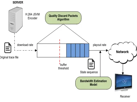
Figure 2. Quality Discard Packets scenario
The Quality Discard Packets policy is developed considering the scenario shown in Figure 2. When a H.264/SVC video is encoded, the encoder also generates a trace file which specifies various parameters for each single “packet" inside the bit-stream. The parameters include the start position (in units of bytes) of the packet, its length (in units of bytes), its values of dependency_id (Lid), its temporal level (Tid), and quality level (Qid), its type, and two flags indicating whether the packet is discardable or truncatable [10].
We set up the buffer size and define a threshold lower than the total buffer size. In this work, the threshold is equal to 50% of the maximum buffer size. When this threshold is attained, we assume the buffer is close to the risk of overflowing and the QDP policy must be applied.
The discarding packets process is governed by Algorithm 1, where is the instantaneous buffer size, MaxBufSize is
the total buffer size and BufThr is the buffer threshold indicating the buffer size at which the discard policy starts being enforced. If the queue size exceeds the threshold, the packets belonging to the highest layers, which own the highest quality, are discarded first that the other ones. Video encoded with SVC presents different temporal levels (Tid), exhibiting a hierarchical dependency. So, the packets with the highest Tid are discarded first.
On the other hand, when the queue size exceeds the imposed maximum buffer size, the arriving packet is dropped. The buffer works like a FIFO queue. At the end, the video received is decoded using the decoder tool included in JSVM
and FFMPEG [3]. Since the last one conceals whole frame losses using temporal frame interpolation, a lost P frame is concealed by copying the pixels from the previous reference frame, and a lost B frame is concealed by temporal interpolation between the frame pixels of the previous and the future frames [13].
4. Simulations results
To evaluate the performance of the Quality Discard Packets
algorithm, several cif video sequences with a duration of one minute and different characteristics, were encoded in H.264/SVC with MGS. Table 1 presents the main encoding parameters used in the Football video sequence. This video sequence which is analyzed in this section presents high spatial detail and high amount of movement.
Table 1. Encoder parameters
Football
Parameter Value
FrameRate 30
FramesToBeEncoded 1800
CgsSnrRefinement 1
MGSControl 2
GOPSize 8
BaseLayerMode 2
NumLayers 4
Original trace file download rate
buffer threshold
playout rate
Network
Receiver State sequence
Bandwidth Estimation Model Quality Discard Packets
Algorithm SERVER
The video sequences are encoded using the
FixedQPEncoderStatic tool included in the JSVM software. This tool provides two options:
Encode the video fixing the Quantization Parameter value (QP) to each layer.
Set the target bit rate that will be reached by each layer.
Here the second option is used as it allows a better match with the variations of the bandwidth conditions over the network. The following bit rates are used for a CIF sequence:
Base Layer - 200 kbps
Enhancement Layer 1 - 400 kbps
Enhancement Layer 2 - 600 kbps
Enhancement Layer 3 - 800 kbps
Moreover, each enhancement layer defines two MGSVectors, achieving in this way a video encoded with seven target points.
Using the packet size information provided by the trace file, the next step is to calculate the times when the packets arrive at the buffer from the server, as well as the times in which the packets will leave the buffer. The first one, is obtained dividing the size by the maximum bit rate at which the video was encoded. The departure time depends on the
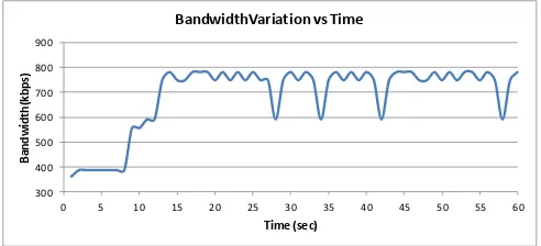
playout rate, which varies each second of time. The values of the playout rate are obtained using the Bandwidth Estimation Model presented in section II. Figure 3 shows an example of the bandwidth fluctuations, obtained with the HMM-BE model, during 60 seconds representing the duration of the employed video sequences. We selected to start with a conservative approach about bandwidth availability since it has been shown that Quality of Experience (QoE) from a user's perspective is worse when the quality is reduced along the sequence [7].
Figure 3. Bandwidth obtained with the HMM-BE model
The performance of the Quality Discard Packets
algorithm is compared with a case with No Buffer Management and a pure buffer management strategy unaware of the specific content, the Random Early Detection (RED). The RED calculates the average queue size and then, this value is compared to two thresholds: a minimum
and a maximum threshold. When the average queue
size is less than , no packets are discarded. When the
average queue is greater than , every arriving packet
is discarded. When the average queue size is between the
and thresholds, each arriving packet is
discarded with a probability , where is a function of the average queue size [5].
According to [5] , the maximum threshold should be set to at least twice the minimum one, or three times
following the rule of thumb [4]. However, a higher maximum threshold could be used in order to get a better use of buffer space and reduce the packet drops. Therefore, the RED implementation used in this work, employs a minimum and a maximum buffer threshold equivalent to the 10% and 50% of the total buffer size, respectively. Furthermore, according to [17], the RED performance is highly dependent on the thresholds and sensitive to its parameter settings. The optimization of these parameters is out of the scope of this paper.
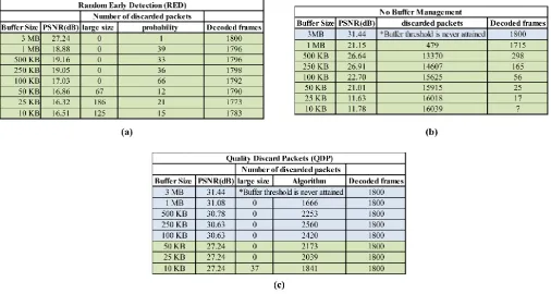
Table 2 presents the results obtained, applying the three approaches in the football video sequence. It is important to highlight that the total number of frames in the original sequence is equal to 1800 frames, corresponding to one minute of duration, and that the original trace file is composed by 16209 packets.
We can notice that in both RED and No Buffer Management cases, the buffer size must be greater or equal to 3 MB in order to get a good PSNR value recovering all the frames. However, when the QDP is used, it is possible to get a good PSNR value and recover all the frames, when a buffer size is greater or equal than 100 KB is used. This is due to the priority discard packets policy.
Considering the fact that the current version of JSVM cannot decode video streams affected by out order, corrupted or missing NALUs, we decided in these cases to use another decoder, FFMPEG, which uses error concealment techniques in order to reconstruct the original video. In Table 2, blue colored results were decoded using the JSVM decoder and the green ones were decoded with FFMPEG.
As we can see, in Table 2 (c), if FFMPEG is used for the decoding process and the QDP strategy is applied, it is possible to get an acceptable PSNR value recovering all the frames, even with a buffer size constrained. As showed in Table 2 (c), a buffer size of 10 KB presents a PSNR equal to 27.24 dB, decoding all the frames. This is possible because since we limit the number of lost packets, the concealment and recovery abilities of the FFMPEG decoder can achieve much better results.
300 400 500 600 700 800 900
0 5 10 15 20 25 30 35 40 45 50 55 60
B
and
w
idt
h(
kbp
s)
Time (sec)
Table 2. Simulations Results. (a)RED, (b) No Buffer Management and (c) QDP
In the first case, when the maximum buffer size is equal to 3MB, the QDP algorithm is not even applied because the threshold, which is established to be the 50% of the total buffer size, is not attained. The same situation occurs when any buffer management technique is used. In contrast, RED takes place when the buffer size is less or equal than 3 MB. As it is shown in Table 2 (a), one packet is discarded by the algorithm. The loss of this packet leads to that just 920 of the 1800 frames can be decoded by the JSVM decoder , and thus FFMPEG is employed.
Furthermore, we can see that even when the buffer size decreases, our Quality Discard Packets approach overcomes the other ones, recovering all the frames as the original video sequence and getting a good PSNR value. A PSNR value is considered good when it is greater than 30 dB. Moreover, when the buffer size is greater than 100 KB, the one hundred percent of the frames are recovered, attaining a PSNR equal or greater to 30.63 dB. On the other hand, to buffer sizes between 500 KB and 10 KB, all the frames are also rebuild by FFMPEG at the same time that a suitable PSNR (27.24 dB) is obtained.
It is important to mention that when a packet which is signaled as a non discardable packet in the original trace file, is discarded some distortion is inserted in the belonging frame. Moreover, as we can see in Table 2 (a), when RED algorithm is applied, the 100 percent of the decoded frames is never attained, due to its random packet discard. This
prevents further that FFMPEG reconstructs the sequence with the available packets. Consequently, the PSNR is drastically decline.
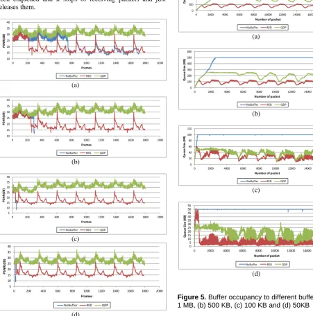
Then, Figure 4 presents the PSNR values attained by each frame of the video sequence. The PSNR of the three approaches is compared considering different buffer sizes. As can be seen in Figure 5 (a), when a buffer size of 1 MB is used, all the 1800 frames are recovered by both RED and QDP. No Buffer management reconstruct 1715 frames and this number decreases as the buffer is smaller. For instance, when the buffer size is constrained to 50KB, Figure 5 (d), only 1.4 % of the total number of frames are rebuilt.
It is worth noting that for all the cases presented in Figure 4, the QDP strategy is able to reconstruct all the frames as the original sequence and produce a good PSNR.
In order to analyze the variation of buffer occupancy, the queue size is measured each time that a packet is read from the trace file. Depending on the current queue size, the packet will be added or not to the buffer. Figure 5 illustrates the buffer occupancy, to all the three analyzed approaches, when the buffer is set to four different buffer sizes.
depending of the number of discarded packets by the QDP
strategy and the departure times of the packets. The buffer just starts decreasing when all the packets of the video have been enqueued and it stops of receiving packets and just releases them.
(a)
(b)
(c)
(d)
Figure 4. PSNR vs. Frames to different buffer sizes: (a) 1MB, (b) 500KB, (c) 100KB, (d) 50KB
As is shown in Figure 5, when No Buffer management is employed, the buffer occupancy grows until its fullness. This state is kept during all the enqueue process, then the buffer starts to be emptied. On the other hand, RED and QDP
produce a similar buffer occupancy, except that RED does not reconstruct the video sequence as the original one. Contrary to RED, which discard packets randomly, QDP
discard packets regarding its priority and influence on the other ones.
(a)
(b)
(c)
(d)
Figure 5. Buffer occupancy to different buffer sizes: (a) 1 MB, (b) 500 KB, (c) 100 KB and (d) 50KB
Moreover, we have to stress the fact that due to the "intelligent" discard packets used in our QDP approach, the buffer is never saturated, it means that any packet is dropped because the buffer is full. Hence, the possibility of losing some essential packet, which could be indispensable to the video sequence reconstruction, is reduced to zero. This does not occur with RED, where at certain time the maximum buffer size is attained (i.e. buffer sizes less or equal than 50 KB ) and the arrival packets have to be dropped.
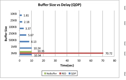
As we can see in Figure 5 (a) to (d), the buffer occupancy to the QDP is reduced significantly which corresponds to small playout delays. In Figure 6, the average delay obtained with some of the buffer sizes used to test our algorithm are showed. As aforementioned, in 3MB the QDP strategy is
10 15 20 25 30 35 40
0 200 400 600 800 1000 1200 1400 1600 1800 2000
P
SN
R(d
B)
Frames NoBuffer RED QDP
10 15 20 25 30 35 40
0 200 400 600 800 1000 1200 1400 1600 1800 2000
P
SN
R(d
B)
Frames NoBuffer RED QDP
5 10 15 20 25 30 35 40
0 200 400 600 800 1000 1200 1400 1600 1800 2000
P
SN
R(d
B)
Frames NoBuffer RED QDP
5 10 15 20 25 30 35 40
0 200 400 600 800 1000 1200 1400 1600 1800 2000
P
SN
R(d
B)
Frames
NoBuffer RED QDP
0 200 400 600 800 1000 1200
0 2000 4000 6000 8000 10000 12000 14000 16000 18000 20000
Q u eu e Si ze (K B)
Number of packet NoBuffer RED QDP
0 100 200 300 400 500 600
0 2000 4000 6000 8000 10000 12000 14000 16000 18000
Q u eu e Si ze (K B)
Number of packet NoBuffer RED QDP
0 20 40 60 80 100 120
0 2000 4000 6000 8000 10000 12000 14000 16000 18000
Q u eu e Si ze (K B)
Number of packet NoBuffer RED QDP
0 5 10 15 20 25 30 35 40 45 50 55
0 2000 4000 6000 8000 10000 12000 14000 16000 18000
Q ue ue S ize (K B )
not even applied, but when our approach takes place the delay is reduced considerably. We only compare the delay time obtained by the three approaches when the buffer size is equal to 3 MB because, just in this case all the approaches are able to recover all the 1800 frames. Moreover, blending FFMPEG and the QDP strategy as in the cases of a buffer size equal to 25 KB and 10 KB (Figure 6), the average delay is decreased to 2.18 and 1.81 seconds respectively.
It is evident that the discard packets algorithm proposed in this paper produces better results and due to its priority discard packets is possible to reconstruct the original video sequence in the highest quality available.
Work is in progress to move the analysis to a scenario where we statistically multiplex several streams and the bandwidth fluctuations affect the multiplexed stream. Furthermore, for the Bandwidth Estimation model, in this work, the initial state probabilities are set up in default mode. In such way, the initial state is the lowest state index which is related to the lowest bandwidth. This initial values could be modified in order to analyze other scenarios and buffer behavior under different networks.
Figure 6. Buffer Size vs. Delay
A final consideration is related to the applicability of the proposed approach to a large set of independent connections thus comparing it to some adaptive streaming algorithms. It is worth noting that the exploitation of scalable coding avoids the need to pre-encode a large set of copies of the same content. Furthermore, as seen from the results above, the requirements on buffer size to compensate for the bandwidth fluctuations are clearly smaller than for the other two approaches therefore reducing the latency of the transmission chain.
5. Conclusions
In this paper, we presented a discard packets strategy which considers the priority of the packets before discard them. This priority is assigned considering the quality (Qid)
and temporal (Tid) level of a packet. The proposed discard algorithm takes into account the current available network bandwidth, given by a Bandwidth Estimation Model, to apply an intelligent discard of the packets stored in the buffer. The packets are dropped from low to high priority. In the simulations, we compare our discard strategy with two other approaches and the simulations results have shown that the proposed algorithm outperforms the other two approaches and shows significant reduction in required buffer size and therefore delay. Work still needs to be performed to correctly determine the thresholds, based on the delay constraints and the type of sequence.
6. References
[1] Bajic, I.V. et al. 2003. Integrated end-to-end buffer management and congestion control for scalable video communications.
Image Processing, 2003. ICIP 2003. Proceedings. 2003
International Conference on (2003), III–257–60 vol.2.
[2] Balan, A. et al. Integrated Buffer Management and Congestion Control for Video Streaming.
[3] FFMPEG official website : http://ffmpeg.org/.
[4] Floyd, S. RED: Discussions of Setting Parameters. http://www.icir.org/floyd/REDparameters.txt
[5] Floyd, S. and Jacobson, V. 1993. Random early detection gateways for congestion avoidance. Networking, IEEE/ACM
Transactions on. 1, 4 (Aug. 1993), 397–413.
[6] Ghoreishi, S.E. et al. 2015. Perceptual quality-aware active queue management for video transmission. Personal, Indoor, and Mobile Radio Communications (PIMRC), 2015 IEEE 26th
Annual International Symposium on (Aug. 2015), 1267–1271.
[7] Grafl, M. and Timmerer, C. 2013. Representation switch smoothing for adaptive HTTP streaming. (2013), 178–183. [8] Guerrero, C.D. and Labrador, M.A. 2008. A Hidden Markov
Model approach to available bandwidth estimation and monitoring. Internet Network Management Workshop, 2008.
INM 2008. IEEE (Oct. 2008), 1–6.
[9] Gürses, E. et al. 2003. Selective frame discarding for video streaming in TCP/IP networks. Packet Video Workshop, Nantes,
France (April 2003) (2003).
[10] JSVM Software Manual, version 9. 19. 14. 2011. (2011). [11] Kush Gauge equation is available in:
https://www.adobe.com/content/dam/Adobe/en/devnet/video/art icles/h264_primer/h264_primer.pdf.
[12] Liebl, G. et al. 2006. Advancedwireless Multiuser Video Streaming using the Scalable Video Coding Extensions of H.264/MPEG4-AVC. 2006 IEEE International Conference on
Multimedia and Expo (Jul. 2006), 625–628.
[13] Lin, T.-L. et al. 2010. Subjective experiment and modeling of whole frame packet loss visibility for H.264. Packet Video
Workshop (PV), 2010 18th International (Dec. 2010), 186–192.
[14] Masry, M. and Hemami, S.S. 2001. An analysis of subjective quality in low bit rate video. Image Processing, 2001.
Proceedings. 2001 International Conference on (2001), 465–
468 vol.1.
[15] Orlov, Z. and Necker, M.C. 2007. Enhancement of video streaming QoS with active buffer management in wireless environments. European Wireless Conference (2007).
[16] Palawan, A. et al. 2014. Weighted multi-playback buffer management for scalable video streaming. Computer Science and Electronic Engineering Conference (CEEC), 2014 6th
(2014), 47–51.
10.34 10.24 8.13 5.67 3.37 2.18 1.81
70.72 10.35
0 10 20 30 40 50 60 70 80
3MB 1MB 500KB 250KB 100KB 25KB 10KB
Time(sec)
Bu
ff
er
S
iz
e
Buffer Size vs Delay (QDP)
[17] Patel, C.M. 2013. URED: Upper threshold RED an efficient congestion control algorithm. Computing, Communications and Networking Technologies (ICCCNT),2013 Fourth International
Conference on (Jul. 2013), 1–5.
[18] Poritz, A.B. 1988. Hidden Markov models: a guided tour.
Acoustics, Speech, and Signal Processing, 1988. ICASSP-88.,
1988 International Conference on (Apr. 1988), 7–13 vol.1.
[19] Rabiner, L. 1989. A tutorial on hidden Markov models and selected applications in speech recognition. Proceedings of the IEEE. 77, 2 (Feb. 1989), 257–286.
[20] Sodagar, I. 2011. The MPEG-DASH Standard for Multimedia Streaming Over the Internet. IEEE MultiMedia. 18, 4 (Apr. 2011), 62–67.
[21] Xu, D. and Qian, D. 2008. A bandwidth adaptive method for estimating end-to-end available bandwidth. Communication Systems, 2008. ICCS 2008. 11th IEEE Singapore International
Conference on (Nov. 2008), 543–548.
[22] Yang, S.-H. and Tang, W.-L. 2011. What are good CGS/MGS configurations for H.264 quality scalable coding? Signal
Processing and Multimedia Applications (SIGMAP), 2011
Proceedings of the International Conference on (Jul. 2011), 1–
6.
[23] Zhang, Y. et al. 2007. Integrated Rate Control and Buffer Management for Scalable Video Streaming. Multimedia and
Expo, 2007 IEEE International Conference on (Jul. 2007), 248–