Safe Planning And Control Of Autonomous Systems: Robust Predictive Algorithms

(1)

University of Pennsylvania University of Pennsylvania

ScholarlyCommons

Publicly Accessible Penn Dissertations

2019

Safe Planning And Control Of Autonomous Systems: Robust

Predictive Algorithms

Yash Vardhan Pant

University of Pennsylvania, [email protected]

Follow this and additional works at: https://repository.upenn.edu/edissertations

Part of the Electrical and Electronics Commons

Recommended Citation Recommended Citation

Pant, Yash Vardhan, "Safe Planning And Control Of Autonomous Systems: Robust Predictive Algorithms" (2019). Publicly Accessible Penn Dissertations. 3419.

https://repository.upenn.edu/edissertations/3419

(2)

Safe Planning And Control Of Autonomous Systems: Robust Predictive

Algorithms

Abstract Abstract

Safe autonomous operation of dynamical systems has become one of the most important

research problems. Algorithms for planning and control of such systems are now

nding place on production vehicles, and are fast becoming ubiquitous on the roads

and air-spaces. However most algorithms for such operations, that provide guarantees,

either do not scale well or rely on over-simplifying abstractions that make them

impractical for real world implementations. On the other hand, the algorithms that

are computationally tractable and amenable to implementation generally lack any

guarantees on their behavior.

In this work, we aim to bridge the gap between provable and scalable planning

and control for dynamical systems. The research covered herein can be broadly

categorized into: i) multi-agent planning with temporal logic specications, and ii)

robust predictive control that takes into account the performance of the perception

algorithms used to process information for control.

In the rst part, we focus on multi-robot systems with complicated mission requirements,

and develop a planning algorithm that can take into account a) spatial,

b) temporal and c) reactive mission requirements across multiple robots. The algorithm

not only guarantees continuous time satisfaction of the mission requirements,

but also that the generated trajectories can be followed by the robot.

The other part develops a robust, predictive control algorithm to control the

the dynamical system to follow the trajectories generated by the rst part, within

some desired bounds. This relies on a contract-based framework wherein the control

algorithm controls the dynamical system as well as a resource/quality trade-o in a

perception-based state estimation algorithm. We show that this predictive algorithm

remains feasible with respect to constraints while following a desired trajectory, and

also stabilizes the dynamical system under control.

(3)

that the planning method is computationally ecient as well as scales better than

other state-of-the art algorithms that use similar formal specications. We also show

that the robust control algorithm provides better control performance, and is also

computationally more ecient than similar algorithms that do not leverage the resource/

quality trade-o of the perception-based state estimator

Degree Type Degree Type

Dissertation

Degree Name Degree Name

Doctor of Philosophy (PhD)

Graduate Group Graduate Group

Electrical & Systems Engineering

First Advisor First Advisor

Rahul Mangharam

Subject Categories Subject Categories

(4)

SAFE PLANNING AND CONTROL OF AUTONOMOUS SYSTEMS: ROBUST PREDICTIVE ALGORITHMS

Yash Vardhan Pant

A DISSERTATION

in

Electrical and Systems Engineering

Presented to the Faculties of the University of Pennsylvania in Partial Fulfillment of the Requirements for the

Degree of Doctor of Philosophy

2019

Rahul Mangharam, Associate Professor of Electrical and Systems Engineering Supervisor of Dissertation

Victor Preciado, Associate Professor of Electrical and Systems Engineering Graduate Group Chairperson

Dissertation Committee:

George Pappas, Professor of Electrical and Systems Engineering Manfred Morari, Professor of Electrical and Systems Engineering

Georgios Fainekos, Associate Professor of Computing, Informatics and Decision Sys-tems Engineering,

Arizona State University

(5)

COPYRIGHT

2019

(6)

(7)

Acknowledgments

(8)

ABSTRACT

Yash Vardhan Pant Rahul Mangharam

Safe autonomous operation of dynamical systems has become one of the most impor-tant research problems. Algorithms for planning and control of such systems are now finding place on production vehicles, and are fast becoming ubiquitous on the roads and air-spaces. However most algorithms for such operations, that provide guaran-tees, either do not scale well or rely on over-simplifying abstractions that make them impractical for real world implementations. On the other hand, the algorithms that are computationally tractable and amenable to implementation generally lack any guarantees on their behavior.

In this work, we aim to bridge the gap between provable and scalable planning and control for dynamical systems. The research covered herein can be broadly categorized into: i) multi-agent planning with temporal logic specifications, and ii) robust predictive control that takes into account the performance of the perception algorithms used to process information for control.

In the first part, we focus on multi-robot systems with complicated mission re-quirements, and develop a planning algorithm that can take into account a) spatial, b) temporal and c) reactive mission requirements across multiple robots. The algo-rithm not only guarantees continuous time satisfaction of the mission requirements, but also that the generated trajectories can be followed by the robot.

The other part develops a robust, predictive control algorithm to control the the dynamical system to follow the trajectories generated by the first part, within some desired bounds. This relies on a contract-based framework wherein the control algorithm controls the dynamical system as well as a resource/quality trade-off in a perception-based state estimation algorithm. We show that this predictive algorithm remains feasible with respect to constraints while following a desired trajectory, and also stabilizes the dynamical system under control.

(9)

List of Tables

3.1 Example 4. Runtimes (mean and standard deviation, in seconds) for Smooth Operator (SOP) and BluSTL (BlS) in modes (B) and (R), over 100 runs with random initial states and different formula horizons N. BluSTL(R) did not finish (see text). . . 22 3.2 HVAC. Runtimes (mean ± std deviation, in seconds) SOP and BluSTL

(BlS) over 100 runs with random initial states. . . 25 3.3 Robustness of final trajectory,ρ∗, for 3 runs with different initial trajectories

(x0), none of which satisfyϕ. . . 28

4.1 Stop-and-Go motion. Mean±standard deviation for run-times (in seconds) and robustness values from 100 runs of the reach-avoid problem. . . 46 4.2 Free Endpoint Velocity motion. Mean ± standard deviation for runtimes

(in seconds) and robustness values from 100 runs of the reach-avoid problem. 47 4.3 Mean ± standard deviation for runtimes (in seconds) and robustness

val-ues for one-shot optimization. Obtained from 50 runs of the multi-mission problem with random initial positions. . . 48 4.4 Average runtime per time-step (in seconds) of shrinking horizon robustness

maximization in Boolean mode. These are averaged over 5 repetitions of the experiment from the same initial point, to demonstrate the reproducibility of the experiments. . . 52 4.5 Links for the videos for simulations and experiments. Here, Sim. stands for

Matlab simulations, CF2.0 for experiments on the Crazyflies. Stop-go and vel. free are the two modes of operation of the trajectory generator, and B (R) is the Boolean (Robust) mode of solving the control problem. Shr. Hrz. stands for the shrinking horizon mode for online control. The reader is advised to make sure while copying the link that special characters are not ignored when pasted in the browser. . . 53

(14)

List of Figures

1.1 Multiple autonomous drone missions in an urban environment. . . 1 1.2 Organization of the research contributions of this work. Chapters 3

and 4 address the problem of planning and control with temporal logic objectives, while chapters 6 and 7 address the robust predictive control problem. . . 5 1.3 Generated trajectories and robustness boxes within which to track.

The STL specification corresponds to the two drones reaching the green goal set within time interval of 6 seconds, while making sure the two drones do not enter the unsafe red set, or crash into each other. If the drones are following their trajectories within the given (blue for drone 1 and black for drone 2) boxes at the corresponding time step, then they satisfy the STL specification. Chap. 4 presents the planning method that generates these trajectories as well as the bounds within which to track them. Chap. 6 presents a control method to follow these trajectories within the given robustness boxes while taking into account the errors and delays associated with the perception-based state estimation commonly used in feedback control. . . 7

2.1 This illustration shows a UAS and two trajectories,x1 (in black) and x2 (in blue). Color in digital version. . . 11

3.1 Iterates of SQP for Example 3. Colors in online version.. . . 20 3.2 Robustness approximation error against formula horizon, evaluated on 1000

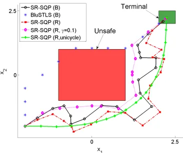
randomly generated trajectories for Example 4. Unless noted, the systems are 2D. Color in online version. . . 21 3.3 The first 4 trajectories are for Example 4. The last trajectory, SOP(R,

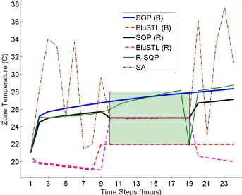
unicycle), is from Example 5. Colors in online version. . . 23 3.4 Zone temperatures. The green rectangle shows the comfortable temperature

(15)

3.5 Trajectories obtained via SQP on smooth robustness, with three different initial trajectories acting as initial solutions for the SQP. Note, all 3 tra-jectories satisfy ϕ. Here, pj_i refers to the positions of the ith _trajectory for the jth _{quadrotor. A real-time playback of trajectories can be seen in}

https://youtu.be/FU3Rg1Jb7Fw. . . 29

4.1 (Top) Five Crazyflie 2.0 quadrotors executing a reach-avoid mission. (Bot-tom) A screenshot of a simulation with 16 quadrotors. In both cases, the quadrotors have to satisfy a mission given in STL. . . 32 4.2 The control architecture. Given a mission specification in STL, the

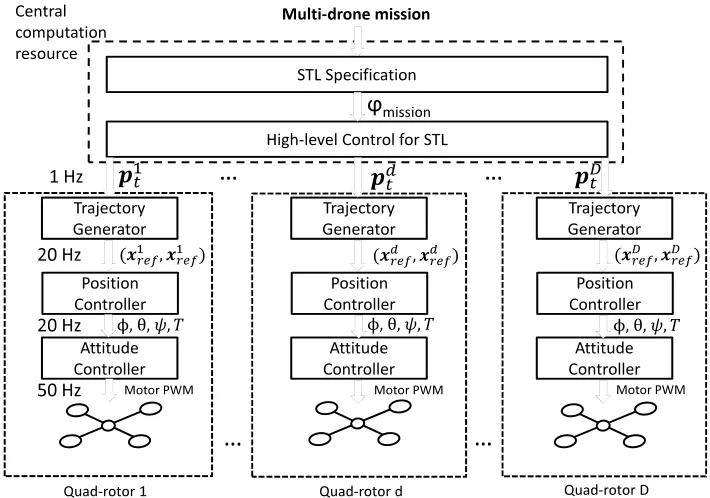
high-level control optimization (centralized) generates a sequence of waypoints. These waypoints are sent over to the drones, and through a hierarchical control on-board control architecture, the resulting trajectories are tracked near perfectly, with the continuous time behavior of the system satisfying the STL specification. . . 35 4.3 World frame and rotation angles (left) and quadrotor frame with angular

rates (right). gis gravitational force. Figure adapted from Fig. 2 in Mueller et al. [2015]. . . 36 4.4 Planar splines connecting position waypoints p0, p1 and p2. q0 is the

con-tinuous spline (positions, velocities and accelerations) connectingp0 and p1

andq1 is the spline fromp1 top2. q(kdt

0

) is thekth _{sample of}_q0_{, with}

sam-pled time dt0. Note, unlike the stop-go case, non-zero end point velocities mean that the resulting motion is not simply a line connecting the way points. 38 4.5 The upper and lower bounds on pf due to the acceleration and velocity

constraints. Shown as a function of v0 for t = 0,0.1, . . . , Tf = 1. The shaded region shows the feasible values ofpf as a function ofv0. . . 40

4.6 The functionsK1 toK4 forTf = 1. . . 42

4.7 The environment for the multi-mission problem. . . 49 4.8 The desired and actual trajectories for a Crazyflie 2.0 flying the reach-avoid

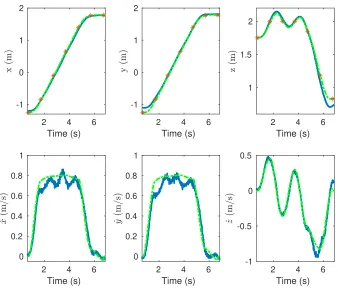
problem with closed-loop control. The unsafe set is in red and the goal set is in green (Color in online version). . . 50 4.9 The desired (dashed green) and actual (blue) positions and velocities along

(16)

5.1 The Fly-by-Logic tool-chain. Through a MATLAB-based graphical interface (fig-ure 5.2), the user defines the workspace and the multi UAS mission. This mission is interpreted as an STL specification (of the form in equation 5.1), the parameters of which are passed from the interface to the Fly-by-Logic C++ library. Through interfacing with off-the-shelf optimization tools, trajectories that satisfy the mis-sion are generated for each UAS and visualized through the user interface. The way-points that generate these trajectories can also be sent to a Robot Operating Systems (ROS) implementation of trajectory following control to be deployed on

board actual robots (e.g. bit.ly/varvel8). . . 55

5.2 The user interface and the planned trajectories for a two UAS patrolling mission (see example 6). Real-time playback can be seen at http://bit. ly/fblguiexmpl . . . 57 5.3 Trajectories for 3 UAS tasked with reaching the green-colored goal set

within 2 minutes, while avoiding the all black-colored obstacles. A pairwise separation requirement of ≥2 meters is enforced for all UAS. 60 5.4 Workspace for the PHL airport example. A 10x speedup of the planned

trajectories are shown in https://youtu.be/vBYRFfnLwu8. . . 62

6.1 Contract-driven controller and estimator. The co-design allows the controller to set acontract for the perception-based state estimator, in addition to controlling the dynamical system. . . 66 6.2 Effect of delay, error values on control performance of a PID tracker. 67 6.3 Autonomous hexrotor with downward-facing camera flying over

syn-thetic features. . . 69 6.4 Contract-driven estimator and controller. With knowledge of the

esti-mator’s performance through offline profiling, the controller both ac-tuates the dynamical system and sets contracts for the estimator at run-time in order to maximize control performance while guaranteeing that constraints on the system are always satisfied. . . 70 6.5 Time-triggered sensing and actuation. The figure shows the varying

execution time for the estimator and the blue area shows the execution time for the controller, which is small. . . 72 6.6 Illustration of the building blocks used to compose the Contract Object

Detector and their representation as real-time tasks. For a given (δ, ) contract, knob settings are chosen at run-time resulting in a schedule to execute these sequential components, or tasks, to respect the contract. 79 6.7 Profiled delay-error curve for the object detection tool chain run at

(17)

6.8 The profiling process to characterize the performance of SVO in terms of estimation error, computation time and power consumption. Sen-sor and ground truth data is logged from flights of the hexrotor, and then played back and processed offline to generate the error-delay curve (shown in Fig. 6.9) for SVO. The code snippet shows how little modi-fication is needed to the SVO code base to be able to profile its timing characteristics. Through this offline profiling process, we avoid the need of performing separate flights for each knob setting of SVO. . . . 82 6.9 (Color online) Error-delay curve for the SVO algorithm running on

the Odroid-U3 with different settings of maximum number of features (#C) to detect and track. The vertical line shows the cut-off for max-imum delay and the SVO settings that are allowable (upto #C= 200) for closed loop control of a hexrotor at 20Hz. No value of #C is used above this as it results in the delay approaching the sampling period of the controller. . . 84 6.10 The control and computational components on-board the hex-rotor. 85 6.11 The two reference trajectories, the spiral is in dashed red and the

hourglass is in solid black (color in online version). The figure on the right shows the trajectories projected on the x,y plane. Note, the spiral starts on the outside and ends inwards while the hourglass trajectory starts and ends at (0,0,1). . . 87 6.12 Performance, hourglass trajectory. The vertical axis has the

aver-age control performance (eq. 6.8) over the flights for the labeled settings,with lower values implying better control performance. The horizontal axis shows the computation power (in Joules) consumed by SVO to perform the state estimation task. The figure shows how our methods (RAMPC/SAMPC) leveraging the co-design have both bet-ter control performance while consuming less computation power than the baseline method. . . 88 6.13 Performance, spiral trajectory. The vertical axis has the average

con-trol performance (eq. (6.8)) over the flights for the labeled settings,with lower values implying better control performance. The horizontal axis shows the computation power (in Joules) consumed by SVO to per-form the state estimation task. Similar to the case for the hourglass trajectory, our methods outperform the baseline. . . 89 6.14 (Color online) Reference positions (dashed red) and actual positions

(blue) of the hex-rotor flying the hourglass trajectory while being con-trolled by the SAMPC (α = 0). . . 90 6.15 (Color online) Reference positions (dashed red) and actual positions

(18)

6.16 SVO Mode and control cost over time for the spiral trajectory flown with SAMPC at α= 0.001. . . 93 6.17 Cumulative distribution of profiled execution times for visual odometry

running on the Odroid-U3 for varying maximum number of corners from the SVO algorithm. . . 104

7.1 The outer-approximated reach sets for xk+j, computed at time steps k, k+ 1, used to compute Ee_k₊_j|k, Vk+j|k. . . 113

7.2 Local and global inner approximations of input constraints for running example, with Xk+j|k = [−π/4,0]×[−0.9666,−0.6283] for some k, j

and U = [−2.75,2.75]. Color in online version. . . 114 7.3 The error sets ˜Emax and ˜E computed over an arbitrary Xk+j|k. Also

shown are realizations of ˜e:=T(ˆx)−T(x) for randomly chosenx∈ X. Color in online version. . . 116 7.4 The states and their estimates of the feedback linearized and non-linear

running example. Recall that z1 = x1 therefore to reduce clutter, we

only plot the first state only for the feedback linearized system. Color in online version. . . 118 7.5 Inputs v and u and their bounds for the running example. Color in

online version. . . 119 7.6 Flexible joint manipulator. Figure adapted from Seidi et al. [2012]. . 120 7.7 The states and their estimates of the feedback linearized and non-linear

manipulator. Recall that z1 = x1 and z2 = x2, therefore to reduce

clutter, we only plot first two states only for the feedback linearized system. Color in online version. . . 121 7.8 Inputs v and u and their bounds for the manipulator example. Color

(19)

Chapter 1 Introduction

DESIGNATED LANDING AND TAKEOFF AREAS MONITORING SIGNAL

STRENGTHS GEOFENCING

AIRSPACE MANAGEMENT

SAFE SEPARATION DISTANCE 1. 2.

DETECT AND AVOID (DAA)

DRONE B DRONE A

DRONE C

1

2

NO FLY ZONES

FREE SPACE DELIVERY

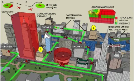
Figure 1.1: Multiple autonomous drone missions in an urban environment.

With autonomous systems no longer restricted to the sterile environments, the problem of their safe planning, i.e. generating trajectories that satisfy given mission requirements, and control, i.e. actuating the dynamical system to follow the desired trajectory, is now one of utmost importance. From self-driving cars, to underwater robots, to multi-rotor drones, autonomous robotic systems are finding widespread applications with complex operating requirements, creating new safety concerns along with them.

(20)

and infrastructure monitoring. Drone A is tasked with delivering a package, which it has to do within 15 minutes and then return to base in the following 10 minutes. Drone B is tasked with periodic surveillance and data collection of the wildlife in the park, while Drone C is tasked with collecting sensor data from equipment on top of the white-and-blue building. All of these missions have complex spatial requirements (e.g. avoid flying over the buildings highlighted in red, perform surveillance or monitoring of particular areas and maintain safe distance from each other), temporal requirements (e.g., a deadline to deliver package, periodicity of visiting the areas to be monitored) and reactive requirements (like collision avoidance).

The scenario outlined in the above example is now close to being a reality. In the United States of America, the National Aeronautics and Space Association (NASA) and the Federal Aviation Authority (FAA) have been studying the regulation of the airspace when multiple fleets of autonomous drones share the same airspace, out-lined in the Concept of Operations document (ConOps) Federal Aviation Authority [2018]. While their focus is on the infrastructure and management of the airspace, the Unmanned Aerial Systems (UAS) Traffic Management (UTM) ConOps makes it clear that the safety (separation from other aircraft, terrain, and other hazards) is a responsibility of the drone fleet operators. The ConOps also outline a potential airspace reservation based system for operation where operators reserve a volume of the airspace for a given time interval to operate in. This approach is no doubt conservative, and will not scale as the airspace gets more crowded.

In fact, the problem of planning for multiple aerial vehicles in the same airspace is not an entirely new one. Air Traffic Control (ATC) operations worldwide guide manned commercial aircrafts from their source to destination while maintaining safety. ATC relies on human controllers to guide aircrafts along pre-designed routes while scheduling/directing operations in a way that maintains separation between aircrafts. Given the number of UAS expected to operate in urban airspaces in the near future, as well as the short time frames of the missions and communication constraints, it is impossible to have humans operators for UTM operations. This motivates the need to have an mission planning system similar to ATC, but for UTM operations.

In UTM operations, each UAS will not be simply going from a source to a destina-tion but may in fact be performing a complicated set of tasks, often working together with multiple other UAS, e.g. in disaster management Homola et al. [2018]. This necessitates that the UTM framework be capable to taking into account complicated mission requirements beyond point to point navigation, as well as be able to handle multiple UAS sharing the same airspace at the same time.

(21)

planned trajectories to within a given tracking error bound.

We aim to take into account these requirements and develop planning and control methods for safe operation of autonomous systems.

1.1 Challenges in planning and control of autonomous

systems

In order to deal with complicated missions requirements, as those outlined in Ex-ample 1.1, most existing approaches either lack the expressiveness to handle such requirements e.g. Ma et al. [2016], van den Berg and Overmars [2015] , rely on sim-plifying assumptions that result in conservative or infeasible behavior Aksaray et al. [2016], or do not take into account the explicit timing requirements Saha et al. [2014]. In addition to these limitations, many of the planning methods are computationally intractable (and hence do not scale well or work in real-time), and provide guarantees only on a simplified abstraction of the system behavior Aksaray et al. [2016]. This leads to the additional problem that plans/trajectories generated by the planning methods may in practice be impossible for the real dynamical system to follow Kan-taros and Zavlanos [2018]. A detailed review of existing approaches is presented in Sec. 8.2.

Despite robot planning and control being a well studied in literature Elbanhawi and Simic [2014],Yang et al. [2016], dealing with the complicated requirements, e.g. those of Example 1.1 pose a fundamental problem due to:

1. Explicit temporal constraints: Asking a dynamical system to satisfy a particular task in some given interval of time adds challenges that are not well studied in literature outside of temporal logic based planning/control (see chap. 8 for more details). Most multi/single-robot planning algorithms either ignore time bounds or aim to achieve the minimum time to completion Guo and Parker [2002], which may not be well suited to a particular application.

2. Multi-agent co-operation across tasks: Planning for multiple agents when they have to perform tasks in a dependent manner adds another layer of complexity. Common approaches to solving these problems either impose task priorities De-wangan et al. [2017] or rely on other heuristics to simplify the problem,possibly at the cost of sacrificing performance.

(22)

4. Disconnect between planing and control: Classical planning methods likeA∗rely on a discrete representation of the workspace and result in jagged trajectories that later need to be smoothed out for an actual dynamical system to follow them. As the safety guarantees are on the original trajectory only, the smoothed trajectory may be unsafe.

5. Robust control with perception based estimation: The problem of control for trajectory following under uncertainty, while well studied, rarely takes into ac-count the impact of the computation time or energy taken to generate a state estimate from a perception (e.g. vision, lidar-based) driven estimator. This can, in practice result in poor control performance and reduced operating time for a robot.

The research presented here aims to develop computationally tractable algorithms that also provide performance guarantees in order to address the above issues.

1.2 Contributions of this work

The research carried out, in order to deal with some of the challenges outlined above, can be divided into two categories.

1. Multi-agent planning with Signal temporal logic (STL) objectives.

This part focuses on generating trajectories for autonomous robots such that they satisfy objectives specified using STL.

2. Robust predictive control with anytime perception. The second part focuses on predictive control algorithms to follow the trajectories generated by our planning methods while staying within a predefinedrobustness tube around the desired trajectory. We explicitly take into account the time and energy consumption of perception-based estimation algorithms that give us state esti-mation as feedback, and show that we do not always need the best quality state estimate to perform the control task. By varying the quality and resource con-sumption of the state estimator online, the control schemes we develop result in improved control performance while being efficient with regards to the energy consumed by the computation.

1.2.1 Connection between the two themes

In Chapter 4, we present a method that generates trajectories for fleets of multi-rotor drones such that they satisfy STL specifications. Along with the trajectories, the

(23)

Multi-agent planning w/ TL speciﬁcations

Robust predictive control w/ Anytime perception

Smooth Operator:

Predictive control with MTL speciﬁcations

Fly-by-Logic:

Drone planning with STL speciﬁcations

Distributed planning for multi-rotor ﬂeets

Co-operative distributed control for collision avoidance MTL/STL Robustness and its smooth

approximation

Trajectories and bounds within which to track

Anytime algorithms for perception driven estimation

Robust Adaptive Model Predictive Control (RAMPC)

Stochastic Adaptive Model Predictive Control (SAMPC)

CPU-GPU co-design for energy/time trade-off in perception based algorithms

Robust Linear MPC for non-linear systems via FB linearization Bounds on

controller performance

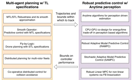
Figure 1.2: Organization of the research contributions of this work. Chapters 3 and 4 address the problem of planning and control with temporal logic objectives, while chapters 6 and 7 address the robust predictive control problem.

show the time-varying sets in which the position of the two quadrotors should be within at the corresponding time step, in order to satisfy the STL specification.

This problem of following the trajectory within given bounds is explored in chap. 6, where we develop a method that does this while also taking into account the be-havior of the perception-based estimator that supplies the state-feedback for the con-troller. The robust adaptive model predictive control algorithm (RAMPC) presented in that chapter takes as reference the trajectories to track as well as the constraints within which to track them (see fig. 1.3) from the planning method. The planning method on the other hand takes into account a characterization of the region within which the controller can track well (see def. 4.1).

1.3 Organization of the document

(24)

specifications. Chapter 4 covers Fly-by-Logic, a method to generate trajectories for multiple multi-rotor UAS such that they satisfy a given STL specification. Chapter 5 presents a user-interface for multi-rotor UAS fleet planning and the briefly covers the underlying tool-chain.

Chapter 6 presents an approach to design a Robust Adaptive Model Predictive Control (RAMPC) algorithm that we use for trajectory tracking. The RAMPC algo-rithm ensures that the dynamical system remains feasible with respect to state and input constraints despite estimation errors and computation delays due to perception-based estimation algorithms. It also leverages a co-design between the computation and control to provide good control performance as well as computation energy con-sumption compared classical MPC approaches that do not. Chapter 7 presents a feedback linearization-based Robust Model Predictive Control method that can al-low the co-design framework to be directly extended to non-linear (control-affine) systems.

(25)

-5

0 x

0 -5

y

z

5

0

5

(26)

Chapter 2 Representing mission requirements

in temporal logic

In this document, the problem of multi-agent planning is studied through the lens of planning with missions given in temporal logic form. This chapter covers the basics of a class of temporal logic that we are interested in, as well as the concept ofrobustness

that is central to the methods presented in the following chapters. Consider a discrete-time dynamical system H given by

xt+1 =f(xt, ut) (2.1)

wherex∈X ⊂_Rn_{is the state of the system and}_u_∈_U _⊂

Rmis its control input. The

system’s initial state x0 takes value from some initial set X0 ⊂ Rn. Given an initial

state x0 and a finite control input sequence u = (u0, . . . , uT−1), ut ∈ U, a trajectory

of the system is the unique sequence of statesx= (x0, . . . , xT) s.t. for all t,xt is inX

and obeys (2.1). All temporal intervals that appear here are implicitly discrete-time, e.g. [a, b] means [a, b]∩_N. The set {0,1, . . . , T} ⊂ _N will be abbreviated as _T. For an intervalI ⊂_N, let t+I ={t+a|a ∈I}. The set of subsets of a setS is denoted

P(S). The signal space XT _{is the set of all signals}_x_:

T→X. The max operator is

writtent and min is written u.

2.1 Metric Temporal Logic (MTL)

The controller ofH is designed to make the closed loop system (2.1) satisfy a specifi-cation expressed in MTL Ouaknine and Worrell [2008]. Formally, let AP be a set of atomic propositions, which can be thought of as point-wise constraints on the state of the system. An MTL formula ϕ is built recursively from the atomic propositions using the following grammar:

(27)

where I ⊂ _R is a time interval. Here, > is the Boolean True, p is an atomic propo-sition, ¬ and ∧ are the Boolean negation and AND operators, respectively, and U

is the Until temporal operator. Informally, ϕ1UIϕ2 means that ϕ1 must hold until

ϕ2 holds, and that the hand-over from ϕ1 to ϕ2 must happen sometime during the

interval I. The disjunction (∨), implication ( =⇒ ), Always () and Eventually (_♦) operators can be defined using the above operators.

Formally, the pointwise semantics of an MTL formula define what it means for a system trajectoryx to satisfy the formulaϕ. LetO :AP → P(X) be an observation

map for the atomic propositions. The boolean truth value of a formula ϕ w.r.t. the trajectory xat time t is defined recursively.

Definition 2.1 (MTL semantics).

(x, t)|=> ⇔ >

∀p∈AP,(x, t) |=O p ⇔ xt∈ O(p)

(x, t)|=O ¬ϕ ⇔ ¬(x, t)|=O ϕ

(x, t)|=O ϕ1 ∧ϕ2 ⇔ (x, t)|=O ϕ1∧(x, t)|=O ϕ2

(x, t)|=O ϕ1UIϕ2 ⇔ ∃t0 ∈t+I.(x, t0)|=O ϕ2 ∧∀t00 ∈(t, t0), (x, t00)|=O ϕ1

As O is fixed here, it is dropped from the notation. We say x satisfies ϕ if (x,0)|=ϕ. All formulas that appear here have bounded temporal intervals: 0≤infI <

supI <+∞. To evaluate whether such a formula ϕholds on a given trajectory, only a finite-length prefix of that trajectory is needed. Its length can be upper-bounded by thehorizon of ϕ, hrz(ϕ)∈_N, calculable as shown in Dokhanchi et al. [2014]. For example, the horizon of [0,2](♦[2,4]p) is 2+4=6.

2.1.1 Robust semantics of MTL

Designing a controller that satisfies the MTL formula ϕ1 is not always enough. In a dynamic environment, where the system must react to new unforeseen events, it is useful to have a margin of maneuverability. That is, it is useful to control the system such that we maximize our degree of satisfaction of the formula. When unforeseen events occur, the system can react to them without violating the formula. This degree of satisfaction can be formally defined and computed using the robust semantics of MTL. Given a point x ∈ X and a set A ⊂ X, dist(x, A) := inf_a_∈_A|x−a|2 is the

minimum Euclidian distance from xto the closure A of A.

Definition 2.2(RobustnessFainekos and Pappas [2009]). Therobustness ofϕrelative

(28)

tox at timet is recursively defined as

ρ>(x, t) = +∞

∀p∈AP, ρp(x, t) =

dist(xt, X \ O(p)), if xt ∈ O(p)

−dist(xt,O(p)), if xt ∈ O/ (p) ρ¬ϕ(x, t) = −ρϕ(x, t)

ρϕ1∧ϕ2(x, t) = ρϕ1(x, t)uρϕ2(x, t)

ρϕ1UIϕ2(x, t) = tt0∈t+TI

ρϕ2(x, t

0

)l

ut00_∈_[_t,t0₎ρ_ϕ

1(x, t

00

)

When t = 0, we writeρϕ(x) instead of ρϕ(x,0).

The robustness is a real-valued function of x with the following important prop-erty.

Theorem 2.1. Fainekos and Pappas [2009] For any x∈XT _{and MTL formula}_ϕ_{, if}

ρϕ(x, t)< 0 then x violates the spec ϕ at time t, and if ρϕ(x, t) >0 then x satisfies ϕ at t. The case ρϕ(x, t) = 0 is inconclusive.

Thus, we can compute control inputs by maximizing the robustness over the set of finite input sequences of a certain length. The obtained sequence u∗ is valid if

ρϕ(x, t) is positive, where x and u∗ obey (2.1). The larger ρϕ(x, t), the more robust

is the behavior of the system: intuitively, xcan be disturbed and ρϕ might decrease

but not go negative.

2.2 Signal Temporal Logic (STL)

In chapter 4 we present a method for multi-rotor drone fleet planning with mission specifications expressed in Signal Temporal Logic (STL) Maler and Nickovic [2004], Donz´e and Maler [2010b]. Similar to MTL, STL is a logic that allows the succinct and unambiguous specification of a wide variety of desired system behaviors over time, such as “The quadrotor reaches the goal within 10 time units while always avoiding obstacles” and “While the quadrotor is in Zone 1, it must obey that zone’s altitude constraints”.

Formally, let M ={µ1, . . . , µL} be a set of real-valued functions of the state µk : X → _R. For each µk define the predicate pk :=µk(x) ≥ 0. Set AP := {p1, . . . , pL}.

Thus each predicate defines a set, namely pk defines {x∈X |fk(x)≥0}. Similar to

MTL, let I ⊂_R denote a non-singleton interval, > the Boolean True, p a predicate,

¬ and ∧ the Boolean negation and AND operators, respectively, and U the Until temporal operator. An STL formula ϕis built recursively from the predicates using the following grammar:

(29)

2

1

3

4 Unsafe

₁

Unsafe

₂

Goal

Figure 2.1: This illustration shows a UAS and two trajectories, x1 (in black) and x2 (in

blue). Color in digital version.

2.2.1 Robustness of STL specifications

STL follows the same grammar as that of MTL and has similarly defined robust semantics as well (see 2.1.1). The notable difference is that thedistoperator in MTL for each predicate pk is simply replaced by µk in STL, where µk is the real-valued

function that defines the predicate pk as described above. This means that the only

difference with respect to definition 2.2 is that ρp(x, t) =µ(xt), where xt is the value

of signal xat timet. The rest of the robust semantics of STL follow the construction of definition 2.2.

The STL specifications we consider in the rest of this document satisfy the fol-lowing assumption:

Assumption 2.1. The function µ that defines an atomic proposition in STL is con-tinuously differentiable, or µ∈C1_.

The following shows an example of a specification in STL and its associated ro-bustness:

Example 1. Consider a safety specification of the form:

(30)

2.1 shows these regions. Consider the trajectory x1 (in black), shown from time 0 to

T seconds. As can be seen, the UAS does indeed avoid the unsafe regions and satisfies the specification, which by Theorem 2.1 implies that the robustness of this trajectory x with respect to the specification ϕsafe, ρϕsafe(x) is positive.

In order to further understand this robustness value, let us first compute it. Let

p = [px, py] be the position of the drone in 2-d. The proposition p ∈ Unsafe1 can be written in more detail in STL as (px ≤ −1)∧(−px ≤ 2)∧(py ≤ 2)∧(−py ≤ −1).

This comes from the representation of the set as a bounded axis-aligned polyhedron in _R2. Following the robustness semantics of definition 2.2 that states the robustness

ρϕ1∧ϕ2 = min(ρϕ1, ρϕ2), the robustness ofp∈Unsafe, evaluated at a single point in the

trajectory, can be computed asρUnsafe1(p) = min(−1−px, 2 +px, 2−py, −1 +py). As

an example, consider the point [−1.5,0.75]0 marked by 1 in fig. 2.1. The robustness of this point w.r.t proposition p ∈ Unsafe₁ is ρUnsafe1 = min(0.5, 0.5,1.25,−0.25) =

−0.25. This negative robustness implies that the point [−1.5,0.75]0 does not satisfy the proposition p∈Unsafe₁, which is as seen in the figure.

Since a part of the safety specification ϕsafeasks for¬(p∈Unsafe1), the robustness of this proposition is simply the negative of the robustness of the proposition p ∈ Unsafe₁ (again see def. 2.2), or 0.25.

To then evaluate the robustness of [0,T]¬(p ∈ Unsafe1), following def. 2.2, we need to compute the minimum of the robustness of the proposition ¬(p ∈ Unsafe₁)

over all points from time 0to T in trajectory x1, i.e. mint∈[0,T](−min(−1−px(t), 2 + px(t), 2−py(t), −1 +py(t))). For trajectory x1, this minimum is achieved by the point

marked by 1, hence the robustness of trajectory x1 w.r.t the specification [0,T]¬(p∈ Unsafe₁)is0.25. Similarly we can compute the robustness of the specification[0,T]¬(p∈ Unsafe₂). The robustness of the safety specification ϕsafe is then (using ρϕ1∧ϕ2 = min(ρϕ1, ρϕ2)) given by minimum of the robustness of [0,T]¬(p ∈ Unsafe1) and

[0,T]¬(p∈Unsafe2). For the trajectoryx1, this value is achieved by the point marked by 1, and is hence 0.25.

This value of 0.25 implies that each point in the trajectoryx1 could be moved by

at most 0.25m along any axis and still the trajectory would satisfy the specification

ϕsafe. Again, focusing on the point marked by 1 helps explain this. If we move 1

along the y-axis by upto 0.25m, 1 still does not enter the set Unsafe1. By moving

(31)

Chapter 3 Smooth Operator: Control with

Temporal Logic Objectives

3.1 Introduction: Controlling for robustness

The errors in a cyber-physical control system like an automated air traffic controller can affect both the cyber components (e.g., software bugs) and physical components (e.g., sensor failures and attacks) of a system. Under certain error models, like a bounded disturbance on a sensor reading, a system can be designed to be robust to that source of error. In general, however, unforeseen and unmodeled issues will occur and the controller has to deal with them at runtime. To help deal with unforeseen problems at runtime, the system’s controller must make decisions that not only satisfy the system’s requirements (like a maximum response time to an event), but satisfy them robustly. Intuitively, the requirements are robustly satisfied if a disturbance to the system does not cause it to violate them. This can give a margin of maneuvara-bility to the system during which it addresses the unforeseen problem. Since these problems are, by definition, unforeseen and unmodeled and only detected by their effect on the output, the notion of robustness must be computable using only the output behavior of the system.

Example 2. Air-Traffic Control (ATC) coordinates landing arrivals at an airport. ATCs have very complex rules to ensure that all airplanes, of different sizes and speeds, approach the airport and land safely, with sufficient margin to other airplanes to accommodate emergencies. Sample rules for the Chicago O’hare airport include (A) When an aircraft enters any of 3 designated zones, it must stay between that zone’s altitude floor and ceiling, and (B) If the airspace is too busy, an aircraft must remain in either holding zones 6 or 7, until some maximum amount of time expires.

(32)

3.1.1 The need for temporal logic

The above requirements go beyond traditional control objectives like stability, track-ing, quadratic cost optimization and reach-while-avoid for which we have well-developed theory. While these requirements can be directly encoded from natural language into a Mixed Integer Program (MIP) by encoding every possibility at each (discrete) time point with integer variables, such a direct encoding can easily involve an exorbitant number of variables. For complex requirements, with many variables involved, this encoding process can also be error-prone and checking that it corresponds to the designer’s intent is near impossible. On the other hand, such control requirements are easily and succinctly expressed in Metric Temporal Logic (MTL) Ouaknine and Worrell [2008]. MTL is a formal language for expressing reactive requirements with constraints on their time of occurrence and sequencing, such as those of the ATC (see chapter 2). The advantage of first expressing the requirements in MTL is that MTL formulas are more succinct and legible, and less error-prone, than the corresponding directly-encoded MIP. In this sense, MTL bridges the gap between the ease of use of natural language and the rigour of mathematical formulation. For example, ATC rule (A) can be formalized with the following MTL formula ( means ‘Always’, q is an aircraft andqz is its altitude).

(q ∈Zone1 =⇒ qz ≤Ceiling1∧qz≥Floor1)

Rule (B) can be formalized as follows.

(Busy =⇒ ♦[t1,t2](q∈Holding-6 ∨ q∈Holding-7)U[0,MaxHolding]¬Busy)

This says that Always (), if airport is Busy, then sometime t1 tot2 seconds later

(_♦[t1,t2]), the plane goes into one of two Holding areas. It stays thereUntil the airport is not (¬) busy, which must happen before duration MaxHolding elapses.

Given an MTL specification ϕand a system execution x, the robustness ρϕ(x) of

the spec relative to x measures two things: its sign tells whether xsatisfies the spec (ρϕ(x) >0) or violates it (ρϕ(x)< 0). Its magnitude |ρϕ(x)| measures how robustly

the spec is satisfied or violated. Namely, any perturbation to x of size less than

|ρϕ(x)| will not cause its truth value to change relative to ϕ. Thus, we are interested

in developing a control algorithm that can maximize the robustness over all possible control actions to determine the next control input.

Unfortunately, the robustness function ρϕ is hard to work with. In particular, it

(33)

function classes, usually have a fewer number of parameters to be set, and important issues like step-size selection are rigorously addressed.

Contributions. This chapter presents smooth (infinitely differentiable) tions to the robustness function of arbitrary MTL formulae. The smooth approxima-tion is proven to always be within a user-defined error of the true robustness, and this is illustrated experimentally. This allows running powerful and rigorous off-the-shelf gradient descent optimizers. We leverage this to maximize the smooth robustness for control of a system to robustly satisfy its MTL specification. Through multiple examples, the proposed control method is shown to be faster and to yield more robust trajectories than various current heuristics and MIP-based approaches. The results are demonstrated on a case study for an autonomous ATC for two quad-rotors, where the MIP-based approach fails to yield a satisfying controller. While this work does not tackle the non-convexity of MTL robustness issue directly, having an inexpen-sive gradient optimizer makes it possible to run an efficient multi-start optimization, increasing the chances of approaching the global optimum.

3.2 Smooth approximation of MTL Robustness for

Control

Let ϕbe an MTL formula with horizon N. The goal of the present work is to solve the following problem Pρ.

Pρ : max

u ρϕ(x)−γ

N−1

X

k=0

l(xk+1, uk) (3.1a)

s.t. xk+1 =f(xk, uk), ∀k = 0, . . . , N −1 (3.1b)

xk ∈X, ∀k= 0, . . . , N (3.1c)

uk ∈U,∀k = 0, . . . , N −1 (3.1d)

δρϕ(x)≥δmin (3.1e)

Here, u= (u0, . . . , uN−1),l(xk+1, uk) is a control cost, e.g. the LQR costx0kQxk+ u0_kRuk, andγ ≥0 is a trade-off weight. The scalar min ≥0 is a desired minimum

ro-bustness. Ifδ = 0, then this constraint is effectively removed, whileδ = 1 enforces the constraint. Because ρϕ uses the non-differentiable functions dist, max and min (see

definition 2.2), it is itself non-differentiable. The next three sub-sections introduce smooth approximations to each of these functions.

Assumption 3.1. The function f : _Rn×_Rm _→

Rn that represents the system

(34)

3.2.1 Approximating the distance function

The distance function dist(·, U) is in L2(Rn), so it can be approximated arbitrarily

well using a Meyer wavelet expansion DeVore [1998]. Specifically, the 1-D Meyer wavelet function is given in the frequency domain by (i=√−1):

b

ψ(ω) = √1

2π 





sin(π₂ν(3₂|ω_π|−1))eiω/2 ₂_π/₃_{≤ |}_ω_{| ≤}₄_π/₃

cos(π₂ν(3₄|ω_π|−1))eiω/2_, ₄_π/₃_{≤ |}_ω_{| ≤}₈_π/₃

0, otherwise

where ν(x) = 0 if x ≤ 0, 1 if x ≥ 1, and equals x if 0 ≤ x ≤ 1. The time-domain expression for this wavelet is given in Vermehren Valenzuela and de Oliveira [2015] and is infinitely differentiable. Ann-D wavelet can be obtained using the tensor product construction DeVore [1998]. LetE be the set of vertices of the unit hypercube [0,1]n_.

For every e = (e1, e2, . . . , en)∈E and x= (x1, . . . , xn)∈Rn, define Ψe :Rn →R by

Ψe(x) = ψe1₍_x

1). . . ψen(xn). Given k ∈ Z and j ∈ Zn, a dyadic cube in Rn is a set

of the form I = 2−k₍_j_{+ [0}_,_1]n_{). Let} _D _{be the set of all dyadic cubes in}

Rn obtained

by varyingk over_Z and jover _Zn_{. Then}_{_Ψe

I, e∈E, I ∈D} is an orthonormal basis

forL2(Rn) (because the Meyer wavelet itself is orthonormal). Then every function in

L2(Rn) has an expansion

f(x) = X

I∈D X

e∈E

ce_IΨe_I(x), ce_I := hf,Ψe_Ii

with hh, gi :=R

Rnh(x)g(x)dx. The desired approximation is obtained by truncating

this expansion after a finite number of terms, i.e., by using a finite setD0 ₍D

dist(x, U)≈distg_ε(x, U) := X

I∈D0

X

e∈E

ce_IΨe_I(x) (3.2)

whereεis the approximation error magnitude. Using more coefficients yields a better approximation. The coefficientsce_I := hdist(·, U),Ψe_Iiare calculated offline and stored in a lookup table for online usage.

3.2.2 Smooth max and min

The following standard smooth approximations of m-ary max and min are used. Let

k ≥1.

g

maxk(a1, . . . , am) :=

1

k ln(e

ka1 ₊_{. . .}₊_ekam₎ _(3.3)

g

mink(a1, . . . , am) := −max(g −a1, . . . ,−am) (3.4)

Suppose k = 1 and that a1 is the largest number. Then ea1 is even larger than the

other eai_{’s, and dominates the sum. Thus}

g

(35)

not significantly larger than the rest, the sum is not well-approximated byea1 _alone. To counter this, the scaling factor k is used: it amplifies the differences between the numbers. It holds that for any set of m reals,

0≤max_gk(a1, . . . , am)−max(a1, . . . , am)≤ln(m)/k (3.5)

0≤min(a1, . . . , am)−mingk(a1, . . . , am)≤ln(m)/k (3.6)

with the maximum error is achieved when all the ai’s are equal. Indeed, assume a1

is the largest number, then max_gk(a)−a1 ≤k−1ln

P iekai

eka₁

≤lnm/k.

3.2.3 Overall approximation

Putting the pieces together yields the approximation error for the robustness of any MTL formula.

Theorem 3.1. Consider an MTL formula ϕ and reals ε > 0 and k ≥ 1. Define the smooth robustness ρ˜ϕ, obtained by substituting distg_ε for dist,

g

maxk formax, and g

mink for min, in Def. 2.2. Then for any trajectory x, it holds that

|ρϕ(x, t)−ρ˜ϕ(x, t)| ≤δϕ

where δϕ is (a) independent of the evaluation time t, and (b) goes to 0 as ε→0 and k → ∞.

Proof. We will prove a stronger result that implies the theorem. When x or t are clear from the context, we will drop them from the notation.

The proof is by structural induction on ϕ, and works by carefully characterizing the approximation error.

Case ϕ=p∈AP. ρϕ(x, t) is given by either distxtO(p) or −distxtO(p), and

˜

ρϕ(x, t) is given by either distgε(xt,O(p)) or −distgε(xt,O(p)), respectively. Either

way, |ρ˜ϕ(x, t)−ρϕ(x, t)| ≤ε. Indeed, ε satisfies the conditions on δϕ.

Case ϕ=¬ϕ1 |ρ¬ϕ1(x, t)−ρ˜¬ϕ1(x, t)| = | −ρϕ1(x, t) + ˜ρϕ1(x, t)| ≤ δϕ1, and δϕ1 satisfies (a)-(b) by the induction hypothesis.

Case ϕ=ϕ1∨ϕ2. If the same sub-formulaϕi achieves the max for bothρϕ1(x, t)t

ρϕ2(x, t) and ˜ρϕ1(x, t)tρ˜ϕ2(x, t), then by induction hypothesis we immediately obtain

|ρϕ(x, t)−ρ˜(x, t)| ≤δϕi.

Otherwise if, say, ρϕ =ρϕ1 and ˜ρϕ = ˜ρϕ2 then

ρϕ1 −δϕ1 ≤ρ˜ϕ1 ≤ρ˜ϕ2 =⇒ ρϕ1 −ρ˜ϕ2 ≤δϕ1

Also

˜

ρϕ2 ≤ρϕ2 +δϕ2 ≤ρϕ1 +δϕ2 =⇒ −δϕ2 ≤ρϕ1 −ρ˜ϕ2

Therefore

(36)

Similarly, if ρϕ =ρϕ2 and ˜ρϕ = ˜ρϕ1, we have |ρϕ2−ρ˜ϕ1| ≤δϕ1 tδϕ2. So in all cases,

|ρϕ1 tρϕ2 −ρ˜ϕ1 tρ˜ϕ2| ≤δϕ1tδϕ2

Therefore by the triangle inequality and (3.5)

|ρϕ1 tρϕ2 −maxgk( ˜ρϕ1,ρ˜ϕ2)| ≤δϕ1 tδϕ2 + ln(2)/k =δϕ

Clearly,δϕ satisfied (a)-(b).

The case ϕ1∧ϕ2 is treated similarly.

ϕ=ϕ1UIϕ2. Before proving this case, we will need the following lemma, which is

provable by induction on n:

Lemma 1. If ϕ = ϕ1 ∧. . .∧ϕn or ϕ = ϕ1 ∨. . .∨ϕn, n ≥ 2, then |ρϕ −ρ˜ϕ| ≤

t1≤i≤nδϕi+ ln(n)/k.

We now proceed with the proof of the last case. Recall that ρϕ1UIϕ2(x, t) =

tt0_∈_t₊

TI(ρϕ2(x, t

0

)d

ut00_∈_[_t,t0₎ρ_ϕ

1(x, t

00₎

. Starting with the innermost sub expressionρψ :=ut00_∈_[_t,t0₎ρ_ϕ

1(x, t

00_),

we have, by Lemma 1

|ρψ −ρ˜ψ| ≤ tt00_∈_[_t,t0₎δt 00

ϕ1 + ln(t

0₋_t₎_/k _(3.7)

where δt00

ϕ1 is the bound for approximating ρϕ1(x, t

00_{). But}_δ

ϕ does not depend on the

time at which the formula is evaluated. Therefore the bound in (3.7) becomes

|ρψ −ρ˜ψ| ≤δϕ1 + ln(t

0₋

t)/k (3.8)

To avoid introducing a dependence on time, we further upper-bound by

|ρψ−ρ˜ψ| ≤δϕ1 + ln(hrz(ϕ))/k :=δψ

where, recall, hrz(ϕ) is the horizon of ϕ(see Section 2.1). Continuing with the sub-expressionρα =ρϕ2(x, t

0₎d

ρψ, by the induction

hypoth-esis it holds that |ρα −ρ˜α| ≤ δϕ2 tδψ + ln(2)/k := δα. Finally, the top-most max operator introduces the total error

|ρϕ−ρ˜ϕ| ≤ δα+ ln(|I|)/k

= δϕ2 tδψ + ln(2)/k+ ln(|I|)/k

= δϕ2 t(δϕ1 + ln(hrz(ϕ))/k) + ln(2|I|)/k

= δϕ (3.9)

The first inequality obtains from the fact that δα is independent of evaluation time

(37)

3.2.4 The need for smoothing

The application of gradient descent methods requires a differentiable objective func-tion. Our objective function, ρϕ, is non-differentiable, because it uses the distance,

max, and min functions, all of which are non-differentiable. One may note that these functions are all differentiable almost everywhere (a.e.) on their domain. That is, the set of points in their domain where they are non-differentiable has measure 0 in _Rn_.

Therefore, by measure additivity, the composite functionρϕ is itself differentiable a.e.

Thus, one may be tempted to ‘ignore’ the singularities (points of non-differentiability), and apply gradient descent to ρϕ anyway. The rationale for doing so is that sets of

measure 0 are unlikely to be visited by gradient descent, and thus don’t matter. However, as we show in the next example, the lines of singularity (along which the objective is non-differentiable) can be precisely the lines along which the objective increases the fastest. See also Cortes [2008]. Thus they are consistently visited by gradient descent, after which it fails to converge because of the lack of a gradient.

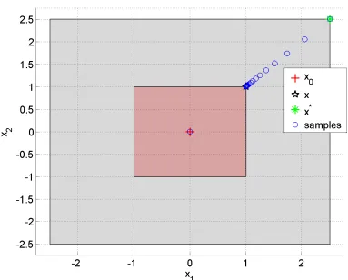
Example 3. A simple example illustrates how gradient descent gets stuck at singular-ities. We use the optimization algorithm Sequential Quadratic Programming (SQP) Polak [1997] to maximize the robustness of ϕ=¬(x∈U), where U = [−1,1]2 _{is the} unsafe red square in Fig. 3.1. In this case, ρϕ is simply dist(x0, U), the distance of the first trajectory point to the set. The search space is [−2.5,2.5]2 (big grey square in Fig. 3.1). The most robust points are the corners of the grey square, such as

x∗ = [2.5,2.5] (green ‘+’ in figure), being furthest from the unsafe set. We initialize the SQP at x0 = [0,0]. SQP generates iterates (blue circles) on the line of singularity connecting [1,1]to x∗ and ultimately gets stuck atx= [1,1]. That’s because along the line, the gradient does not exist and attempts by SQP to approximate it numerically fail, prompting it to generate smaller and smaller step-sizes for the approximation. Ultimately, SQP aborts due to the step-size being too small, and concludes it is at a local minimum.

3.3 Approximation and control

We implemented the smooth approximation to the semantics of MTL, and tested it on several examples.

3.3.1 Approximation error

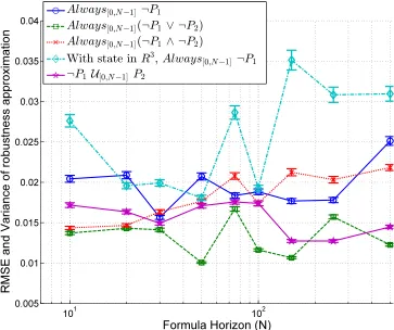
We evaluated the robustnessρϕ and its approximation ˜ρϕ for five formulae. The

hori-zon N of each formula is varied, and at each value ofN we generate 1000 trajectories of systemxk+1 =xk+uk with input and state saturation, by feeding it random input

sequences. Fig. 3.2 shows the Root Mean Square (RMSE) of the approximation,

p

(1/1000)P

x(ρϕ(x)−ρ˜ϕ(x))2, and variance bars around it. As seen, the

(38)

Figure 3.1: Iterates of SQP for Example 3. Colors in online version.

the smooth approximation. Note that while the RMSE increased with the system dimension (4th _{formula in Fig. 3.2), it was observed that the relative error remained}

very small i.e. the increase in error is explained by an increase in the robustness’s magnitude.

3.3.2 Robustness maximization for control

ProblemPρ given in (3.1) is solved by replacing the true robustness ρϕ by its smooth

approximation ˜ρϕ, and setting min to the value of the smooth approximation error.

We thus obtain Problem Pρ˜. This approach is labeled Smooth Operator (SOP). Optimization solver. Problem Pρ˜ is solved using Sequential Quadratic

(39)

101 102 0.005 0.01 0.015 0.02 0.025 0.03 0.035 0.04

Formula Horizon (N)

R M S E a n d V a ri a n c e o f ro b u s tn e s s a p p ro x im a ti o n

Always_[0,N!1] ¬P1

Always_[0,N!1](¬P1 ∨ ¬P2)

Always_[0,N!1](¬P1 ∧ ¬P2)

With state in R3,Always_[0,N!1] ¬P1

¬P₁ U_[0_,N

!1] P2

Figure 3.2: Robustness approximation error against formula horizon, evaluated on 1000 randomly generated trajectories for Example 4. Unless noted, the systems are 2D. Color in online version.

lie on the boundary of the inequality-feasible set there exists a search direction towards the interior of the feasible set that does not violate the equality constraints [Polak 1997, Assumption 2.9.1]. This is also true for Pρ˜ since the equality constraints come

from the dynamics and are always enforced for any u.

Solver initialization. To initialize SQP when solvingPρ˜(i.e., to give it a starting

value for u), we can either solve an inexpensive feasibility linear program with con-straints (3.1b)-(3.1d), or generate a random input sequence respecting ut ∈ U. The

resulting initial trajectory could violate the specification (as it does in every example we study here) and it is only required to satisfy the dynamics and state constraints.

Comparisons to BluSTL.The tool BluSTL implements the MILP approach of Raman et al. [2014] and is used in the experiments. It has two modes of operation: mode (B) or Boolean, which aims at satisfying the specification without maximizing its robustness, and mode (R) orRobust, which attempts to maximize robustness. The proposed SOP method optimizes robustness and so naturally runs in mode (R). SOP emulates mode (B) by terminating the optimization as soon as ˜ρϕ ≥ Meyer, which

implies ρϕ ≥ 0. Meyer can be computed explicitly using the approach in the online

(40)

Table 3.1: Example 4. Runtimes (mean and standard deviation, in seconds) for Smooth Operator (SOP) and BluSTL (BlS) in modes (B) and (R), over 100 runs with random initial states and different formula horizons N. BluSTL(R) did not finish (see text).

N BlS(B) SOP(B) BlS(R) SOP(R)

20 0.96±0.82 0.31±0.13 NA 3.30±1.25 30 1.37±1.72 0.33±0.25 NA 5.85±2.74 40 3.86±5.10 0.60±0.29 NA 12.36±6.04 50 4.36±12.97 0.74±0.30 NA 30.05±18.23 100 16.77±27.84 1.21±0.25 NA 69.70±13.16 200 53.88±14.18 4.19±1.18 NA 126.11±20.43

Example 4. The linear system xk+1 =xk+uk is controlled to satisfy the specification ϕ=[0,20]¬(x∈Unsafe)∧♦[0,20](x∈Terminal)

with the sets Unsafe = [−1,1]2 _{and Terminal} _{= [2}_,₂_._5]2_{. The state space is} _X ₌

[−2.5,2.5]2_, _U _{= [}₋₀_.₅_,₀_._5]2_{. Unless otherwise indicated,} _γ ₌ _δ _{= 0} _{in Eq.} _(3.1) _to focus on robustness maximization in this illustrative example. Experiments were run on a quad-core Intel i5 3.2GHz processor with 24GB RAM, running MATLAB 2016b. Results. Fig. 3.3 shows the trajectories of length N = 20 obtained by SOP and BluSTL in modes (B) and (R), starting from the same initial point x0 = [−2,−2]0. Both BluSTL(B) and SOP(B) produce satisfying trajectories. The trajectory from SOP(R) ends in the middle of the terminal set, resulting in a higher robustness than mode (B), as expected. In mode (R), BluSTL could not finish a single instance of robustness maximization within 100 hours on both the above machine and on a more powerful 8 core Intel Xeon machine with 60GB RAM, leading us to believe that the corresponding MILP was not tractable.

SOP(R, γ= 0.1) takes into account a control cost l(xk, uk) =||xk||22 that penalizes longer trajectories. The resulting trajectory is shorter but has a lower robustness than SOP(R, γ = 0), (0.236 vs 0.247).

For further evaluation, we ran 100 instances of the problem, varying the trajec-tory’s initial state in [−2.5,−1.5]×[−2.5,2.5]. We also varied the formula horizon

N (and hence the size of the problem) from20 to200 time steps. Table 3.1 shows the execution times.

Analysis. As seen in Table 3.1, SOP is consistently faster than BluSTL in Boolean mode, and displays smaller variances in runtimes. Note also that the problem solved here is very similar to the one used in Saha and Julius [2016], which uses another MILP-based method. While the underlying dynamics differ and their numbers are reported on a more power machine, SOP numbers compare favourably with those in Saha and Julius [2016].

In (R) mode, across 100 experiments, SOP has an averageρϕ = 0.247 with a

(41)

Figure 3.3: The first 4 trajectories are for Example 4. The last trajectory, SOP(R, unicycle), is from Example 5. Colors in online version.

which is 0.25. This bound is achieved by a trajectory reaching (in <20 time steps) the center of the Terminal set while remaining more than 0.25 distant from Unsafe. Example 5 (Nonlinear system). Since SQP can handle non-linear (twice differen-tiable) constraints, Smooth Operator can also deal with non-linear dynamics whereas the MILP-based methods have to linearize the dynamics to solve the system. The following example shows SOP applied in a one-shot manner to the unicycle dynamics (x˙t = vtcos(θt),y˙t = vtsin(θt),θ˙t = ut) discretized at 10Hz. For the specification

of Ex. 4, the resulting trajectory of length 20 steps obtained by SOP(R) is shown in Fig. 3.3, starting from an initial state of [−2,−2,0]. The resulting robustness is

0.248, which is close to the global optimum of 0.25. This shows that SOP can indeed handle non-linear dynamics without the need for explicit linearization as long as the systems satisfy assumption 3.1.

Safe Planning And Control Of Autonomous Systems: Robust Predictive Algorithms

ScholarlyCommons

ScholarlyCommons

Safe Planning And Control Of Autonomous Systems: Robust

Safe Planning And Control Of Autonomous Systems: Robust

Predictive Algorithms

Predictive Algorithms

Safe Planning And Control Of Autonomous Systems: Robust Predictive

Safe Planning And Control Of Autonomous Systems: Robust Predictive

Algorithms

Algorithms

Acknowledgments

Contents

List of Tables

List of Figures

Chapter 1

Introduction

1.1

Challenges in planning and control of autonomous

systems

1.2

Contributions of this work

1.2.1

Connection between the two themes

1.3

Organization of the document

-5

0

x

0

-5

y

z

5

0

5

5

Chapter 2

Representing mission requirements

in temporal logic

2.1

Metric Temporal Logic (MTL)

2.1.1

Robust semantics of MTL

2.2

Signal Temporal Logic (STL)

2

1

3

4

Unsafe

Unsafe

Goal

2.2.1

Robustness of STL specifications

Chapter 3

Smooth Operator: Control with

Temporal Logic Objectives

3.1

Introduction: Controlling for robustness

3.1.1

The need for temporal logic

3.2

Smooth approximation of MTL Robustness for

Control

3.2.1

Approximating the distance function

3.2.2

Smooth max and min

3.2.3

Overall approximation

3.2.4

The need for smoothing

3.3

Approximation and control

3.3.1

Approximation error

3.3.2

Robustness maximization for control

3.4