R E S E A R C H A R T I C L E
Open Access
Interpreting patient-Specific risk
prediction using contextual decomposition
of BiLSTMs: application to children with
asthma
Rawan AlSaad
1,2*, Qutaibah Malluhi
2, Ibrahim Janahi
3and Sabri Boughorbel
1Abstract
Background: Predictive modeling with longitudinal electronic health record (EHR) data offers great promise for accelerating personalized medicine and better informs clinical decision-making. Recently, deep learning models have achieved state-of-the-art performance for many healthcare prediction tasks. However, deep models lack
interpretability, which is integral to successful decision-making and can lead to better patient care. In this paper, we build upon the contextual decomposition (CD) method, an algorithm for producing importance scores from long short-term memory networks (LSTMs). We extend the method to bidirectional LSTMs (BiLSTMs) and use it in the context of predicting future clinical outcomes using patients’ EHR historical visits.
Methods: We use a real EHR dataset comprising 11071 patients, to evaluate and compare CD interpretations from LSTM and BiLSTM models. First, we train LSTM and BiLSTM models for the task of predicting which pre-school children with respiratory system-related complications will have asthma at school-age. After that, we conduct quantitative and qualitative analysis to evaluate the CD interpretations produced by the contextual decomposition of the trained models. In addition, we develop an interactive visualization to demonstrate the utility of CD scores in explaining predicted outcomes.
Results: Our experimental evaluation demonstrate that whenever a clear visit-level pattern exists, the models learn that pattern and the contextual decomposition can appropriately attribute the prediction to the correct pattern. In addition, the results confirm that the CD scores agree to a large extent with the importance scores generated using logistic regression coefficients. Our main insight was that rather than interpreting the attribution of individual visits to the predicted outcome, we could instead attribute a model’s prediction to a group of visits.
Conclusion: We presented a quantitative and qualitative evidence that CD interpretations can explain patient-specific predictions using CD attributions of individual visits or a group of visits.
Keywords: Interpretability, Deep learning, Predictive models, Electronic health record
Background
The exponential surge in the amount of digital data cap-tured in electronic health record (EHR) offers promis-ing opportunities for predictpromis-ing the risk of potential diseases and better informs decision-making. Recently, deep learning models have achieved impressive results,
*Correspondence:[email protected]
1Machine Learning Group, Sidra Medicine, Doha, Qatar
2Department of Computer Science and Engineering, Qatar University, Doha, Qatar
Full list of author information is available at the end of the article
compared to traditional machine learning techniques, by effectively learning non-linear interactions between fea-tures for several clinical tasks [1–5]. Among a variety of deep learning methods, recurrent neural networks (RNNs) could incorporate the entire EHR to produce predictions for a wide range of clinical tasks [6–11]. Con-sequently, there is a growing realization that, in addition to predictions, deep learning models are capable of pro-ducing knowledge about domain relationships contained in data; often referred to as interpretations [12,13].
However, the high-dimensionality and sparsity of med-ical features captured in the EHR makes it more complex for clinicians to interpret the relative impact of features and patterns which are potentially important in deci-sions. A patient’s EHR usually consists of a sequence of visits a patient has made, and each visit captures the list of diagnosis codes documented by the clinician. Therefore, it is reasonable and important to have inter-pretable models which can focus on patient visits that have higher impact on the predicted outcome, ignore those visits with little effect on the outcome, and iden-tify and validate the relevant subset of visits driving the predictions.
Interpreting deep models trained on EHR data for healthcare applications is a growing field spanning a range of techniques, which can be broadly catego-rized into three classes: attention mechanism, knowledge injection via attention, and knowledge distillation [1]. Attention-mechanism-based learning was used in [14– 20] for explaining what part of historical information weighs more in predicting future clinical events. Knowl-edge injection via attention often integrates biomedi-cal ontologies, as a major source of biomedibiomedi-cal knowl-edge, into attention models to enhance interpretability, as demonstrated in [16]. Knowledge distillation first trains a complex, slow, but accurate model and then com-presses the learned knowledge into a much simpler, faster, and still accurate model, as shown in [21, 22]. However, the majority of previous work has focused on assign-ing importance scores to individual features. As a result, these techniques only provide limited local interpreta-tions and do not model fine-grained interacinterpreta-tions of groups of input features. In addition, most of these techniques require modifications on standard deep learning archi-tectures to make it more interpretable. By contrast, there are relatively few methods that can extract interactions between features that a deep neural network (DNN) learns. In the case of LSTMs, a recent work by Mur-doch et al. [23] introduced contextual decomposition (CD), an algorithm for producing phrase-level impor-tance scores from LSTMs without any modifications to the underlying model, and demonstrated it on the task of sentiment analysis.
In this paper, we hypothesized that the CD interpretabil-ity method translates well to healthcare. Therefore, we build upon the CD technique and extend it to BiLSTMs in the context of predicting future clinical outcomes using EHR data. Particularly, we aimed to produce visit-level CD scores explaining why a BiLSTM model produced a cer-tain prediction using patients’ EHR historical visits. Our main insight was that rather than interpreting the attri-bution of individual visits to the predicted outcome, we could instead attribute BiLSTM’s prediction to a subset of visits. Our main contributions are as follows:
• We introduce a CD-based approach to determine the relative contributions of single visits and a group of visits in explaining the predicted outcome, and subsequently identify the most predictive subset of visits.
• We develop an interactive visualization and demonstrate, using a concrete case study, how CD scores offer an intuitive visit-level interpretation.
• We evaluate and compare CD interpretations from LSTM and BiLSTM models for the task of predicting which pre-school children with respiratory
system-related complications will have asthma at school age.
• On a real EHR dataset comprising 11,071 patients having a total of 3318 different diagnosis codes, we present quantitative and qualitative evidence that CD interpretations can explain patient-specific
predictions using CD attributions of individual visits or a group of visits.
Methods
EHR data description
The EHR data consists of patients’ longitudinal time-ordered visits. Let P denote the set of all the patients
{p1,p2,. . .,p|P|}, where |P| is the number of unique patients in the EHR. For each patient p ∈ P, there areTptime-ordered visitsV1(p),V2(p),. . .,VT(pp). We denote
D = {d1,d2,. . .,d|D|} as the set of all the diagno-sis codes, and |D| represents the number of unique diagnosis codes. Each visit Vt(p), where the subscript t indexes the time step, includes a subset of diag-nosis codes, which is denoted by a vector x(tp) ∈
{0, 1}|D|. The i-th element in x(tp) is 1 if di existed in visit Vt(p) and 0 otherwise. For notational convenience, we will henceforth drop the superscript (p) indexing patients.
Long short term memory networks
Long short term memory networks (LSTMs) are a spe-cial class of recurrent neural networks (RNNs), capable of selectively remembering patterns for long duration of time. They were introduced by Hochreiter and Schmid-huber [24], and were refined and widely used by many people in following work. For predictive modeling using EHR data, LSTMs effectively capture longitudinal obser-vations, encapsulated in a time-stamped sequence of encounters (visits), with varying length and long range dependencies. Given an EHR record of a patient p, denoted byX = {xt}Tt=1, whereTis an integer
it=σ(Wixt+Uiht−1+bi) (1)
ft=σ(Wfxt+Ufht−1+bf) (2)
ot=σ(Woxt+Uoht−1+bo) (3)
gt=tanh(Wgxt+Ught−1+bg) (4)
ct=ftct−1+itgt (5)
ht=ottanh(ct) (6)
Wherei,f, andoare respectively the input gate, forget gate, and output gate, ct is the cell vector, and gt is the candidate for cell state at timestampt,htis the state vec-tor, Wi,Wf,Wo,Wg represent input-to-hidden weights,
Ui,Uf,Uo,Ug represent hidden-to-hidden weights, and
bi,bf,bo,bgare the bias vectors. All the gates have sigmoid activations and cells have tanh activations.
Bidirectional long short term memory networks
Bidirectional LSTMs [25] make use of both the past and the future contextual information for every time step in the input sequenceXin order to calculate the output. The structure of an unfolded BiLSTM consists of a forward LSTM layer and a backward LSTM layer. The forward layer outputs a hidden state −→h, which is iteratively cal-culated using inputs in the forward or positive direction from timet = 1 to timeT. The backward layer, on the other hand, outputs a hidden state←−h, calculated from timet = T to 1, in the backward or negative direction. Both the forward and backward layer outputs are calcu-lated using the standard LSTM updating equations1-6, and the finalhtis calculated as:
− →
h =−−−→LSTM(xt) (7)
←−
h =←−−−LSTM(xt) (8)
ht=[−→h,←−h]=BiLSTM(xt) (9) The final layer is a classification layer, which is the same for an LSTM- or BiLSTM-based architecture. The final statehtis treated as a vector of learned features and used as input to an activation function to return a probabil-ity distribution p over C classes. The probability pj of predicting classjis defined as follows:
pj=
exp(Wj·ht+bj)
C
i=1exp(Wi·ht+bi)
(10)
whereWrepresents the hidden-to-output weights matrix andWiis the i-th column,bis the bias vector of the output layer andbiis the i-th element.
Contextual decomposition of BiLSTMs
Murdoch et al.[23] suggested that for LSTM, we can decompose every output value of every neural network component into relevant contributionsβand an irrelevant contributionsγ as:
Y =β+γ (11)
We extend the work of Murdoch et al.[23] to BiLSTMs, in the context of patient visit-level decomposition for analyzing patient-specific predictions made by standard BiLSTMs. Given an EHR record of a patient,X= {xt}Tt=1,
we decompose the output of the network for a particu-lar class into two types of contributions: (1) contributions made solely by an individual visit or group of visits, and (2) contributions resulting from all other visits of the same patient.
Hence, we can decomposehtin (6) as the sum of two contributionsβ andγ. In practice, we only consider the pre-activation and decompose it for BiLSTM as:
Wj·(−→h,←h−)+bj=Wj·[−→β,←β−]+Wj·[→−γ ,←γ−]+bj (12) Finally, the contribution of a subset of visits with indexes Sto the final score of classjis equal toWj·β for LSTM andWj·[−→β,←β−] for BiLSTM. We refer to these two scores as the CD attributions for LSTM and BiLSTM throughout the paper.
Finding Most predictive subset of visits
We introduce a CD-based approach to find the most predictive subset of visits, with respect to a predicted out-come. More specifically, the goal is to find subset of visits XS ∈ X, whereXSconsists of the visits with the highest relevant contributionWj·[−→β,←β−] presented to the user.
Algorithm1describes the exact steps to find the most predictive subset of visits represented byXSwith the high-est relative CD attributions. We considerV is the list of all patient visits,W is the list of all window sizes to anal-yse, and each w ∈ W is an integer setting the size of the window, s is an integer setting the size of the step between windows, m is the model to be decomposed (LSTM/BiLSTM). In our context, a sliding window is a time window of fixed widthwthat slides across the list of patient visitsVwith step sizesand returns the list of Can-didateGroups(subsets of visits) with the specifiedw. For each of theseCandidateGroups, the algorithm takes the subset of visits and apply contextual decomposition on the specified modelmto get the relative contribution scores of this subset of visits against the complete list of patient visits. This procedure is applied iteratively for each win-dow sizew. Finally, thegroupwith the highest CD score is assigned toXS.
and then finds the best subset. Obviously, the exhaustive search’s computational cost is high. However, since the total number of visits doesn’t exceed tens usually, going through all possible combinations of consecutive visits is still computationally feasible.
Algorithm 1Finding Most Predictive Subset of Visits 1: LetV = {v1. . .vx}
2: LetW = {w1. . .wy} 3: Lets=1
4: Letmodel=m 5: LetgroupScores=[ ]
6: functionFINDVISITSUBSET(V,W,m,s) 7: forwinW do
8: CandidateGroups=slidingWindow(V,w,s) 9: forgroupinCandidateGroupsdo
10: groupScores[group]=
contextualDecomposition(group,V,model)
11: end for
12: end for
13: Xs=argmax(groupScores) 14: end function
Dataset and cohort construction
The data was extracted from the Cerner Health Facts© EHR database, which consists of patient-level data col-lected from 561 health care facilities in the United States with 240 million encounters for 43 million unique patients collected between the years 2000-2013 [26]. The data is de-identified and is HIPAA (Health Insurance Portability and Accountability Act)-compliant to protect both patient and organization identity.
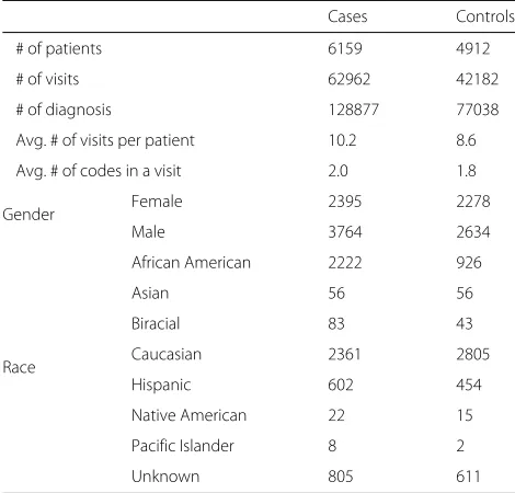
For the purpose of our analysis, we identified children with respiratory system-related symptoms by following the International Classification of Diseases (ICD-9) stan-dards. We extracted 323,555 children who had a diagnosis code of 786* (symptoms involving respiratory system and other chest symptoms, except 786.3: hemoptysis). After that, we filtered for those patients who had at least one encounter with one of these symptoms and more than two encounters before the age of 5, and were followed-up at least until the age of 8 years. Accordingly, the dataset size reduced significantly to 11,071 patients. The statistics and demographics of the study cohort are described in Table1. To demonstrate our interpretability approach on this data of pre-school children with respiratory system-related symptoms, we try to predict those children who will have asthma at school-age (cases) and those who will not have asthma at school-age (controls). Cases were defined as children who had at least one encounter with respiratory system-related symptoms before the age of 5, and at least one encounter with asthma diagnosis ICD
Table 1Basic statistics of the cohort
Cases Controls
# of patients 6159 4912
# of visits 62962 42182
# of diagnosis 128877 77038
Avg. # of visits per patient 10.2 8.6
Avg. # of codes in a visit 2.0 1.8
Gender Female 2395 2278
Male 3764 2634
Race
African American 2222 926
Asian 56 56
Biracial 83 43
Caucasian 2361 2805
Hispanic 602 454
Native American 22 15
Pacific Islander 8 2
Unknown 805 611
493* after the age of 6. Controls were defined as children who had at least one encounter with respiratory system-related symptoms before the age of 5, and no diagnosis of asthma for at least three years after school-age, which is age 6. This definition splits our data into 6159 cases and 4912 controls. It is worth mentioning here that, for this specific cohort, the proportion of cases is relatively high (56%), compared to other cohorts or diseases, in which the prevalence of the disease is usually less.
The LSTM and BiLSTM models require longitudinal patient-level data that has been collected over time across several clinical encounters. Therefore, we processed the dataset to be in the format of list of lists of lists. The outermost list corresponds to patients, the intermediate list corresponds to the time-ordered visit sequence each patient made, and the innermost list corresponds to the diagnosis codes that were documented within each visit. Only the order of the visits was considered and the times-tamp was not included.
Experimental setup
We implemented LSTM and BiLSTM models in PyTorch, and We also extended the implementation of Murdoch et al.[23] to decompose BiLSTM models. As the pri-mary objective of this paper is not predictive accuracy, we used standard best practices without much tuning to fit the models used to produce interpretations. All mod-els were optimized using Adam [27] with learning rate of 0.0005 using early stopping on the validation set. The total number of input features (diagnosis codes) was 930 for ICD-9 3-digits format and 3318 for ICD-9 4-digits format. Patients were randomly split into training (55%), valida-tion (15%), and test (30%) sets. The same proporvalida-tion of cases (56%) and controls (44%) was maintained among the training, validation, and test sets. Model accuracy is reported on the test set, and area under the curve (AUC) is used to measure the prediction accuracy, together with 95% confidence interval (CI) as a measure of variability.
Results
In this section, we first describe the models training results. After that, we provide quantitative evidence of the benefits of using CD interpretations and explore the extent to which it agrees with baseline interpretations. Finally, we present our qualitative analysis including an interactive visualization and demonstrate its utility for explaining predictive models using individual visit scores and relative contributions of subset of visits.
Models training
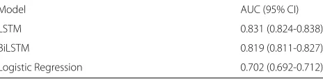
To validate the performance of the proposed interpretabil-ity approach, we train LSTM and BiLSTM models on the asthma dataset, which has two classes:c=1 for cases, andc=0 for controls. In addition, we compare the predic-tion performance of these models with a baseline logistic regression model. The average AUC scores for 10 runs, with random seeds, on the full test set are shown in Table2. Overall, the LSTM and BiLSTM models achieve higher AUC scores than baseline models such as logistic regression. Consequently, both models learned useful visit patterns for predicting school-age asthma.
Quantitative analysis
In this section, we conduct quantitative analysis to (1) val-idate the contextual decomposition of the trained models,
Table 2Average AUC of models trained on asthma dataset for the task of school-age asthma prediction
Model AUC (95% CI)
LSTM 0.831 (0.824-0.838)
BiLSTM 0.819 (0.811-0.827)
Logistic Regression 0.702 (0.692-0.712)
(2) evaluate the interpretations produced by the mod-els, and (3) understand the extent to which the learned patterns correlate with other baseline interpretations.
Validation of contextual decomposition for BiLSTMs
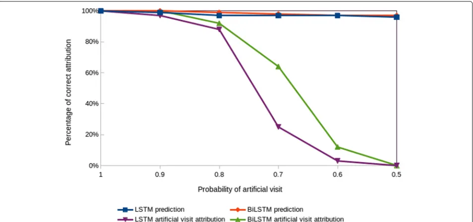
Objective:To verify that the contextual decomposition of LSTMs and BiLSTMs works correctly with our prediction task, we designed a controlled experiment in which we add the same artificial visit to each patient of certain class, testing whether the contextual decomposition will assign a high attribution score to the artificial visit with respect to that specific class.
Given a patientp and a corresponding binary labelc, we add an artificial visitvartwith one artificial diagnosis codedartto each patient’s visits listV. Thedart was cho-sen to be a synthetic diagnosis code which does not exist in the ICD-9 codes list. On the full datasetP, the artificial visit is added with probabilitypartto patients with label 1, and with probability 1−partto patients with label 0. As a result, whenpart= 1, all patients of class 1 will havevart, and consequently the model should predict label 1 with a 100% accuracy and contribution ofvartshould always be the maximum among other visits. Similarly, whenpart = 0.5, both classes will equally have patients withvart, and therefore vart does not provide any additional informa-tion about the label, and vart should thus have a small contribution.
Experimental settings:We train LSTM and BiLSTM models on the asthma dataset with the artificial visitvart setup. To measure the impact ofvart, we first addvartto patients of class c=1, with probability part, varying part from 1 to 0.5 with steps of 0.1. After that, we train both models on this modified dataset, and then calculate the contribution of each visit by using the CD algorithm. We run the experiment 5 times with a different random seed and report on the average correct attribution. The attribu-tion is correct if the highest contribuattribu-tion among all visits is assigned tovart.
Results:The results of our evaluation are depicted in Fig.1. Whenpart= 1, the models correctly attribute the prediction to the artificial visit at 100% accuracy. More-over, aspartbecomes smaller, the contribution of the arti-ficial visit goes down, sincevartbecomes less important. Finally, whenpart= 0.5, the contribution of the artificial visit becomes irrelevant and the model attributes the pre-diction to other visits. Both models LSTM and BiLSTM perform similarly with 100% and 0% attribution accu-racy atpart= 1 andpart=0.5, respectively. However, when
Fig. 1Validation of contextual decomposition for LSTM and BiLSTM for the classc=1. The attribution is correct if the highest contribution among all visits is assigned to the artificial visit. The prediction curves indicate the prediction accuracy for classc=1, which also represents the upper bound for the attribution accuracy
to unidirectional LSTM. Overall, we can conclude that whenever there is a clear visit-level pattern, the models learn that pattern and the contextual decomposition can appropriately attribute the prediction to the correct visit.
Evaluation of interpretations extracted from BiLSTMs
Before examining the visit-level dynamics produced by the CD algorithm, we first verify that it compares favor-ably to prior work for the standard use case of pro-ducing coefficients for individual visits, using logistic
regression. For longitudinal data such as EHR, a logistic regression model summarizes the EHR sequence ensem-ble to become aggregate features that ignore the tem-poral relationships among the feature elements. How-ever, when sufficiently accurate in terms of prediction, logistic regression coefficients are generally treated as a gold standard for interpretability. Additionally, when the coefficients are transformed by an exponential function, they can be interpreted as odds ratio [28]. In partic-ular, when applied to clinical outcomes prediction, the
Fig. 3CD scores for individual visits produced from LSTM and BiLSTM models trained for the task of predicting school-age asthma. Red is positive, white is neutral and blue is negative. The squares represent patient EHR time-ordered visits, and the label of each square indicates the visit number appended by the date of the visit. The upper row is the LSTM CD attributions and the lower row is the BiLSTM CD attributions
ordering of visits given by their coefficient value pro-vides qualitatively sensible measure of importance. There-fore, when validating the interpretations extracted using the CD algorithm we should expect to find a meaning-ful correlation between the CD scores and the logistic regression coefficients. To that end, we present our eval-uation of the interpretations extracted using the CD algo-rithm with respect to the coefficients produced by logistic regression.
Generating Ground Truth Attribution for Interpre-tation:Using our trained logistic regression model, we identified the most important three visits for each patient and used it as a baseline to evaluate the correlation between logistic regression coefficients and CD attribu-tions. First, we calculated the importance score for each diagnosis code. After that we used these scores to cal-culate the importance score for each visit, by summing the importance scores of the diagnosis codes included in each visit. The importance score for each diagnosis code is calculated as follows:
• extract statistically significant diagnosis codes, using p-value criterionp≤0.05
• for all significant diagnosis codes, calculate coefficients and odds ratios
• filter for diagnosis codes with odds ratio>1
• sort filtered diagnosis codes in descending order according to their odds ratios
• group the sorted diagnosis codes into 4 groups. Diagnosis codes with similar/closer odds ratios are grouped together
• assign an importance score for each group in descending order, based on the odds ratios of diagnosis codes in each group
Finally, we calculated the importance score for each visit, by summing the importance scores of the diagnosis codes occurred in that visit, and used the visits scores to identify the most important three visits for each patient. We run this analysis on a subset of 5000 patients, who have asthma, and for each patient the ground truth attri-bution baseline is the most important three visits, ordered according to their importance scores.
Evaluation: For each patient/ground-truth pair, we measured if the ground truth visits match the visit with the highest CD score for the same patient. We ranked the CD scores of visits for each patient and reported on the matching accuracy between the visit with the highest CD contribution and the three ground truth visits for each patient.
Results:The aggregated results for both LSTM and BiL-STM models are presented in Fig.2. Overall, we observe that, for the two models, the contextual decomposition attribution overlaps with our generated baseline ground truth attribution for at least 60% of the patient/ground-truth pairs. The matching between the top visit using the CD algorithm and the first top ground truth visit is 60%, the top two ground truth visits is 80%, the top three ground truth visits is 90%. These results confirm that there is a strong relationship between the importance scores generated using logistic regression coefficients and the CD importance scores based on the patterns an LSTM/BiLSTM model learns.
Qualitative analysis
After providing quantitative evidence of the benefits of CD to interpret the patient EHR visits importance, we now present our qualitative analysis using three types of experiments. First, we introduce our visualization and demonstrate its utility to interpret patient-specific pre-dictions. Second, we provide examples for using our CD-based algorithm to find the most predictive subset of visits. Finally, we show that the CD algorithm is capable of identifying the top scoring visit patterns and demonstrate this in the context of predicting school-age asthma.
Explaining predictions using individual visit scores
In this section, we present our interactive visualization and illustrate it with an example for both LSTM and BiL-STM models. The timeline in Fig.3represents a patient’s EHR time-ordered visits and the colors of the visits reflect the CD contributions of each visit to the predicted out-come. Moreover, hovering over the visits with the mouse will display the ICD codes documented by the clinician during the visit. Visualizing the CD contributions of each visit can be used to quickly explain why did the model make a certain prediction. For example, the patient shown in Fig.3was correctly predicted to have asthma at school age. He had 19 data points (visits) before the age of six years and it was all considered by the model. The
visualization indicated that visits 15 to 19 have the highest contribution to the prediction for both LSTM and BiL-STM models, and the ICD-9 codes included in these four visits are: 486 (pneumonia), 786 (symptoms involving res-piratory system and other chest symptoms), 493 (asthma), and 465 (acute upper respiratory infections of multiple or unspecified sites). Presenting such information to the clinician could be of a great help in the decision making process. For example, this specific patient has been fol-lowing up at the hospital from age 0 to 5 years, and he had respiratory-related complications throughout the 5 years. Typically, the physician will have to check the full his-tory of a patient to understand the patient condition and make a decision. In contrast, visualizing the CD scores for each visit as shown in Fig.3indicates that, for this specific patient, older visits are not very relevant. The visualiza-tion highlights that recent visits are more important to examine. This is probably due to the fact that continu-ing to have respiratory complications till age 5, just before school-age, is an important indication that this patient will likely continue to have asthma at school age.
Explaining predictions using relative contributions of subset of visits
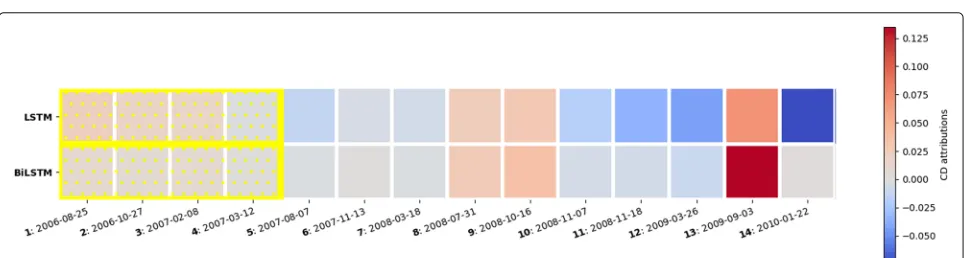
In this section, we first present our results for the imple-mentation of the algorithm introduced earlier for finding the most predictive subset of visits, and then we qualita-tively compare between the relative contributions of the subset of visits produced by LSTM and BiLSTM.
Figure4 shows an example of a patient who was cor-rectly predicted to have asthma at school-age. The patient made 14 visits between age 0 and 5 with different com-plications. The individual visit scores do not provide clear information about the critical time window which the physician needs to examine. However, using our algo-rithm for finding the most predictive subset of visits, the algorithm identified that grouping visits 1 to 4 together (highlighted in yellow) produced the maximum relative contribution to the predicted outcome, compared to other subset of visits. The ICD codes included in these visits
indicated that this patient has been diagnosed with con-genital anomalies as well as asthma before the age of 1, followed by organic sleep disorders and symptoms involv-ing respiratory system and chest in the followinvolv-ing years. Therefore, although the contributions of individual visits were not high, the relative contribution of grouping the visits together provided useful information to explain the prediction.
In general, we found that the relative contributions of subset of visits extracted from BiLSTM and LSTM are often similar. However, for some cases, such as the patient shown in Fig.5, we observed that contributions produced from BiLSMT are likely more clinically relevant than LSTM. This is possibly because BiLSTM mimics physi-cian practice by examining the EHR clinical visits not only in forward time order, but also considers the backward time order so that recent clinical visits are likely to receive higher importance.
Identifying top scoring patterns
We now demonstrate the utility of using the CD attri-butions to identify the top scoring patterns which was learned by the LSTM and BiLSTM models. To address this, we analysed for each patient for which the classc=1 (having asthma at school age) was correctly predicted, which visit patterns of length one and two visits had the highest positive contribution towards predicting that class. The results of this evaluation are summarized for one visit patterns in Table 3 and two visits patterns in Table 4. Overall, both models learn similar patterns for
both length one and two visits with no significant dif-ference. Moreover, the identified patterns are inline with the risk factors suggested in the literature for school-age asthma [29–31].
Discussion
In this study, we assessed the potential application of con-textual decomposition (CD) method to explain patient-specific risk predictions using quantitative and qualitative evaluation. Our results demonestrated that whenever a clear visit-level pattern exists, the LSTM and BiLSTM models learn that pattern and the contextual decompo-sition can appropriately attribute the prediction to the correct pattern. In addition, the results confirm that the CD score agrees to a large extent with the importance scores produced using logistic regression coefficients. Our main insight was that rather than interpreting the attribu-tion of individual patient visits to the predicted outcome, we could instead attribute a model’s prediction to a group of visits.
A potential limitation of our study is the identification of asthma patients using ICD codes. In particular, although using ICD codes to identify asthma is a popular practice in large-scale epidemiologic research, previous research showed that using ICD-9 codes have a moderate accu-racy of identifying children with asthma, compared to criteria-based medical record review [32]. In addition, the contextual decomposition approach was demonstrated on a single cohort of patients. Generalizing the findings and explanations of this study would require assessing
Table 3Top scoring patterns of length 1 visit, produced by the contextual decomposition of LSTM and BiLSTM models on the asthma data
LSTM BiLSTM
ICD Codes Frequency% ICD Codes Frequency%
1 493.9 Asthma Unspecified 40% 493.9 Asthma Unspecified 34%
2 493.9,786.0 Asthma Unspecified, Dyspnea and Respiratory Abnormalities
13% 786.2 Cough 15%
3 786.0 Dyspnea and Respiratory Abnormalities 11% 493.9,786.0 Asthma Unspecified, Dyspnea and Respiratory
21%
4 493.9,786.2 Asthma Unspecified,Cough 10% 786.0 Dyspnea and Respiratory Abnormalities 10%
5 465.9,493.9 Acute Upper Respiratory Infections of Unspecified Site, Asthma Unspecified
9% 493.9,786.2 Asthma Unspecified, Cough 9%
6 493.0 Extrinsic Asthma 4% 465.9,493.9 Acute Upper Respiratory Infections of
Unspecified Site,Asthma Unspecified 8%
7 486,493.9 Pneumonia, Asthma Unspecified 4% 465.9,786.2 Acute Upper Respiratory Infections of Unspecified Site,Cough
5%
8 465.9,493.9,786.2 Acute Upper Respiratory Infec-tions of Unspecified Site, Asthma Unspecified, Cough
3% 486,493.9 Pneumonia, Asthma Unspecified 3%
9 382.9,493.9 Unspecified Otitis Media, Asthma Unspecified
3% 486,493.9 Pneumonia, Asthma Unspecified 3%
Table 4Top scoring patterns of length 2 visit, produced by the contextual decomposition of LSTM and BiLSTM models on the asthma data
LSTM BiLSTM
ICD Codes Frequency% ICD Codes Frequency%
1 [493.9],[493.9] [Asthma Unspecified],[Asthma Unspecified] 13% [493.9], [493.9] [Asthma Unspecified],[Asthma Unspeci-fied]
11%
2 [493.9,786.0],[493.9][Asthma Unspecified, Dyspnea and Respiratory Ab-normalities], [Asthma Unspecified]
2% [493.9,786.0],[493.9][Asthma
Unspecified, Dyspnea and Res-piratory Ab-normalities], [Asthma Unspecified]
2%
3 [493.9],[493.9,786.0] [Asthma Unspecified], [Asthma Unspecified, Dysp-nea and Respiratory Abnormalities]
2% [493.9],[493.9,786.0][Asthma
Unspecified], [Asthma Unspecified, Dysp-nea and Respiratory Abnormalities]
2%
4 [493.9], [V20.2] [Asthma Unspecified], [Routine Infant or Child Health Check]
2% [493.9], [V20.2][Asthma
Unspecified], [Routine Infant or Child Health Check]
2%
5 [493.9,786.2], [493.9] [Asthma Unspecified, Cough], [Asthma Unspecified]
2% [493.9,786.2], [493.9][Asthma
Unspecified, Cough], [Asthma Unspecified]
1%
multiple datasets represeting multiple cohorts, diseases, and age groups.
Conclusion
In this paper, we have proposed using contextual decom-position (CD) to produce importance scores for individual visits and relative importance scores for a group of vis-its, to explain decisions of risk prediction models. In addition, we developed an interactive visualization tool and demonstrated, using a concrete case study with real EHR data, how CD scores offer an intuitive visit-level interpretation. This movement beyond single visit impor-tance is critical for understanding a model as complex and highly non-linear as BiLSTM. The potential exten-sion of our approach to other sources of big medical data (e.g. genomics and imaging), could generate valuable insights to assist decision-making for improved diagnosis and treatment.
Consent to publish Not applicable.
Abbreviations
AUC: Area under the curve; BiLSTM: Bidirectional long short-term memory network; CD: Contextual decomposition; DNN: Deep neural network; EHR: Electronic health record; ICD: International Classification of Diseases; LSTM: Long short-term memory network; RNN: Recurrent neural network
Acknowledgements
We would like to thank Zien Ali for her technical help with the experimental analysis.
Authors’ contributions
RA developed the idea, implemented the method, conducted the
experiments, and drafted the manuscript. SB and QM supervised every step of the work and provided critical review and valuable input. IJ contributed to the clinical use case selection and cohort design. All authors read and approved the final manuscript.
Funding
This work is supported in part by Sidra Medicine under grant (SDR200043). The funder had no role in study design, data collection and analysis, decision to publish, or preparation of the manuscript.
Availability of data and materials
The data that support the findings of this study are available from Cerner HealthFacts but restrictions apply to the availability of these data, which were used under license for the current study, and so are not publicly available. Data however can be directly requested from Cerner HealthFacts on reasonable request.
Ethics approval and consent to participate
This research was approved by the Institutional Review Board at Sidra Medicine (protocol number 1804023464). Informed consent was exempted because of the retrospective nature of this research. Patient data were anonymized and de-identified by the data provider.
Competing interests
The authors declare that they have no competing interests.
Author details
1Machine Learning Group, Sidra Medicine, Doha, Qatar.2Department of
Computer Science and Engineering, Qatar University, Doha, Qatar.3Division of Pediatric Pulmonology, Sidra Medicine, Doha, Qatar.
Received: 28 March 2019 Accepted: 28 October 2019
References
1. Xiao C, Choi E, Sun J. Opportunities and challenges in developing deep learning models using electronic health records data: A systematic review. J Am Med Assoc. 2018;25(10):1419–28.http://doi.org/10.1093/ jamia/ocy068.
2. Golas SB, Shibahara T, Agboola S, et al. A machine learning model to predict the risk of 30-day readmissions in patients with heart failure: A retrospective analysis of electronic medical records data. BMC Med Inform Decis Making. 2018;18(44):1–17. https://doi.org/10.1186/s12911-018-0620-z.
4. Shickel B, Tighe PJ, Bihorac A, Rashidi P, J Biomed Health Inform IEEE. Deep EHR: A Survey of Recent Advances in Deep Learning Techniques for Electronic Health Record (EHR) Analysis. 20171–14.https://doi.org/10. 1109/JBHI.2017.2767063.
5. Adkins DE. Machine Learning and Electronic Health Records: A Paradigm Shift. Am J Psychiatr. 2017;174(2):93–4.https://doi.org/10.1176/appi.ajp. 2016.16101169.
6. Lipton ZC, Kale DC, Elkan C, Wetzel R. Learning to Diagnose with LSTM Recurrent Neural Networks. 20151–18.https://doi.org/10.14722/ndss. 2015.23268.
7. Esteban C, Staeck O, Yang Y, Tresp V. Predicting Clinical Events by Combining Static and Dynamic Information Using Recurrent Neural Networks. In: 2016 IEEE International Conference on Healthcare Informatics (ICHI); 2016.https://doi.org/10.1109/ichi.2016.16. 8. Pham T, Tran T, Phung D, Venkatesh S. DeepCare : A Deep Dynamic
Memory Model for Predictive Medicine. 2017;i:1–27.http://arxiv.org/abs/ arXiv:1602.00357v2.
9. Jagannatha AN, Yu H. Bidirectional RNN for Medical Event Detection in Electronic Health Records. Association for Computational Linguistics; 2016.https://doi.org/10.18653/v1/n16-1056.
10. Liu J, Zhang Z, Razavian N. Deep EHR: Chronic Disease Prediction Using Medical Notes. In: Proceedings of the 3rd Machine Learning for Healthcare Conference. PMLR 85; 2018. p. 440–464.http://arxiv.org/abs/ arXiv:1808.04928v1.
11. Wunnava S, Qin X, Kakar T, Sen C, Rundensteiner EA, Kong X. Adverse Drug Event Detection from Electronic Health Records Using Hierarchical Recurrent Neural Networks with Dual-Level Embedding. Drug Safety. 2019;42(1):113–22.https://doi.org/10.1007/s40264-018-0765-9. 12. Ahmad MA, Eckert C, Teredesai A. Interpretable Machine Learning in
Healthcare. In: Proceedings of the 2018 ACM International Conference on Bioinformatics, Computational Biology, and Health Informatics - BCB ’18; 2018. p. 559–560.https://doi.org/10.1145/3233547.3233667.
13. Murdoch WJ, Singh C, Kumbier K, Abbasi-Asl R, Yu B. Interpretable machine learning: definitions, methods, and applications. 20191–11. http://arxiv.org/abs/1901.04592.
14. Baumel T, Nassour-Kassis J, Cohen R, Elhadad M, Elhadad N. Multi-Label Classification of Patient Notes a Case Study on ICD Code Assignment. 2017.http://arxiv.org/abs/1709.09587.
15. Ma F, Chitta R, Zhou J, You Q, Sun T, Gao J. Dipole: Diagnosis Prediction in Healthcare via Attention-based Bidirectional Recurrent Neural Networks. 2017.https://doi.org/10.1145/3097983.3098088.
16. Choi E, Bahadori MT, Song L, Stewart WF, Sun J. GRAM: Graph-based Attention Model for Healthcare Representation Learning. 20161–15. https://doi.org/10.1145/3097983.3098126.
17. Choi E, Bahadori MT, Kulas JA, Schuetz A, Stewart WF, Sun J. RETAIN: An Interpretable Predictive Model for Healthcare using Reverse Time Attention Mechanism (NIPS). 2016.http://arxiv.org/abs/1608.05745. 18. Choo J, Kwon BC, Choi E, Kim YB, Kim JT, Choi M-J, Kwon S, Sun J.
RetainVis: Visual Analytics with Interpretable and Interactive Recurrent Neural Networks on Electronic Medical Records. IEEE Trans Vis Comput Graph. 2018;25(1):299–309.https://doi.org/10.1109/tvcg.2018.2865027. 19. Zhang J, Kowsari K, Harrison JH, Lobo JM, Barnes LE. Patient2Vec: A
Personalized Interpretable Deep Representation of the Longitudinal Electronic Health Record. IEEE Access. 2018;6:65333–46.https://doi.org/ 10.1109/ACCESS.2018.2875677.
20. Xu Y, Biswal S, Deshpande SR, Maher KO, Sun J. RAIM: Recurrent Attentive and Intensive Model of Multimodal Patient Monitoring Data. 2018.https://doi.org/10.1145/3219819.3220051.
21. Che Z, Purushotham S, Khemani R, Liu Y. Distilling Knowledge from Deep Networks with Applications to Healthcare Domain. 2015.http:// arxiv.org/abs/1512.03542.
22. Che Z, Purushotham S, Khemani R, Liu Y. Interpretable Deep Models for ICU Outcome Prediction,. AMIA Annu Symp Proc AMIA Symp. 2016;2016: 371–80.
23. Murdoch WJ, Liu PJ, Yu B. Beyond word importance: Contextual decomposition to extract interactions from lstms. arXiv preprint arXiv:1801.05453. 2018.
24. Hochreiter S, Schmidhuber J. Long short-term memory. Neural Comput. 1997;9(8):1735–80.https://doi.org/10.1162/neco.1997.9.8.1735. 25. Schuster M, Paliwal KK. Bidirectional recurrent neural networks. IEEE Trans
Sig Process. 1997;45(11):2673–81.https://doi.org/10.1109/78.650093.
26. DeShazo JP, Hoffman MA. A comparison of a multistate inpatient EHR database to the HCUP nationwide inpatient sample. BMC Health Serv Res. 2015;15(1):.https://doi.org/10.1186/s12913-015-1025-7.
27. Kingma DP, Ba J. Adam: A method for stochastic optimization. 2014. http://arxiv.org/abs/1412.6980.
28. Szumilas M. Explaining odds ratios,. J Can Acad Child Adolesc Psychiatry. 2010;19(3):227–9.
29. Morais-Almeida M, Gaspar A, Pires G, Prates S, Rosado-Pinto J. Risk factors for asthma symptoms at school age: an 8-year prospective study,. Allergy Asthma Proc. 2007;28(2):183–9.
30. Bjerg A, Rönmark E. Asthma in school age: prevalence and risk factors by time and by age. The Clinical Respiratory Journal. 2008;2:123–6.https:// doi.org/10.1111/j.1752-699X.2008.00095.x.
31. Szentpetery SS, Gruzieva O, Forno E, Han Y-Y, Bergström A, Kull I, Acosta-Pérez E, Colón-Semidey A, Alvarez M, Canino GJ, Melén E, Celedón JC. Combined effects of multiple risk factors on asthma in school-aged children,. Respir Med. 2017;133:16–21.https://doi.org/10. 1016/j.rmed.2017.11.002.
32. Juhn Y, Kung A, Voigt R, Johnson S. Characterisation of children’s asthma status by ICD-9 code and criteria-based medical record review. Prim Care Respir J. 2010;20(1):79–83.https://doi.org/10.4104/pcrj.2010.00076.
Publisher’s Note