https://doi.org/10.5194/amt-10-3345-2017 © Author(s) 2017. This work is distributed under the Creative Commons Attribution 3.0 License.
Application of Gauss’s theorem to quantify localized surface
emissions from airborne measurements of wind and trace gases
Stephen Conley1,6, Ian Faloona1, Shobhit Mehrotra1, Maxime Suard1, Donald H. Lenschow2, Colm Sweeney4, Scott Herndon3, Stefan Schwietzke4,5, Gabrielle Pétron4,5, Justin Pifer6, Eric A. Kort7, and Russell Schnell5 1Department of Land, Air, & Water Resources, University of California, Davis, CA 95616, USA
2Mesoscale and Microscale Meteorology Laboratory, National Center for Atmospheric Research, Boulder, CO 80307, USA
3Aerodyne Research, Inc, Billerica, MA 01821, USA
4Cooperative Institute for Research in Environmental Sciences, University of Colorado, Boulder, CO 80305, USA 5NOAA Earth System Research Laboratory, Boulder, CO, USA
6Scientific Aviation, Inc., Boulder, CO, USA
7Climate and Space Sciences and Engineering, University of Michigan, Ann Arbor, MI, USA
Correspondence to:Stephen Conley ([email protected], [email protected]) Received: 24 February 2017 – Discussion started: 18 April 2017
Revised: 11 August 2017 – Accepted: 16 August 2017 – Published: 13 September 2017
Abstract. Airborne estimates of greenhouse gas emissions are becoming more prevalent with the advent of rapid com-mercial development of trace gas instrumentation featuring increased measurement accuracy, precision, and frequency, and the swelling interest in the verification of current emis-sion inventories. Multiple airborne studies have indicated that emission inventories may underestimate some hydrocar-bon emission sources in US oil- and gas-producing basins. Consequently, a proper assessment of the accuracy of these airborne methods is crucial to interpreting the meaning of such discrepancies. We present a new method of sampling surface sources of any trace gas for which fast and pre-cise measurements can be made and apply it to methane, ethane, and carbon dioxide on spatial scales of ∼1000 m, where consecutive loops are flown around a targeted source region at multiple altitudes. Using Reynolds decomposition for the scalar concentrations, along with Gauss’s theorem, we show that the method accurately accounts for the smaller-scale turbulent dispersion of the local plume, which is of-ten ignored in other average ”mass balance” methods. With the help of large eddy simulations (LES) we further show how the circling radius can be optimized for the microme-teorological conditions encountered during any flight. Fur-thermore, by sampling controlled releases of methane and ethane on the ground we can ascertain that the accuracy of
the method, in appropriate meteorological conditions, is of-ten better than 10 %, with limits of detection below 5 kg h−1 for both methane and ethane. Because of the FAA-mandated minimum flight safe altitude of 150 m, placement of the air-craft is critical to preventing a large portion of the emission plume from flowing underneath the lowest aircraft sampling altitude, which is generally the leading source of uncertainty in these measurements. Finally, we show how the accuracy of the method is strongly dependent on the number of sampling loops and/or time spent sampling the source plume.
1 Introduction
“bottom-up” inventories are developed by aggregating statistical cor-relates of individual process emissions to such mapping vari-ables as population density, energy consumption, head of cat-tle, etc., extrapolating to total emissions using a relatively small number of direct measurements. On the other hand, at-mospheric scientists have long striven to use measurements from global surface networks, aircraft campaigns, and satel-lites to try to determine emissions based on the amounts and build-up rates of observed trace gases. Aircraft and satellites, the “top-down” approach, conveniently integrates the multi-tude of sources, but is heavily reliant on a detailed knowl-edge of atmospheric transport. Top-down methods also suf-fer from difficulties attributing sources and generalizing mea-surements made over a relatively short time period. Attempts to reconcile these two distinct methods on global (Muhle et al., 2010) and continental scales (Gerbig et al., 2003; Miller et al., 2013) have often indicated an apparent underestima-tion by the bottom-up methods of a factor 1.5 or more.
In principle, the aircraft top-down measurements can be conducted at all the atmospheric scales to better understand and identify the emissions at comparable scales. For long-lived greenhouse gases, which readily disperse throughout the atmosphere, the global scale is very instructive. The seminal experiment began with Keeling’s acclaimed CO2 curve (1960), and has continued through more contemporary techniques by Hirsch et al. (2006) and Neef et al. (2010) for CH4and N2O, respectively. At progressively smaller scales more details of the source strengths and apportionment can be made: from synoptic or continental scales which can help constrain national inventories (Bergamaschi et al., 2005) or specific biogeographic regions (Gallagher et al., 1994), to mesoscale investigations that estimate emissions from urban areas (Mays et al., 2009; Turnbull et al., 2011; Wecht et al., 2014) or specific oil- and gas-producing fields (Karion et al., 2013; Petron et al., 2014) and even down to individual point/area sources on the order of 10–100 m size (Denmead et al., 1998; Lavoie et al., 2015; Roscioli et al., 2015).
Aircraft in situ measurements are particularly useful for top-down methods at the sub-mesoscale because they can be used to measure the air both upwind and downwind of a source region. However, deployments tend to be costly and thus sporadic. As far as we know, the aircraft methods used so far can be categorized into three types. First, there is the eddy covariance technique that is carried out at low altitudes wherein the vertical fluxes of gases carried by the turbulent wind are measured by tracking rapid fluctuations of both con-centrations and vertical wind (Hiller et al., 2014; Ritter et al., 1994; Yuan et al., 2015). This method is generally thought to be the most direct, but it is limited to small footprint re-gions which must be repeatedly sampled for sufficient statis-tical confidence, requires a sophisticated verstatis-tical wind mea-surement, and can be subject to errors due to flux divergence between the surface and the lowest flight altitude and accel-eration sensitivity of the gas sensor. The second and by far the most common approach is what chemists usually refer to
as “mass balance” and what is known in the turbulence com-munity as a “scalar budget” technique. Many different sets of assumptions and sampling strategies are employed, but the overall goal is to sample the main dispersion routes of the surface emissions as they make their way into the overly-ing atmosphere after first accumulatoverly-ing near the surface. The scales that can be addressed by this method are from a few kilometers (Alfieri et al., 2010; Hacker et al., 2016; Hiller et al., 2014; Tratt et al., 2014) to tens of kilometers (Caulton et al., 2014; Karion et al., 2013; Wratt et al., 2001) to even po-tentially hundreds of kilometers (Beswick et al., 1998; Chang et al., 2014), and this approach has been the focus of recent measurements in natural gas production basins. These basins present a source apportionment challenge in that emissions from multiple sources (agriculture, oil and gas wells, geo-logic seepage, etc.) commingle as the air mass travels across the basin. The third method of source quantification is to ref-erence measurements of the unknown trace gas to a refref-erence trace gas with a metered release (tracer) or otherwise-known emission rate and assume that the tracer and the scalar of in-terest have the same diffusion characteristics. Typically this tracer release technique is applied to small scales of tens to hundreds of meters (Czepiel et al., 1996; Lamb et al., 1995; Roscioli et al., 2015), but the principle has been attempted at the basin (Peischl et al., 2013) and continental (Miller et al., 2012) scales using a reference trace gas with a suitable known emission rate such as CO2or CO.
The airborne mass balance flight strategies can be grouped into three basic patterns: a single height transect around a source assuming a vertically uniformly mixed boundary layer (Karion et al., 2013), single height upwind/downwind (Wratt et al., 2001) or sometimes just downwind flight legs (Con-ley et al., 2016; Hacker et al., 2016; Ryerson et al., 1998), multiple flight legs at different altitudes (Alfieri et al., 2010; Gordon et al., 2015; Kalthoff et al., 2002), or just a “screen” on the downwind face of the box (Karion et al., 2015; Lavoie et al., 2015; Mays et al., 2009).
In this study we first present the general analytical method used to derive emission estimates using airborne measure-ments. Next, we investigate the structure of a generalized dispersing plume using large eddy simulation (LES) to better understand the optimal sampling strategies for quantifying near-surface gas sources. Because the wind fields of turbu-lent flows cannot be predicted in detail, we do not attempt to compare specific features of our observations with specific LES results, but rather we use the numerical experiments to guide the development of the observational methodology. For example, by investigating the LES flux divergence profiles in the layer below the lowest flight altitude, we are able to es-timate the contribution of this unmeasured component to the overall source strength. We then evaluate the accuracy of the approach using coordinated planned release experiments and by applying the method to CO2emitted from several power plant plumes to compare with reported emissions.
2 Data collection
2.1 Airborne instrumentation
The airborne detection system is flown on a fixed wing single-engine Mooney aircraft, extensively modified for re-search as described in Conley et al. (2014). Ambient air is collected through∼5 m of tubing (Kynar, Teflon, and stain-less steel) that protrudes out of backward-facing aluminum inlets mounted below the right wing. In situ CH4, CO2, and water vapor are measured with a Picarro 2301f cavity ring down spectrometer as described by Crosson (2008), which is operated in its precision mode at 1 Hz. In situ ethane (C2H6) is measured with an Aerodyne methane/ethane tunable diode infrared laser direct absorption spectrometer (Yacovitch et al., 2014). There is a 5–10 s time lag in both analyzers that depends on the flow rate and tubing diameter. We use a 1/8 in. OD (3.175 mm) stainless line for the Picarro (∼0.2 slpm flow rate), and a 6.3 mm (1/4 in.) Teflon line for the CH4/C2H6 spectrometer (∼4 slpm flow rate). This results in lag times of∼5 s for the Aerodyne and∼10 s for the Picarro. The lag time for the Picarro is calculated using a “breath test”, whereby we exhale into the air inlet and mea-sure the time required for the CO2measurement to peak. The ethane lag time is adjusted to maximize the correlation be-tween the ethane and Picarro methane time series in plumes where both gases are emitted. Both lag times are slightly de-pendent on pressure, i.e., with a typical altitude change of ∼1 km, the change in lag time is less than 10 %, and is in-consequential when applying this method within a few hun-dred meters from the surface. The horizontal wind speed and direction, sampled at 1 Hz, is based on a standard aircraft pitot-static pressure airspeed measurement and a dual GPS compass that determines aircraft heading and ground speed. The accuracy of the horizontal wind measurement is about 0.2 m s−1 (Conley et al., 2014). The horizontal wind is
cal-ibrated periodically by flying ∼5 km L-shaped patterns in the free troposphere; a heading rotation and airspeed adjust-ment is made to the wind calculation to minimize the de-pendence of the wind on aircraft heading. These adjustments typically amount to less than 2◦rotation and 3 % adjustment of the airspeed. In flying the tight circle patterns described below, the pilot does not adjust the rudder trim to use the same calibration coefficients in the wind measurement cal-culation throughout the flight.
2.2 Large eddy simulations
In order to study the plume behavior of surface emissions as it relates to sampling in the stacked circles, we use the LES module of WRF V3.6.1. WRF-LES explicitly resolves the largest turbulent eddies by filtering the Navier–Stokes scalar conservation equations at some scale in the inertial subrange, and allowing the smaller motions beyond the cut-off to be modeled using a sub-grid (also called a sub-filter) scale turbulence parameterization that is based on properties of the larger-scale, resolved flow. Because the aircraft data is typically sampled at 1 Hz and the true airspeed is around 70 m s−1, we use an LES horizontal grid size roughly half (40 and 50 m) the distance between aircraft data samples. Because periodic lateral boundary conditions are imposed on the WRF-LES variables, care must be taken to ensure that the effluent does not reach the lateral boundaries of the simulation domain. On the other hand, WRF-LES does not allow for parallelized computation, making the simulations quite expensive in terms of computation time. We therefore struck a balance between a large enough domain in hori-zontal extent (6 and 8 km) such that the effluent would not reach the downwind boundary before the end of our sim-ulation, while maintaining a grid size small enough to re-solve scales of the aircraft observations. The vertical domain needs to be large enough to encompass a developing convec-tive boundary layer (CBL), while at the same time containing substantial free tropospheric flow above to serve as a reser-voir that can feed momentum and free-tropospheric scalars to the CBL. Moreover, the stable region (potential temper-ature lapse rate dθ/dz=5 C km−1) between the CBL inver-sion base and the top of the domain had to be large enough to damp any wave activity before it could reflect off the up-per boundary and create spurious motions throughout the do-main.
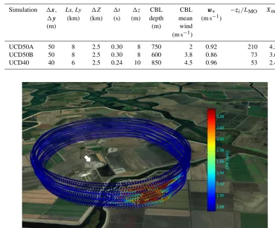
ki-Table 1.Domain and micrometeorological parameters for the three WRF-LES experiments in this study.Lrepresents the Monin–Obukhov length.
Simulation 1x, Lx, Ly 1Z 1t 1z CBL CBL w∗ −zi/LMO Xmax
1y (km) (km) (s) (m) depth mean (m s−1)
(m) (m) wind
(m s−1)
UCD50A 50 8 2.5 0.30 8 750 2 0.92 210 4.5
UCD50B 50 8 2.5 0.30 8 600 3.8 0.86 73 3.6
UCD40 40 6 2.5 0.24 10 850 4.5 0.96 53 2.4
Figure 1.Map of the airplane flight pattern sampling a methane plume emanating from an underground storage facility. Wind direction is indicated by the white arrow and the methane mixing ratio is given by the color bar to the right. This flight was conducted on 28 June 2016 and took place between 12:46 and 13:52 LT at altitudes ranging from 91 to 560 m with a loop diameter of approximately 3 km. The measured methane emission rate was 763±127 kg h−1.
netic energy. The conditions for the three simulations are listed in Table 1, and based on the different wind speeds they range from moderate to strongly convective boundary layers (-zi/LMO from ∼50 to ∼200, where LMO is the Monin– Obukhov length andzi is the CBL depth.)
3 Methods
3.1 Theory of measurement using Gauss’s theorem We use an integrated form of the scalar budget equation for a passive, conservative scalar in a turbulent fluid to es-timate the emission of a gas of interest within a cylindri-cal volume V. The volume is circumscribed by a series of closed aircraft flight paths (typically circular) flown around the emission source over a range of altitudes. The alti-tudes encompass the lowest safe flight level (usually 75– 150 m a.g.l.) up to an altitude where no discernable change
in the trace gas mixing ratio,χ, is observed around the flight loop,zmax. The scalar in our case is the mass concentration (i.e., density of a chemically unreactive species in a turbulent flow field,u=ui+vj+wk; its Reynolds decomposition is
c=C+c0, whereC is the mean concentration around each loop andc0 is the departure from the loop mean. Figure 1 shows an actual example of the effluent sampled by the air-craft in a sequence of stacked pathsl that circumscribe an area,A, enclosing the source in a volume,V. The effluent is carried downwind as it mixes upward in the CBL. A virtual surface circumscribed by the circular flight tracks is assumed enclosing the source and extending above the vertical extent of the plume so that there is no vertical transport above that level. To estimate the source strength, we start with the inte-gral form of the continuity equation:
Qc=
∂m
∂t
+
Z Z Z
whereh idenotes an average over the volumeV,Qc is the sum of the internal sources and sinks ofcwithinV, andmis the total mass ofc within the volumeV. At this point, we recognize that the flux divergence is composed of two terms
∇ ·cu=u· ∇c+c∇ ·u. (2)
In Sect. 3.2 we perform a scale analysis of the terms on the right-hand side (rhs) of Eq. (2) and show that the sec-ond term, which is proportional to the horizontal wind diver-gence, may be neglected under our normal flight protocol. This is fortunate because of the difficulty in accurately es-timating the horizontal wind divergence from aircraft mea-surements (Lenschow et al., 2007). The vertical flux across the top of the flight cylinder is assumed to be zero, and the flux from the bottom (ground) is the surface source we are measuring. This leaves us with only the horizontal flux, i.e., cuh, where uh (=ui+vj). In order to minimize the contribution from the horizontal wind divergence term, we remove the loop mean concentration,C, which does not al-ter the first al-term on the rhs because∇C=0, so that Eq. (2) becomes
uh· ∇c+c∇ ·uh=uh· ∇(c0). (3) Next, we use Gauss’s theorem to relate the volume integral to a surface integral around the volume that is sampled by the aircraft flight loops:
Qc=
∂m
∂t
+
Z Z Z
∇ ·(c0u)dV =
∂m
∂t
+
Z I
c0u· ˆndS, (4) whereSis the surface enclosingV andnˆis an outward point-ing unit vector normal to the surface.
The surface integral can be broken into three elements: a cylinder extending from the ground up to a level above significant modification by the emission, the ground surface circumscribed by a low-level (virtual) circular flight path (z=0), and a nominally horizontal surface circumscribed by a flight path above the level modified by the source (z=zmax). We assume there is no significant flux (other than the source of interest) into or out of the ground. Next, the surface integral is estimated solely from a sequence of closed path integrals measured by the aircraft at multiple flight lev-els to estimate the right side of Eq. (5) (blue dashed lines in Fig. 1),
Z I
c0u· ˆndS= zmax
Z
0
I
c0uh· ˆndldz, (5)
wherelis the flight path.
Combining Eqs. (4) and (5) leads to the result that is the basis for this measurement technique where a series of hor-izontal loops at different altitudes are flown around a source region:
Qc=
∂m ∂t
+ zmax
Z
0
I
c0uh· ˆndldz. (6)
Along each path the instantaneous outward flux is computed and summed over the loop to yield the mean flux divergence via Gauss’s theorem. A temporal trend of the total mass within the volume (∂m∂t) can be estimated from the flight data and added to the flux divergence integral to obtain the emis-sion rate.
3.2 Divergence uncertainty
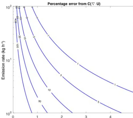
In order to estimate the relative error in the horizontal diver-gence term that we are eliminating, we perform a scale analy-sis of the relative size of the two terms in Eq. (2), using some typical values of the CBL parameters (convective velocity scalew∗=1 m s−1, boundary layer depth,zi=1000 m), and sampling geometry (flying at a radius of 1 km around a point source.) The Taylor (1922) statistical theory of dispersion in a homogenous and stationary turbulent fluid predicts that the root mean square lateral (σy) and vertical (σz) dispersion pa-rameters increase linearly with time, or equivalently advec-tion distance, downwind in the near field. Weil (1988) shows several examples of the growth of both of these parameters downwind to be∼0.5w∗, which we use here for a rough es-timate of a conical plume spreading to quantify the dilution of the source’s emission as it travels downwind to be inter-cepted by the aircraft. We use a large background mixing ratio characteristic of global CH4(∼1.9 ppmv), estimate the mean gradient by the plume concentration divided by the dis-tance downwind, and assume a conservatively large horizon-tal wind divergence of 10−5s−1, which may in fact be typical for our small sampling region (Stull, 1988). The results are shown in Fig. 2 and, for all but the smallest sources of a few kilograms per hour and wind speeds below 1 m s−1, the di-vergence term is at least an order of magnitude smaller than the gradient term.
3.3 Applying the theory to the LES results
We calculated a comparable estimate ofQcin the LES do-main from the air density, concentration, and wind along circular flight paths as a virtual aircraft would fly. Willis and Deardorff (1976) generalized results of their convection tank experiments to downwind dispersion in the convective boundary layer (CBL) in terms of a dimensionless length scaleX, the ratio of the horizontal advection time to the large eddy turnover time:
X=xw∗
U zi
, (7)
Figure 2.Graphical representation of the relative magnitude (%) of the contribution of the horizontal wind divergence to the hori-zontal advective terms in Eq. (3), as a function of wind speed and source magnitude for methane, using a typical global background of 1.9 ppm and divergence of 10−5s−1.
Figure 3 shows the crosswind-integrated concentration profile for the plume release in the UCD50B WRF-LES run as function ofX, and normalized height,Z=z/zi. Because of the time limitation due to the periodic boundary condi-tions, the plume is averaged for only ∼15 min of simula-tion time which is just under a large eddy turnover time for the conditions of the run. The results displayed in Fig. 3 are in good qualitative agreement with the results of Willis and Deardorff (1976) and Weil et al. (2012), save for the release being at the surface in our LES study, and at Z=0.067 for the above studies (see Figs. 1 and 2 of Weil et al., 2012). Fig-ure 3 shows the maximum concentration being lofted near
X∼0.2 and leveling off nearZ∼0.8 aroundX∼0.6; be-yondX >1.5 the plume is fairly well mixed throughout the extent of the boundary layer.
3.4 The upwind-directed turbulent flux
Horizontal turbulent fluxes are generally ignored in boundary layer budget studies due to the fact that while they are often sizeable in magnitude they do not change significantly over horizontal length scales under consideration (the horizontal homogeneity assumption). In the vicinity of a point source, however, this is not likely. The method outlined here esti-mates source emissions using a measured horizontal flux that incorporates wind and scalar measurements at 1 Hz sample rate, resolving scales of∼70 m (Conley et al., 2014), which should include nearly all of the turbulent contributions to the horizontal flux. Here we consider the nature of this turbu-lent flux and the error in emission estimates if only the mean
Figure 3.Relative cross wind integrated concentrations of an efflu-ent plume released at the surface in the UCD50B simulation. The data are averaged over 15 min of simulation time and normalized by the maximum concentration.
transport were considered. We start with the budget equa-tion for a horizontal scalar flux in a horizontally homoge-neous turbulent flow where the molecular diffusive/viscous term has been neglected (Wyngaard, 2010),
dc0u0 dt = −u
02∂C
∂x −u
0w0∂C
∂z −c
0w0∂U
∂z − ∂c0u02
∂x
−∂c 0u0w0
∂z −
1
ρc
0∂p 0
∂x, (8)
whereρis density andp0is the pressure fluctuation. We then assume stationarity and integrate across the source from a point just upwind to a point within the plume and obtain
x
Z
0−
∂c0u0
∂x0 dx 0= −1
U
x
Z
0−
u02 ∂C ∂x+0+u
0w0∂C
∂z +c
0w0∂U
∂z
+∂c 0u02
∂x0 +
∂c0u0w0
∂z +
1
ρc
0∂p 0
∂x0
#
dx0. (9)
We further assume that although the scalar field is not ho-mogeneous the flow field is, and the background horizontal
c-flux upwind is much smaller than the flux induced by the point source. This results in an equation for the in-plume flux
c0u0= − 1
U
u02 Cx−Cbckg+u0w0 x
Z
0−
∂C ∂zdx
0+ x
Z
0−
c0w0
∂U ∂z +
x
Z
0−
∂c0u02
∂x0 +
∂c0u0w0
∂z +
1
ρc
0∂p 0
∂x0
!
dx0
.
The first three terms on the rhs of Eq. (10) are negative within the plume with their largest magnitudes on the upwind side and diminishing downwind. On the largest, boundary-layer-filling eddy scales, the mean concentration ofC down-wind of a source is greater than in the updown-wind region, (Cx−Cbckg)>0, and therefore the first term is negative, but decreases in magnitude with distance downwind. How-ever, this term is also positive on smaller scales within the plume where the mean gradient is directed upwind towards the source, and is most likely responsible for the specious intuitive impression that the horizontal turbulent flux should transport the plume downwind from the source along with the mean wind advection. Moreover, the second and third terms on the rhs are negative because the momentum flux,u0w0, and mean vertical gradient,∂C/∂z, are negative while the verti-cal turbulent flux,c0w0, and wind shear,∂U/∂z, are positive. Based on the vertical concentration profiles shown in Weil et al. (2012; their Figs. 3 and 4) it can be inferred that the ver-tical concentration gradient,∂C/∂z, changes from negative to positive nearX∼1 and becomes negligible forX >2–3. Similarly, in the third term, the vertical flux,c0w0, decreases with fetch. Thus the counter-directed flux (c0u0<0) will fade with distance downwind. Wyngaard et al. (1971) have shown that the third-moment, turbulent transport terms (4 and 5 on rhs of Eq. 10) in the horizontal heat flux equation are small in the surface layer compared to the source terms, so we as-sume the same holds for this scalar flux. Finally, the remain-ing pressure covariance term is believed to be the main sink in the budget equation working to decorrelate the wind and the scalar as was shown in the surface layer measurements of Wilczak and Bedard (2004). Therefore, the dominant produc-tion terms for negativec0u0(terms 1–3 on the rhs of 10) must be balanced by the pressure-correlation term leading to an upwind-directed horizontal turbulent flux within the plume that decreases in magnitude in the downwind direction.
This conclusion is supported by several previous studies. For example, in a wind-tunnel study of flux–gradient rela-tionships, Raupach and Legg (1984) reported that the mean stream-wise horizontal heat flux calculated by multiplying the mean wind by the mean temperature overestimates the to-tal heat flux by approximately 10%, which suggests that the turbulent component of the horizontal heat flux is negative; that is, the turbulent flux is upwind, directed counter to the mean flow. Other researchers have reported an even larger disparity. Field experiments by Leuning et al. (1985) indi-cate that the horizontal turbulent flux of a trace gas is∼15 % of the mean flux, while Wilson and Shum (1992) suggest it may be 20 %. A recent LES study of particle dispersion over a plant canopy by Pan et al. (2014) indicates magni-tudes of 20 % or more for the negative turbulent component of scalar fluxes in the vicinity of the source and decreasing with downwind fetch. We therefore conclude that when sam-pling a near-surface point source atXof order unity or less, if only the mean concentration difference is measured, a sig-nificant overestimate of the scalar source is likely to occur.
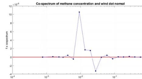
Figure 4. Average cospectrum of the outward-directed compo-nent of the observed wind and the methane concentration from 70 laps around a point source near San Antonio, Texas. The peak at 10−2Hz corresponds to the period of the circle.
Further evidence of this is shown in the average cospec-trum of the outward wind and concentration fluctuation ob-served in the flight loops in Fig. 4. Because the integral of the cospectrum yields the total flux (scalar and wind covariance), this function is useful for examining the contributions to the overall flux from each of the scales of motion (represented by aircraft speed divided by frequency). The results shown in Fig. 4 are from a CH4point source with an estimated emis-sion rate of 46±7 kg h−1 which was circled 70 times at a dimensionless radiusXof approximately 0.35. All cospectra of sampled sources have the same structure seen in Fig. 4: there is an obvious peak at the mean flight loop frequency (usually∼100 s period) followed by a smaller negative dip at higher frequencies within the meandering effluent plume. We believe this to be good evidence that our method cap-tures this important component of the overall flux away from the source, which cannot be obtained with a traditional mean wind and an integrated concentration enhancement measure-ment that is so often employed in airborne source estimates (Ryerson et al., 2001; White et al., 1976).
3.5 Choosing the downwind sampling distance
Figure 5. Dimensionless flux divergence profiles generated from averaging over 3 different WRF-LES runs using 30 time steps for each one. The horizontal flux per unit altitude (d=F /1z) is nor-malized by the boundary layer height,zi, and source strength,Q. The colored profiles are averages at various dimensionless dis-tances, R=0.1, 0.2, 0.3, and 0.4, and the gray areas represent 1 standard deviation about the mean. The horizontal dashed lines are the approximate lowest safe flight altitude.
To gain further insight into the second feature of the dis-persing plume, Fig. 5 shows the average horizontal flux di-vergence profiles derived from the three WRF-LES runs. Here we discuss a dimensionlessR, which is identical toX, to emphasize that this scaled downwind distance from the source is a radius of a flight loop. The flux divergence values are made dimensionless by the boundary layer height,zi, and the source emission rate,Q. Very close to the source, before the plume has had a chance to loft, the flux divergence profile exhibits a strong gradient below the minimum safe flight alti-tude, making that term difficult to measure directly, as shown in Fig. 5. Farther from the source, the signal becomes weaker with increasing altitude and eventually becomes increasingly influenced by entrainment fluxes. We therefore seek a sam-pling distance that is far enough to allow sufficient vertical lofting yet close enough so that plume crossings are easily observable against the background variability and instrument noise, and are not yet influenced by entrainment mixing.
Based on the simulation results presented in Fig. 5, we see the gradient below the lowest flight safe altitude typically be-comes very small for R >0.4, and therefore we attempt to target that distance to minimize the extrapolation error from the flight data to the surface. We do not currently measure all the necessary parameters to estimate R in flight (primarily the surface heat flux (w0θ0
v)0which is required to estimate
w∗). Instead, we estimatew∗based on the observed boundary layer height, standard deviation of wind speed, and a param-eterization forw∗=σu/0.6 (Caughey and Palmer, 1979).
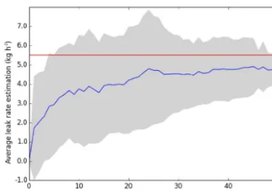
Figure 6.Rate of convergence toward the final leak rate estima-tion as a funcestima-tion of the number of loops for LES CASE UCD508. By 15 laps, the emissions estimate (blue line) has stabilized to 2.5 kg h−1compared to the actual leak rate (red line) of 2.9 kg h−1. Dimensionless distanceR=0.25, 50 realizations. Gray area repre-sents 1 SD (standard deviation).
3.6 Minimum number of passes
The atmospheric boundary layer is a turbulent medium, meaning that two passes across a plume at the same altitude and distance downwind will likely make very different mea-surements of the trace gases of interest. A natural question arises as to how many passes are required to develop a sta-tistically sound estimate of the emission rate. We investigate the number of passes required to obtain a statistically robust estimate using the WRF-LES results and a controlled release experiment. By calculating the horizontal flux divergences with a virtual airplane flying through the simulated tracer field, and then randomly sampling the flux divergences from each of the legs and plotting the resultant estimated emission rate as a function of the number of samples used, we obtain the results presented in Fig. 6. The gray region around the red line mean represents the standard deviation of estimates based on a random set of loops. Figure 7 shows results from an analysis of actual flight data from the controlled ethane re-lease test near Denver, Colorado, on 19 November 2014. It is evident from both the simulation data and the field data that a statistically stable estimate seems to be achieved somewhere between 20 and 25 loops around the source.
3.7 Discretization and altitude binning the flux divergence data
contri-Figure 7. Averaged LES estimates for the Aerodyne case. This leak shows a slightly higher number of laps before convergence (∼25 laps). This simulation was performed using the conditions for the Aerodyne controlled release near Denver, Colorado, on 19 November 2014.
butions times the sample length around each loop and then summing over the height intervals,
Qc=
∂m
∂t
+
Z I
Fc· ˆndS=
1m 1t
+ z=Zt
X
z=0 L
X
0
(ρ·un)·1s
!
·1z, (11)
whereρ is the scalar air density,unis the wind speed nor-mal to the flight path,1sis the distance covered during the 1 s time interval of each measurement, andLis the distance covered in one complete circuit. The outer summation sums each of the discrete vertical laps from the bottom (z=0) to the highest lap (z=zt). If all laps were sampled at equidis-tant altitudes, the total divergence could be calculated as the average divergence of all laps multiplied by the top altitude. However, because there is greater horizontal transport and variability at lower altitudes, as demonstrated by the widen-ing standard deviations approachwiden-ing the surface in the theo-retical flux divergence profiles shown in Fig. 4, more sam-pling laps at lower altitudes increase the statistical validity of the largest horizontal transport values. To ensure that all altitudes are nearly equally weighted, we divide the verti-cal range into six equally spaced bins, save for the lowest bin which is extended to the surface, and then average the measurements from the laps within each bin. The total emis-sion is the sum of the flux times the path length in each bin multiplied by the bin width. We also performed six flights where we sampled equally at all altitudes to allow for com-parison of the direct average vs. the binned results, and in all of these flights the values derived by the two methods agreed to within 5 %.
3.8 Error analysis
Our method assumes a stationary emission source. The leg-to-leg variability is primarily driven by the stochastic nature of turbulence (e.g., we may sample the plume on one lap and miss it on another). By aggregating the laps into verti-cal bins, we can use the standard deviation of the horizontal fluxes within each bin as an estimate of the uncertainty within that bin. Then the total uncertainty in the estimate of the flux divergence is simply estimated by adding up the individual bin uncertainties in quadrature. The first term on the rhs of Eq. (6) is the time rate of change of the scalar mass within the cylindrical flight volume. This storage term is estimated by performing a least squares fit of the methane density with time and altitude. The resulting uncertainty in the time rate of change is then combined (summed in quadrature) with the uncertainty from the altitude bins to achieve a total uncer-tainty in the measurement.
4 Results and discussion
We use measurements from three sets of flights to character-ize the accuracy of this estimation method. We flew 2 days measuring an controlled ethane release provided by Aero-dyne Research, Inc., 4 days measuring a controlled natu-ral gas release provided by the Pacific Gas & Electric Com-pany (PG & E), and six power plant flights where our esti-mates are compared with reported hourly power plant CO2 emissions.
4.1 Controlled ethane releases
Table 2.Controlled ethane releases.
Experiment Date Laps Released Estimated Released Estimated Ethane
location CH4 CH4 C2H6 C2H6 difference
kg h−1 kg h−1 kg h−1 kg h−1
Colorado 19 Nov 2014 50 0.0 −0.1±0.3 5.5±0.5 5.6±2.9 +2 % Arkansas 3 Oct 2015 19 0.0 −3.4±12.3 8.1±0.8 10.0±6.1 +24 %
Table 3.Controlled natural gas release.
Experiment Date Laps Released Estimated Released Estimated Methane
location CH4 CH4 C2H6 C2H6 difference
kg h−1 kg h−1 kg h−1 kg h−1
Rio Vista 3 Nov 2014 37 13.9±2.8 12.8±8.5 1.2±0.5 0.6±0.4 −8 % Rio Vista 4 Nov 2014 27 13.9±2.8 11.5±3.2 1.2±0.5 0.5±0.3 −17 %
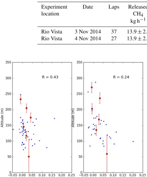
Figure 8.Ethane horizontal transport profiles for the Aerodyne con-trolled releases near Denver, Colorado, on 19 November 2014 ((a)) and in Bee Branch, Arkansas, on 3 October 2015 ((b)). Blue dots represent individual flight loop measurements and the red circles represent the bin average values for altitude intervals represented by the red bars.
A significant upwind ethane source was observed during the Arkansas experiment. This source was evident on roughly half of the upwind passes, suggesting that techniques which rely on a limited number of upwind passes to characterize the background could have a large random error and thus erro-neously estimate the upwind source strength. A similar prob-lem would affect those techniques that employ a downwind transect, using the edges of that transect lying outside the plume to estimate the background concentration. These ob-servations demonstrate the complication (and bias) that can arise from nearby sources. Since this method integrates all the emission sources in the area within the flight circle and a
small distance upwind of the circle depending on the vertical mixing, estimates from Gauss’s method may be biased high if there are sources within that area. The average error of the two ethane releases is 13 %.
4.2 Controlled natural gas releases
In conjunction with PG & E, we performed two sets of 2-day ground-level controlled release experiments from exist-ing PG & E facilities, exactly 1 year apart. The first set was performed southeast of Sacramento near the town of Rio Vista, CA at the Rio Vista “Y” station and the second set near Bakersfield, CA. For the Rio Vista test, the release rate was not calibrated with a flow meter but, based on the size of the orifice and the upstream pressure, the release rate was es-timated at 15.2±1.5 kg h−1. This release rate is an estimate of the total gas being released which is a combination of pri-marily CH4 and C2H6. We use the regression fit of ethane to methane (averaging 0.085 by mass) to estimate the actual release rate of each scalar.
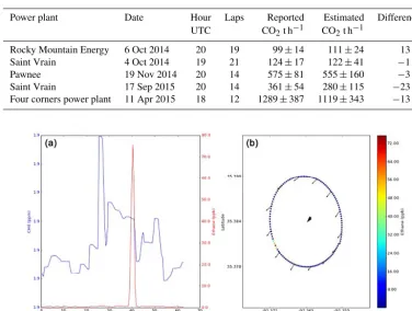
Table 4.Power plant estimates. The mid-point of the measurements (Hour UTC) is indicated in the third column (Hour). The reported emissions from the hour before to the hour after that time were averaged to derive the “Reported” emissions in column 5. Emissions are reported in units of metric tons (t) per hour.
Power plant Date Hour Laps Reported Estimated Difference
UTC CO2t h−1 CO2t h−1
Rocky Mountain Energy 6 Oct 2014 20 19 99±14 111±24 13 %
Saint Vrain 4 Oct 2014 19 21 124±17 122±41 −1 %
Pawnee 19 Nov 2014 20 14 575±81 555±160 −3 %
Saint Vrain 17 Sep 2015 20 14 361±54 280±115 −23 %
Four corners power plant 11 Apr 2015 18 12 1289±387 1119±343 −13 %
Figure 9. (a)Time series of methane (blue) and ethane (red) along with(b)the geographic distribution of ethane (color bar) and instantaneous winds (arrows) from a single flight loop during the second controlled ethane release.
4.3 Power plant flights
Power plants in the US are required to report CO2 emis-sions to United States Environmental Protection Agency (EPA; https://ampd.epa.gov/ampd) on an hourly basis. The accuracy of the reported CO2 emissions has been deter-mined to be ±10.8–11.0 % based on reported US aver-age differences between Energy Information Administra-tion (EIA) fuel-based estimates and EPA continuous emis-sion monitoring-based estimates (Ackerman and Sundquist, 2008; Peischl et al., 2010; Quick, 2014). Also, Peischl et al. (2010) determined an accuracy of power plants reporting CO2emissions in Texas of±14.0 % based on differences be-tween observed downwind SO2/CO2and NOx/CO2 emis-sion ratios and those reported via EPA continuous emisemis-sion monitoring (Peischl et al., 2010). Here, we use the slightly larger uncertainty from Peischl et al. (2010). Power plant emissions are “hot” gases and very buoyant, in contrast to a surface emission source that is typically not buoyant. An additional uncertainty arises from temporal emission vari-ability (hourly averaged reported CO2 emissions vs.<1 h power plant flights that may cover parts of two reported con-secutive hourly values). We estimate the total reported
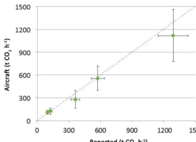
uncer-tainty by summing in quadrature the Peischl estimate and the relative difference between two reported consecutive hourly CO2 emission values closest to the time of the power plant sampling. The aircraft frequently encountered power plants during oil and gas monitoring campaigns, but usually did not have the flight time to perform a full emissions characteriza-tion of the power plant. Here we limit our comparison to days when the aircraft performed a minimum of 10 laps around the plant, thus excluding the quick fly-bys where uncertain-ties would be unacceptably large. The results are presented in Table 4 and indicate very good agreement between Gauss’s method and the reported CO2 emissions with the averaged difference being 10.6 %. A comparison plot of the reported vs. measured CO2emissions is shown in Fig. 10. The aver-age difference between the reported and measured emissions for the five power plants is 11 %.
5 Conclusion
ac-Figure 10.Comparison of aircraft vs. reported power plant emis-sions.
curate determination of the location and magnitude of a given emission site. The main uncertainty arises from the effluent below the lowest flight altitude, but this is minimized by tar-geting a downwind distance determined by LES studies to provide very little change in the plume flux divergence from the lowest loop to the ground. In addition to the controlled release experiments, hundreds of sites have been measured using this technique with varying levels of success. Ideal con-ditions include flat terrain, ample sunlight to promote vertical mixing, consistent winds, and no nearby competing sources. Under optimal conditions we have demonstrated that mea-surement uncertainties are quite low, often better than 10 %. As the conditions deteriorate from the ideal to situations in-volving complex terrain, variable winds or nearby upwind sources, measured uncertainties can increase to be as large or larger than the emission estimates themselves. In the worst case of stably stratified conditions (winter or nighttime), for instance, the lack of vertical mixing may preclude the trace gases emitted at the surface from reaching the minimum safe flight altitude. Complex terrain provides a challenge to the method because the aircraft is unable to maintain a constant altitude above the ground. A possible future refinement of this technique to be applied in complex terrain would be to fit the measurements of both wind and mixing ratio to a uniform 3-D surface surrounding the source, where the grid passes through the terrain and then integrate the flux normal to this irregular virtual flight path. This would not assume level loop flight legs and would, in principle, account for individual loops being flown at differing altitudes and thus more closely track mass continuity near the terrain elevation.
Data availability. Data are available upon request by the corre-sponding author.
Competing interests. The authors declare that they have no conflict of interest.
Acknowledgements. Funding for this study provided by the California Energy Commission (CEC) and the US Department of Energy (DOE). Funding for the Denver and Arkansas portion of this work was provided by RPSEA/NETL contract no. 12122-95/DE-AC26-07NT42677 to the Colorado School of Mines. Cost sharing was provided by Colorado Energy Research Collaboratory, the National Oceanic and Atmospheric Administration Climate Pro-gram Office, the National Science Foundation (CBET-1240584), Southwestern Energy, XTO, Chevron, Statoil, and the American Gas Association, many of whom also provided operational data and/or site access. We also thank Shuhua Chen for assistance with the WRF-LES code modifications and advice. The National Center for Atmospheric Research is sponsored by the National Science Foundation. This work was supported in part by the NOAA AC4 program under grant NA14OAR0110139 and the Bureau of Land Management, grant L15PG00058. We thank Ying Pan for her significant contribution to our understanding of the negative horizontal scalar flux.
Edited by: Andre Butz
Reviewed by: three anonymous referees
References
Ackerman, K. V. and Sundquist, E. T.: Comparison of two US power-plant carbon dioxide emissions data sets, Environ. Sci. Technol., 42, 5688–5693, 2008.
Alfieri, S., Amato, U., Carfora, M. F., Esposito, M., and Magliulo, V.: Quantifying trace gas emissions from composite landscapes: A mass-budget approach with aircraft measurements, Atmos. En-viron., 44, 1866–1876, 2010.
Bergamaschi, P., Krol, M., Dentener, F., Vermeulen, A., Meinhardt, F., Graul, R., Ramonet, M., Peters, W., and Dlugokencky, E. J.: Inverse modelling of national and European CH4emissions us-ing the atmospheric zoom model TM5, Atmos. Chem. Phys., 5, 2431–2460, https://doi.org/10.5194/acp-5-2431-2005, 2005. Beswick, K. M., Simpson, T. W., Fowler, D., Choularton, T. W.,
Gallagher, M. W., Hargreaves, K. J., Sutton, M. A., and Kaye, A.: Methane emissions on large scales, Atmos. Environ., 32, 3283– 3291, 1998.
Caughey, S. J. and Palmer, S. G.: Some aspects of turbulence struc-ture through the depth of the convective boundary-layer, Q. J. Roy. Meteorol. Soc., 105, 811–827, 1979.
Caulton, D. R., Shepson, P. B., Santoro, R. L., Sparks, J. P., Howarth, R. W., Ingraffea, A. R., Cambaliza, M. O. L., Sweeney, C., Karion, A., Davis, K. J., Stirm, B. H., Montzka, S. A., and Miller, B. R.: Toward a better understanding and quantification of methane emissions from shale gas development, P. Natl. Acad. Sci. USA, 111, 6237–6242, 2014.
Chang, R. Y. W., Miller, C. E., Dinardo, S. J., Karion, A., Sweeney, C., Daube, B. C., Henderson, J. M., Mountain, M. E., Eluszkiewicz, J., Miller, J. B., Bruhwiler, L. M. P., and Wofsy, S. C.: Methane emissions from Alaska in 2012 from CARVE air-borne observations, P. Natl. Acad. Sci. USA, 111, 16694–16699, 2014.
Conley, S. A., Faloona, I. C., Lenschow, D. H., Karion, A., and Sweeney, C.: A Low-Cost System for Measuring Horizontal Winds from Single-Engine Aircraft, J. Atmos. Ocean. Tech., 31, 1312–1320, 2014.
Crosson, E. R.: A cavity ring-down analyzer for measuring atmo-spheric levels of methane, carbon dioxide, and water vapor, Appl. Phys. B, 92, 403–408, 2008.
Czepiel, P. M., Mosher, B., Harriss, R. C., Shorter, J. H., McManus, J. B., Kolb, C. E., Allwine, E., and Lamb, B. K.: Landfill methane emissions measured by enclosure and atmospheric tracer meth-ods, J. Geophys. Res.-Atmos., 101, 16711–16719, 1996. Denmead, O. T., Harper, L. A., Freney, J. R., Griffith, D. W. T.,
Le-uning, R., and Sharpe, R. R.: A mass balance method for non-intrusive measurements of surface-air trace gas exchange, At-mos. Environ., 32, 3679–3688, 1998.
Gallagher, M. W., Choularton, T. W., Bower, K. N., Stromberg, I. M., Beswick, K. M., Fowler, D., and Hargreaves, K. J.: Measure-ments of methane fluxes on the landscape scale form a wetland area in North Scotland, Atmos. Environ., 28, 2421–2430, 1994. Gerbig, C., Lin, J. C., Wofsy, S. C., Daube, B. C., Andrews, A.
E., Stephens, B. B., Bakwin, P. S., and Grainger, C. A.: Toward constraining regional-scale fluxes of CO2 with atmospheric ob-servations over a continent: 2. Analysis of COBRA data using a receptor-oriented framework, J. Geophys. Res.-Atmos., 108, 4756, https://doi.org/10.1029/2002JD003018, 2003.
Gordon, M., Li, S.-M., Staebler, R., Darlington, A., Hayden, K., O’Brien, J., and Wolde, M.: Determining air pollutant emission rates based on mass balance using airborne measurement data over the Alberta oil sands operations, Atmos. Meas. Tech., 8, 3745–3765, https://doi.org/10.5194/amt-8-3745-2015, 2015. Hacker, J. M., Chen, D. L., Bai, M., Ewenz, C., Junkermann, W.,
Lieff, W., McManus, B., Neininger, B., Sun, J. L., Coates, T., Denmead, T., Flesch, T., McGinn, S., and Hill, J.: Using airborne technology to quantify and apportion emissions of CH4and NH3 from feedlots, Animal Prod. Sci., 56, 190–203, 2016.
Hiller, R. V., Neininger, B., Brunner, D., Gerbig, C., Bretscher, D., Kunzle, T., Buchmann, N., and Eugster, W.: Aircraft-based CH4 flux estimates for validation of emissions from an agriculturally dominated area in Switzerland, J. Geophys. Res.-Atmos., 119, 4874–4887, 2014.
Hirsch, A. I., Michalak, A. M., Bruhwiler, L. M., Peters, W., Dlugokencky, E. J., and Tans, P. P.: Inverse mod-eling estimates of the global nitrous oxide surface flux from 1998–2001, Global Biogeochem. Cy., 20, GB1008, https://doi.org/10.1029/2004GB002443, 2006.
Kalthoff, N., Corsmeier, U., Schmidt, K., Kottmeier, C., Fiedler, F., Habram, M., and Slemr, F.: Emissions of the city of Augsburg determined using the mass balance method, Atmos. Environ., 36, S19–S31, 2002.
Karion, A., Sweeney, C., Petron, G., Frost, G., Hardesty, R. M., Kofler, J., Miller, B. R., Newberger, T., Wolter, S., Banta, R., Brewer, A., Dlugokencky, E., Lang, P., Montzka, S. A., Schnell, R., Tans, P., Trainer, M., Zamora, R., and Conley, S.: Methane emissions estimate from airborne measurements over a western United States natural gas field, Geophys. Res. Lett., 40, 4393– 4397, 2013.
Karion, A., Sweeney, C., Kort, E. A., Shepson, P. B., Brewer, A., Cambaliza, M., Conley, S. A., Davis, K., Deng, A. J., Hardesty, M., Herndon, S. C., Lauvaux, T., Lavoie, T., Lyon, D.,
New-berger, T., Petron, G., Rella, C., Smith, M., Wolter, S., Yacov-itch, T. I., and Tans, P.: Aircraft-Based Estimate of Total Methane Emissions from the Barnett Shale Region, Environ. Sci. Technol., 49, 8124–8131, 2015.
Lamb, B. K., McManus, J. B., Shorter, J. H., Kolb, C. E., Mosher, B., Harriss, R. C., Allwine, E., Blaha, D., Howard, T., Guenther, A., Lott, R. A., Siverson, R., Westberg, H., and Zimmerman, P.: Development of atmospheric tracer methods to measure methane emissions form natural-gas facilities and urban areas, Environ. Sci. Technol., 29, 1468–1479, 1995.
Lavoie, T. N., Shepson, P. B., Cambaliza, M. O. L., Stirm, B. H., Karion, A., Sweeney, C., Yacovitch, T. I., Herndon, S. C., Lan, X., and Lyon, D.: Aircraft-Based Measurements of Point Source Methane Emissions in the Barnett Shale Basin, Environ. Sci. Technol., 49, 7904–7913, 2015.
Lenschow, D. H., Savic-Jovcic, V., and Stevens, B.: Divergence and vorticity from aircraft air motion measurements, J. Atmos. Ocean. Tech., 24, 2062–2072, 2007.
Leuning, R., Freney, J. R., Denmead, O. T., and Simpson, J. R.: A sampler for measuring atmospheric ammonia flux, Atmos. Envi-ron., 19, 1117–1124, 1985.
Mays, K. L., Shepson, P. B., Stirm, B. H., Karion, A., Sweeney, C., and Gurney, K. R.: Aircraft-Based Measurements of the Carbon Footprint of Indianapolis, Environ. Sci. Technol., 43, 7816–7823, 2009.
Miller, J. B., Lehman, S. J., Montzka, S. A., Sweeney, C., Miller, B. R., Karion, A., Wolak, C., Dlugokencky, E. J., Southon, J., Turnbull, J. C., and Tans, P. P.: Linking emissions of fos-sil fuel CO2and other anthropogenic trace gases using atmo-spheric (CO2)-C-14, J. Geophys. Res.-Atmos., 117, D08302, https://doi.org/10.1029/2011JD017048, 2012.
Miller, S. M., Wofsy, S. C., Michalak, A. M., Kort, E. A., Andrews, A. E., Biraud, S. C., Dlugokencky, E. J., Eluszkiewicz, J., Fis-cher, M. L., Janssens-Maenhout, G., Miller, B. R., Miller, J. B., Montzka, S. A., Nehrkorn, T., and Sweeney, C.: Anthropogenic emissions of methane in the United States, P. Natl. Acad. Sci. USA, 110, 20018–20022, 2013.
Muhle, S., Balsam, I., and Cheeseman, C. R.: Comparison of carbon emissions associated with municipal solid waste management in Germany and the UK, Resour. Conserv. Recycl., 54, 793–801, 2010.
Neef, L., van Weele, M., and van Velthoven, P.: Optimal estimation of the present-day global methane budget, Global Biogeochem. Cy., 24, GB4024, https://doi.org/10.1029/2009GB003661, 2010. Nisbet, E. and Weiss, R.: Top-Down Versus Bottom-Up, Science,
328, 1241–1243, 2010.
Pan, Y., Chamecki, M., and Isard, S. A.: Large-eddy simulation of turbulence and particle dispersion inside the canopy roughness sublayer, J. Fluid Mech., 753, 499–534, 2014.
Peischl, J., Ryerson, T. B., Holloway, J. S., Parrish, D. D., Trainer, M., Frost, G. J., Aikin, K. C., Brown, S. S., Dube, W. P., Stark, H., and Fehsenfeld, F. C.: A top-down analy-sis of emissions from selected Texas power plants during Tex-AQS 2000 and 2006, J. Geophys. Res.-Atmos., 115, D16303, https://doi.org/10.1029/2009JD013527, 2010.
P. M., Novelli, P. C., Santoni, G. W., Trainer, M., Wofsy, S. C., and Parrish, D. D.: Quantifying sources of methane using light alkanes in the Los Angeles basin, California, J. Geophys. Res.-Atmos., 118, 4974-4990, 2013.
Petron, G., Karion, A., Sweeney, C., Miller, B. R., Montzka, S. A., Frost, G. J., Trainer, M., Tans, P., Andrews, A., Kofler, J., Helmig, D., Guenther, D., Dlugokencky, E., Lang, P., New-berger, T., Wolter, S., Hall, B., Novelli, P., Brewer, A., Conley, S., Hardesty, M., Banta, R., White, A., Noone, D., Wolfe, D., and Schnell, R.: A new look at methane and nonmethane hydro-carbon emissions from oil and natural gas operations in the Col-orado Denver-Julesburg Basin, J. Geophys. Res.-Atmos., 119, 6836–6852, 2014.
Quick, J. C.: Carbon dioxide emission tallies for 210 U.S. coal-fired power plants: A comparison of two accounting methods, J. Air Waste Manage. Assoc., 64, 73–79, 2014.
Raupach, M. R. and Legg, B. J.: The uses and limitations of flux– gradient relationships in micrometeorology, Agr. Water Manage., 8, 119–131, 1984.
Ritter, J. A., Barrick, J. D. W., Watson, C. E., Sachse, G. W., Gre-gory, G. L., Anderson, B. E., Woerner, M. A., and Collins, J. E.: Airborne boundary-layer flux measurements of trace species over Canadian boreal forest and northern wetland regions, J. Geophys. Res.-Atmos., 99, 1671–1685, 1994.
Roscioli, J. R., Yacovitch, T. I., Floerchinger, C., Mitchell, A. L., Tkacik, D. S., Subramanian, R., Martinez, D. M., Vaughn, T. L., Williams, L., Zimmerle, D., Robinson, A. L., Hern-don, S. C., and Marchese, A. J.: Measurements of methane emissions from natural gas gathering facilities and processing plants: measurement methods, Atmos. Meas. Tech., 8, 2017– 2035, https://doi.org/10.5194/amt-8-2017-2015, 2015.
Ryerson, T. B., Buhr, M. P., Frost, G. J., Goldan, P. D., Holloway, J. S., Hubler, G., Jobson, B. T., Kuster, W. C., McKeen, S. A., Par-rish, D. D., Roberts, J. M., Sueper, D. T., Trainer, M., Williams, J., and Fehsenfeld, F. C.: Emissions lifetimes and ozone for-mation in power plant plumes, J. Geophys. Res.-Atmos., 103, 22569–22583, 1998.
Ryerson, T. B., Trainer, M., Holloway, J. S., Parrish, D. D., Huey, L. G., Sueper, D. T., Frost, G. J., Donnelly, S. G., Schauffler, S., Atlas, E. L., Kuster, W. C., Goldan, P. D., Hubler, G., Meagher, J. F., and Fehsenfeld, F. C.: Observations of ozone formation in power plant plumes and implications for ozone control strategies, Science, 292, 719–723, 2001.
Stull, R. B.: An Introduction to Boundary Layer Meteorology, Kluwer Academic Publishers, Norwell, MA, 1988.
Taylor, G. I.: Diffusion by Continuous Movements, Proc. Lond. Math. Soc., s2-20, 196–212, 1922.
Tratt, D. M., Buckland, K. N., Hall, J. L., Johnson, P. D., Keim, E. R., Leifer, I., Westberg, K., and Young, S. J.: Airborne visu-alization and quantification of discrete methane sources in the environment, Remote Sensing Environ., 154, 74–88, 2014. Turnbull, J. C., Karion, A., Fischer, M. L., Faloona, I.,
Guilder-son, T., Lehman, S. J., Miller, B. R., Miller, J. B., Montzka, S., Sherwood, T., Saripalli, S., Sweeney, C., and Tans, P. P.: Assess-ment of fossil fuel carbon dioxide and other anthropogenic trace gas emissions from airborne measurements over Sacramento, California in spring 2009, Atmos. Chem. Phys., 11, 705–721, https://doi.org/10.5194/acp-11-705-2011, 2011.
Wecht, K. J., Jacob, D. J., Frankenberg, C., Jiang, Z., and Blake, D. R.: Mapping of North American methane emissions with high spatial resolution by inversion of SCIAMACHY satellite data, J. Geophys. Res.-Atmos., 119, 7741–7756, 2014.
Weil, J. C.: Dispersion in the Convective Boundary Layer, in: Lec-tures on Air Pollution Modeling, edited by: Venkatram, A. and Wyngaard, J. C., American Meteorological Society, Boston, MA, 1988.
Weil, J. C., Sullivan, P. P., Patton, E. G., and Moeng, C.-H.: Statisti-cal Variability of Dispersion in the Convective Boundary Layer: Ensembles of Simulations and Observations, Bound.-Lay. Mete-orol., 145, 185–210, 2012.
White, W. H., Anderson, J. A., Blumenthal, D. L., Husar, R. B., Gillani, N. V., Husar, J. D., and Wilson Jr., W. E.: Formation and Transport of Secondary Air Pollutants: Ozone and Aerosols in the St. Louis Urban Plume, Science, 194, 187–189, 1976. Wilczak, J. M. and Bedard, A. J.: A new turbulence
microbarome-ter and its evaluation using the budget of horizontal heat flux, J. Atmos. Ocean. Tech., 21, 1170–1181, 2004.
Willis, G. E. and Deardorff, J. W.: Laboratory model of diffusion into convective planetary bounday-layer, Q. J. Roy. Meteorol. Soc., 102, 427–445, 1976.
Wilson, J. D. and Shum, W. K. N.: A reexamination of the integrated horizontal flux method of estimating volatilization from circular plots, Agr. Forest Meteorol., 57, 281–295, 1992.
Wratt, D. S., Gimson, N. R., Brailsford, G. W., Lassey, K. R., Brom-ley, A. M., and Bell, M. J.: Estimating regional methane emis-sions from agriculture using aircraft measurements of concentra-tion profiles, Atmos. Environ., 35, 497–508, 2001.
Wyngaard, J. C.: Turbulence in the Atmosphere, Cambridge Uni-versity Press, Cambridge, 2010.
Wyngaard, J. C. , Coté, O. R., and Izumi, Y.: Local free convection, similarity, and the budgets of shear stress and heat flux, J. Atmos. Sci., 28, 1171–1182, 1971.
Yacovitch, T. I., Herndon, S. C., Roscioli, J. R., Floerchinger, C., McGovern, R. M., Agnese, M., Petron, G., Kofler, J., Sweeney, C., Karion, A., Conley, S. A., Kort, E. A., Nahle, L., Fischer, M., Hildebrandt, L., Koeth, J., McManus, J. B., Nelson, D. D., Zah-niser, M. S., and Kolb, C. E.: Demonstration of an Ethane Spec-trometer for Methane Source Identification, Environ. Sci. Tech-nol., 48, 8028–8034, 2014.