www.atmos-meas-tech.net/10/247/2017/ doi:10.5194/amt-10-247-2017
© Author(s) 2017. CC Attribution 3.0 License.
Evaluation of single and multiple Doppler lidar techniques
to measure complex flow during the XPIA field campaign
Aditya Choukulkar1,2, W. Alan Brewer2, Scott P. Sandberg2, Ann Weickmann1,2, Timothy A. Bonin1,2,
R. Michael Hardesty1,2, Julie K. Lundquist3,4, Ruben Delgado5, G. Valerio Iungo6, Ryan Ashton6, Mithu Debnath6, Laura Bianco1,7, James M. Wilczak7, Steven Oncley8, and Daniel Wolfe7
1Cooperative Institute for Research in Environmental Sciences, Boulder, CO, USA
2Chemical Sciences Division, National Oceanic and Atmospheric Administration, Boulder, CO, USA 3Department of Atmospheric and Oceanic Sciences, University of Colorado Boulder, CO, USA 4National Renewable Energy Laboratory, Golden, CO, USA
5Atmospheric Physics Department, University of Maryland Baltimore County, MD, USA 6Department of Mechanical Engineering, University of Texas at Dallas, Richardson, TX, USA 7Physical Sciences Division, National Oceanic and Atmospheric Administration, Boulder, CO, USA 8National Center for Atmospheric Research, Boulder, CO, USA
Correspondence to:Aditya Choukulkar ([email protected])
Received: 1 October 2016 – Published in Atmos. Meas. Tech. Discuss.: 10 October 2016 Revised: 21 December 2016 – Accepted: 22 December 2016 – Published: 23 January 2017
Abstract. Accurate three-dimensional information of wind flow fields can be an important tool in not only visualizing complex flow but also understanding the underlying physical processes and improving flow modeling. However, a thor-ough analysis of the measurement uncertainties is required to properly interpret results. The XPIA (eXperimental Plane-tary boundary layer Instrumentation Assessment) field cam-paign conducted at the Boulder Atmospheric Observatory (BAO) in Erie, CO, from 2 March to 31 May 2015 brought together a large suite of in situ and remote sensing mea-surement platforms to evaluate complex flow meamea-surement strategies.
In this paper, measurement uncertainties for different sin-gle and multi-Doppler strategies using simple scan geome-tries (conical, vertical plane and staring) are investigated. The tradeoffs (such as time–space resolution vs. spatial coverage) among the different measurement techniques are evaluated using co-located measurements made near the BAO tower. Sensitivity of the single-/multi-Doppler measurement uncer-tainties to averaging period are investigated using the sonic anemometers installed on the BAO tower as the standard ref-erence. Finally, the radiometer measurements are used to par-tition the measurement periods as a function of atmospheric
stability to determine their effect on measurement uncer-tainty.
It was found that with an increase in spatial coverage and measurement complexity, the uncertainty in the wind mea-surement also increased. For multi-Doppler techniques, the increase in uncertainty for temporally uncoordinated mea-surements is possibly due to requiring additional assump-tions of stationarity along with horizontal homogeneity and less representative line-of-sight velocity statistics. It was also found that wind speed measurement uncertainty was lower during stable conditions compared to unstable conditions.
1 Introduction
line-of-sight (LOS) velocity or radial velocity given in Eq. (1).
Vr=usinθcosφ+vcosθcosφ+wsinφ, (1)
whereVr is the LOS velocity,u,v,ware the velocity
com-ponents in the east–west direction, the north–south direction, and in the vertical, respectively, andθandφare the azimuth and elevation angles, respectively. In order to derive the two-dimensional (2-D) or three-two-dimensional (3-D) wind velocity the use of suitable measurement strategies and/or velocity re-trieval algorithms is required.
The 2-D and 3-D wind measurements from Doppler lidars are useful in various fields of study such as boundary layer meteorology (Fernando et al., 2015; Vanderwende et al., 2015), air quality (Barlow et al., 2011; Collier et al., 2005), wind energy research (Banta et al., 2015; Käsler et al., 2010; Mikkelsen, 2014; Newsom et al., 2015) and others. The sim-plest techniques to derive a profile of wind speed and di-rection using a single-Doppler lidar are the velocity azimuth display (VAD) technique (Browning and Wexler, 1968) and the Doppler beam swinging (DBS) technique (Strauch et al., 1984). These techniques assume horizontal homogeneity of the wind in the measurement volume to estimate the profile of wind speed and direction. Other techniques such as the velocity volume processing (Waldteufel and Corbin, 1979) and the “arc scan” technique (Wang et al., 2015) limit the assumption of horizontal homogeneity to smaller volumes within the lidar scans or to certain azimuth ranges, respec-tively, allowing one to better preserve the spatial variability information at the expense of increased uncertainty in the wind retrieval, especially when the wind direction is perpen-dicular to the scan sector (Krishnamurthy et al., 2013).
A common method to make wind-field measurements without assumption of spatial homogeneity is through multi-Doppler techniques. “Virtual towers” (Calhoun et al., 2006) use multiple Doppler lidars to interrogate a common vol-ume in space in a temporally coordinated fashion, iterat-ing through several height in order to create a wind profile. Several configurations of multi-Doppler scanning have been tested to quantify the skill in deriving 2-D and 3-D wind fields. For example, co-planar RHI scans were used to study flows in mountain valleys (Hill et al., 2010) and within a meteor crater (Cherukuru et al., 2015), and co-planar con-ical scans (PPIs) have been used to study coherent struc-tures (Newsom et al., 2008; Träumner et al., 2015) and wind turbine wakes (Vollmer et al., 2015). Three-dimensional wind-field measurements made using dual-Doppler intersect-ing RHI scans and usintersect-ing continuity to estimate the verti-cal velocity were used to study flow upstream and down-stream of a utility-scale wind turbine (Newsom et al., 2015). Three-dimensional wind and turbulence measurements using fully coordinated short-range continuous wave triple lidars (Mikkelsen et al., 2008; Simley et al., 2016) and long-range triple lidar scanning (Berg et al., 2015; Vasiljevi´c et al., 2016) have been demonstrated to provide high quality measure-ments of complex flow. In addition, manually coordinated
triple lidar measurements (Wang et al., 2016) were also tested and showed promise in measuring the 3-D wind fields oper-ationally. The Lower Atmospheric Boundary Layer Experi-ment (LABLE) validated wind and turbulence measureExperi-ments from triple-Doppler lidar measurements (Klein et al., 2015; Newman et al., 2016).
In addition to multi-Doppler approaches to measuring complex flow, several techniques enable wind-field retrievals from single-Doppler lidars, which resolve the spatial vari-ability measured by the lidar. For example, the optimal inter-polation (OI) technique allows 2-D wind-field retrievals on azimuthal scans (Choukulkar et al., 2012) without assump-tion of homogeneity of the wind field. In addiassump-tion, variaassump-tional methods can determine the wind fields from single or multi-ple Dopmulti-pler lidars (Chan and Shao, 2007; Drechsel et al., 2009; Newsom et al., 2008).
The choice of the measurement strategy and the retrieval algorithms comes with assumptions inherent to their pro-cess which need to be properly understood to interpret the measurements made. Several studies have been conducted to evaluate the measurement accuracy of the various single and multi-Doppler techniques. For example, measurement uncertainties in wind measurements made using the DBS technique in complex terrain were investigated by Bingöl et al. (2009) while Lundquist et al. (2015) studied the uncer-tainties in wind measurements using the DBS technique in presence of complex flow by simulating lidar measurements within a wind turbine wake using a wind field created with large-eddy simulation. Wind-field measurements made using the virtual tower technique have been validated (Damian et al., 2014; Gunter et al., 2015) to show high skill in measuring 2-D wind fields and Stawiarski et al. (2013) did a detailed er-ror analysis of dual Doppler co-planar PPI technique. Uncer-tainties in 3-D wind-field retrievals using triple-Doppler lidar techniques have also been investigated. For example, Mann et al. (2009), Fuertes et al. (2014) and Newman et al. (2016) present a detailed analysis of 3-D winds and turbulence mea-surements made using staring triple-Doppler meamea-surements, while Berg et al. (2015) present validation of 3-D wind mea-surements made through continuous scanning.
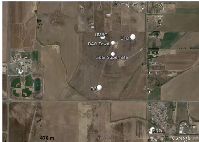
Figure 1.Scanning Doppler lidar deployment location during the XPIA field campaign.
addition, the tradeoffs in terms of measurement precision, spatial coverage and temporal resolution between the vari-ous measurement techniques are also discussed. The mea-surement techniques discussed in this paper are limited to using simple scan geometries such PPI, RHI and stare scans. However, as most commercially available lidar systems are limited to performing these scan modes, this paper discusses the possibilities available to such lidar systems. The paper is organized as follows: the experiment setup and measurement area is described in Sect. 2. Section 3 presents analysis of the LOS velocity uncertainty and Sect. 4 presents results from the validation of the different measurement techniques tested in XPIA. This is followed by a discussion of the results in Sect. 5. Concluding remarks are presented in Sect. 6.
2 Experiment setup
The XPIA field study, funded by the US Department of En-ergy (DOE) within the Atmosphere to electrons (A2e) pro-gram, had the goal to assess current capabilities for mea-suring complex flow in and near wind farms using remote sensing instrumentation. With this goal in mind, a large suite of instrumentation was deployed near the BAO (Kaimal and Gaynor, 1983) facility in Erie, CO. The instrumentation in-cluded six scanning Doppler lidars (four capable of coordi-nated scanning) and five vertically profiling lidars. Lundquist et al. (2016a) give a detailed description of the XPIA field study along with an overview of the instrumentation deploy-ment. Herein, for sake of brevity, only the details of the scanning lidar deployment used for testing the various
sin-gle and multi-Doppler measurements are described. These li-dars included two Leosphere 200S®scanning lidars (named D1 and D2) and the high-resolution Doppler lidar (HRDL) from the National Oceanic and Atmospheric Administra-tion (NOAA), one Leosphere 200S®scanning Doppler lidar from the University of Texas at Dallas (UTD) and one Leo-sphere 200S® from the University of Maryland Baltimore County (UMBC). Figure 1 shows the deployment locations of these scanning lidars with respect to the 300 m tall instru-mented BAO tower. The pulse width and time accumulation for each of the lidars used in the analysis presented in this paper is given in Table 1. All the wind measurement compar-isons presented in this paper are with respect to the measure-ments made by the southeast sonic anemometers installed on the BAO tower as the center of the lidar measurement volume (and the range gates) were always south of the BAO tower. The sonic anemometer data are filtered to remove tower wake effects using the criteria defined in McCaffrey et al. (2016).
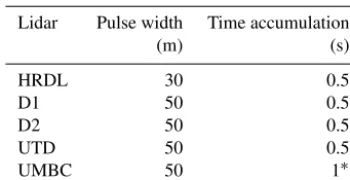
Table 1.Lidar operational parameters.
Lidar Pulse width Time accumulation
(m) (s)
HRDL 30 0.5
D1 50 0.5
D2 50 0.5
UTD 50 0.5
UMBC 50 1∗
∗Longer accumulation time was selected to ensure sufficient range (and hence coverage) during uncoordinated volume scans.
Table 2.Scanner pointing accuracy and repeatability estimates for the scanning Doppler lidars.
Lidar Pointing Repeatability Repeatability error (◦) in AZ (◦) in EL (◦)
HRDL < 0.1 ∼0.05 ∼0.05
D1 ∼0.15 0.01 0.05
D2 ∼0.15 0.01 0.05
UTD ∼0.15 Not determined Not determined UMBC ∼0.15 Not determined Not determined
scan initialization delay, the delay introduced due to each of the lidars scanning varying range of azimuths to reach the measurement location was characterized and accounted for during the scan strategy design for each of the measure-ment techniques evaluated. The net impact of all the pointing and time synchronization uncertainties is that all the systems could make measurements at a prescribed location at a given time with pointing uncertainty of less than 0.15◦ (approxi-mately ±2.5 m at 1 km range) and time uncertainty of less than 0.4 s.
In this paper, the following Doppler lidar measurement techniques will be discussed:
1. coordinated triple-Doppler virtual tower stares (VTS), 2. coordinated triple-Doppler sparse sampling scans, 3. uncoordinated triple-Doppler virtual tower, 4. uncoordinated multi-Doppler volume scan and
5. single-Doppler lidar wind retrieval using the optimal in-terpolation (OI) technique.
2.1 Coordinated triple-Doppler virtual tower stares The coordinated VTS scan pattern involves interrogating a common volume using multiple Doppler lidars at pre-defined heights at a given location to form a “virtual tower” (Cal-houn et al., 2006; Mann et al., 2009; Fuertes et al., 2014; Gunter et al., 2015; Newman et al., 2016). A schematic of
Table 3. Scan initialization delay estimates for the scanning Doppler lidars.
Lidar Scan initialization SD of the delay (s) delay (s)
HRDL 43.28a 0.42
D1 3.98 0.29
D2 3.81 0.3
UTD 0.79 0.3
UMBC Not applicableb Not applicable
aThe unusually long delay is due to the automatic scanner
calibration routine run at the beginning of each scan cycle.
bThis system did not have ability to trigger scans at prescribed
times.
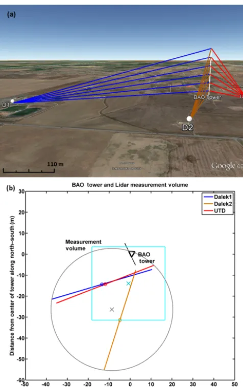
the triple lidar VTS scan tested during the XPIA field ex-periment is shown in Fig. 2a. Each of the three 200S lidars (D1, D2 and UTD) performed a temporally correlated 25 s stare at each of the six sonic anemometer levels (50 to 300 m with 50 m increments) and therefore creating a virtual tower of wind measurements every 3 min. The LOS velocities that fall within the common volume are least-squares fitted using Eq. (1) (Fuertes et al., 2014) to estimate the 3-D wind veloc-ity.
The common volume is defined as a square (cyan box in Fig. 2b), 35 m on a side and 10 m in the vertical centered at each of the sonic height levels with its center 10 m south of the southeast sonic anemometer on the BAO tower (this was the closest position to the tower that allowed overlapping measurements without blockage). As observed from Fig. 2b, the effective measurement volume (defined as the circle en-veloping the outermost range-gate points) is slightly larger with a diameter of 60 m. It is also seen from Fig. 2b that the look directions of D1 and UTD are close to 180◦apart. This non-ideal setup for triple-Doppler measurements was dictated by logistics of deployment. However, the UTD li-dar makes measurements with much steeper elevation angles compared to D1 and hence does provide additional informa-tion for wind retrieval.
Similar virtual towers were performed at two other loca-tions to compare with other instrumentation deployed during XPIA. Therefore the repeat period for these virtual towers discussed here is once every 10 min. The 25 s stare period was chosen to ensure that all three 200S lidars were measur-ing the common volume simultaneously. However, the 3-D wind retrieval was made using 5 s of spatially and temporally overlapping LOS velocity data.
Figure 2.The virtual tower stare (VTS) scan.(a)Schematic of the VTS technique. The blue, red and orange lines indicate beams from each of the three 200S lidars that make measurements at each sonic anemometer level.(b) Location and size of the common volume (cyan box) with respect to the BAO tower. The blue, red and orange lines are range gates from the three 200S lidars that fall within the common volume. The grey circle indicates the estimated measure-ment volume defined by the position of the range gates.
over a large enough area using contiguous volumes is the time required to simultaneously interrogate this area using coordinated scanning. The time required to complete a scan is determined by the data rate of the lidar systems, overlap period and the geometry defined by the instrument locations. Given the instrument locations during XPIA and data rate limitations of the 200S lidars, the time required to sample an area through contiguous measurement points would be too long to sample a feature sufficiently before it advected out of the measurement domain. Therefore, to reduce the time required to make such a measurement, sparse sampling strategies were considered. The sparse sampling technique discussed in this paper is called small checkerboard (SCB)
scan and the layout of this technique is shown in Fig. 3. The scanning strategy involved sampling a 3×3 grid covering a horizontal area of approximately 150 m×150 m and 100 m above the ground. The three lidars paused 5 s at each grid point and hence completed one SCB scan every 1 min. This measurement strategy was carried out using the D1, D2 and UTD scanning 200S lidars for a period of 9 days.
2.3 Uncoordinated triple-Doppler virtual tower This measurement technique is similar to the one explained in Sect. 2.1 in that three Doppler lidars scan a common vol-ume to make 3-D wind-field measurements. However, in or-der to reduce the time required to perform a virtual tower and increase the update rates, the lidars performed continu-ous temporally uncoordinated RHI scans at the BAO tower location. Each RHI scan takes 15 s to perform and hence a 3-D wind-field measurement can be made every 15 s, com-pared to 3 min required for the VTS technique. The tradeoff is that not all lidars are looking at the same volume simulta-neously. The 3-D wind field is estimated by least-squares fit-ting to Eq. (1) the LOS velocity measurements from the three 200S lidars (D1, D2 and UTD) that fall within the common volume (50 m on a side and 10 m in the vertical) and within a 15 s time window. The three 200S lidars performed inter-secting RHI scans at three locations (including near the BAO tower) for 20 min at each location before repeating the se-quence again. This measurement strategy was performed for a period of approximately 2 days.
2.4 Uncoordinated multi-Doppler volume scan
With the uncoordinated multi-Doppler measurement tech-nique, the constraint that multiple lidars need to interrogate a common volume simultaneously is removed allowing to speed up sampling of the domain of interest. In this measure-ment technique, five Doppler lidars (HRDL, D1, D2, UTD and UMBC) performed a set of complementary PPI scans that would ensure that at least two Doppler beams overlapped within each grid point (defined as 50 m on a side in the hori-zontal and 15 m in the vertical) within a 5 min update period. This scan strategy resulted in a grid which approximately 1.5 km×1 km in the horizontal and covered heights 30 m to 300 m above the ground with 15 m vertical resolution. A rep-resentation of the scans performed by each of the scanning lidars and the resulting grid is shown in Fig. 4.
Figure 3.Schematic of the small checkerboard (SCB) scan. The white outline shows the domain over which measurements are made and the blue squares indicate the locations of measurement volumes interrogated by the scanning Doppler lidars.
the Doppler lidars further away from the domain of interest so that shallower elevation PPI scans can be employed which can help cover larger areas with faster update rates.
2.5 Single-Doppler velocity retrievals
The single-Doppler retrieval technique investigated in this paper is the OI technique (Choukulkar et al., 2012). The OI technique allows retrieval of 2-D wind fields over PPI scans without assumption of spatial homogeneity of the wind field. The spatial variability information in the LOS velocity field is thus preserved which can be useful to study complex flows such as flow in and near wind farms and in complex terrain. An example retrieval of the horizontal wind field using this technique is shown in Fig. 5.
The OI technique uses Bayesian statistical technique to find a 2-D wind field most consistent with the LOS velocity observations from the lidar PPI scans. The technique starts with a first guess (referred to as “background”) of the wind field which is a single VAD estimate using all the LOS ve-locities from the PPI scan. The final wind field is arrived at by adding an “analysis increment” to the first guess which is estimated using the background and observation error covari-ances (see Choukulkar et al., 2012, for details). The OI tech-nique does not make any assumptions about the flow field (such as homogeneity or isotropy), however, it assumes that the background error is homogeneous. The validity of this assumption has been tested through simulated lidar measure-ments and was found to be reasonable (Choukulkar, 2013).
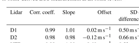
Table 4.Comparison of the instantaneous lidar LOS measurement to sonic-derived LOS measurement at all sonic levels.
Lidar Corr. coeff. Slope Offset SD of differences
D1 0.99 1.01 0.02 m s−1 0.50 m s−1 D2 0.98 0.98 −0.12 m s−1 0.66 m s−1 UTD 0.99 1.00 −0.60 m s−1 0.53 m s−1
3 Determining baseline uncertainty
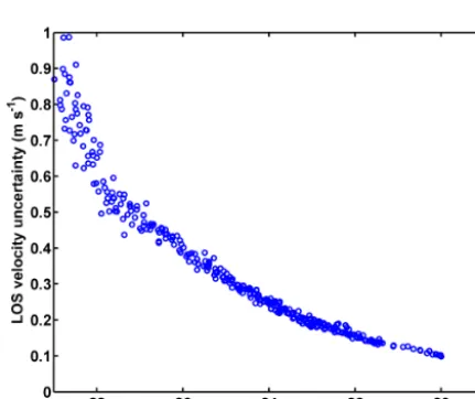
Uncertainties emerge associated with the LOS velocity mea-surements made by the Doppler lidar. These uncertainties can be categorized into (1) random error in the estimation of the velocity and (2) error due to the path integration (range-gating) inherent in pulsed Doppler lidar measurements. The random component of the LOS velocity estimate, for D1, found by linearly fitting the autocovariance of the LOS ve-locity from lags 1 through 4 and extrapolating to zeroth lag (Lenschow et al., 2000) is shown in Fig. 6. Similar values were estimated for all three 200S lidars (D1, D2 and UTD) and the error was a function of signal-to-noise ratio only.
Figure 4.Scans performed by each of the scanning Doppler lidars to produce a 3-D volume of horizontal wind field.(a)Representation of the PPI sector scans performed by each lidar.(b)Grid points that have LOS velocities from at least two lidars and the colors indicate difference in azimuth between their respective look directions.
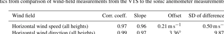
Table 5.Statistics from comparison of wind-field measurements from the VTS to the sonic anemometer measurements.
Wind field Corr. coeff. Slope Offset SD of differences
Figure 5.OI retrieval of the horizontal wind field on a PPI scan performed by D1 on 25 April, 16:52 UTC.(a)LOS velocity field (in m s−1) measured by D1.(b)Horizontal wind field retrieved using the OI technique. The colors indicate magnitude of horizontal wind speed (in m s−1) and wind direction is indicated by arrows.
Figure 6.Estimate of the standard deviation of random error as a function of signal-to-noise ratio estimated using Lenschow et al. (2000).
measurements was compared to the power spectrum of the sonic-derived LOS measurements. Data from a 3-day period where the 200S lidars (D1, D2 and UTD) were performing hour long stares at each sonic anemometer level were used. The spectra of the lidar LOS velocity measurements from the various hour long stares at each sonic anemometer level were averaged and compared to correspondingly averaged sonic-derived LOS measurements (see Fig. 7a). As seen in Fig. 7a, the spectra from the lidar LOS measurements (blue line) flattens out for frequencies higher than∼0.25 Hz, in-dicating that the variations due to random noise dominate. Once the variations due to random noise are subtracted from the spectra, the underprediction of the variability due to the pulse averaging is clearly visible and can be estimated (see Fig. 7b). This underestimation of the variability is defined as the square root of the difference between the spectra of the
sonic anemometer and the lidar measurement and is found to be 0.23 m s−1. The underestimation of the variability can be interpreted as a smoothing of the lidar measurements and hence adds to the differences between the lidar and sonic anemometer wind measurements.
Finally, the total difference between the 1 Hz lidar-measured LOS velocity and the 1 Hz sonic-derived LOS ve-locity measurements, as estimated from direct comparison is presented in Table 4 (Lundquist et al., 2016b). This differ-ence is slightly larger than the combined uncertainties from random noise and pulse averaging. This difference in the un-certainty estimates could be due to some factors that are as yet unaccounted or due to improper estimate of the uncer-tainties due to random noise and pulse averaging. The un-certainty of the LOS measurement by the lidar (when com-pared to the sonic anemometer) allows evaluating the various measurement techniques in terms of additional uncertainty added to this baseline value. The offset in the LOS velocity of the UTD lidar was found to be due to improper calibration of the pulse-length-dependent frequency offset (Lundquist et al., 2016a). This was characterized using independent mea-surements and was found to be constant throughout the XPIA campaign. Therefore, in all measurements presented in this paper, this static offset has been subtracted from the UTD lidar LOS velocity.
4 Validation of wind-field measurements
Figure 7.Comparison of the spectra of LOS data measured by the lidar and the LOS derived from the sonic anemometer measurements. The solid black line indicates the energy cascade following the−5/3 Kolmogorov energy spectrum.(a)Comparison of the spectra showing the noise floor of the Doppler lidar measurements (dotted black line).(b)Comparison of the spectra after subtracting the noise from the lidar spectra. The underprediction of the variability due to the pulse averaging can be seen clearly and found to be 0.23 m s−1.
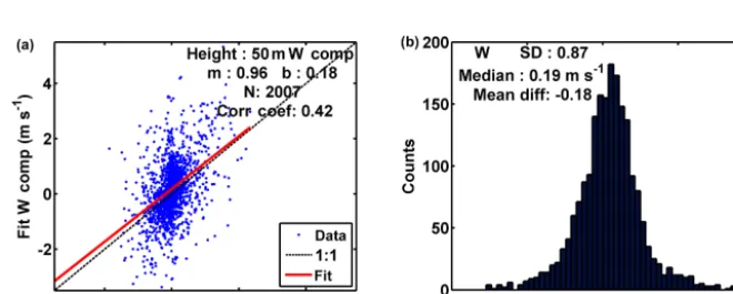
Figure 8.Comparison of the vertical velocity measurements from VTS at the 50 m level with the sonic anemometer measurements.
4.1 Virtual tower stares
The 3-D wind was measured using the VTS technique by tak-ing 5 s of LOS velocity data from the three 200S lidars which overlapped in time and space (as defined by the common vol-ume) and least-squares fitted to Eq. (1) to derive the 3-D wind field. The comparisons of the 3-D wind field as measured by the VTS technique to 5 s averaged sonic anemometer mea-surements are shown in Table 5. These meamea-surements agree with a high correlation coefficient (0.97 and 0.99 for wind speed and direction, respectively) and low standard devia-tion of the differences (0.51 m s−1and 10.16◦for horizontal wind speed and horizontal wind direction, respectively) be-tween the sonic anemometer and the VTS measurements. In addition, the vertical velocity measurements also show a rea-sonably good correlation coefficient (0.86) and low standard deviation of differences (0.5 m s−1). Note that in the verti-cal velocity comparisons, only measurements at and above the 150 m sonic are compared. This is due to the fact that at
the lower sonic levels, the elevation angles in the VTS scans were quite low and as a result the component we are trying to estimate is perpendicular to the lidar look direction, resulting in a noisy vertical velocity retrieval. The velocity retrievals at the 50 m level from the VTS scans are shown in Fig. 8. As can be observed from Fig. 8, there is no skill in the vertical velocity retrievals at low elevation angles.
4.2 Coordinated sparse sampling
ex-Figure 9.Comparison of the(a, b)wind speed,(c, d)wind direction and(e, f)vertical velocity measurements from the SCB technique with the measurements made by the sonic anemometer.
plained in the previous section. The main difference between the VTS measurement strategy and the SCB strategy is the amount of time buffer allowed to make overlapping LOS measurements. In the VTS strategy, each lidar performed a stare scan for 25 s at each measurement location, while it was 5 s for the SCB strategy. Therefore, there was less time to ensure measurement overlap in the SCB strategy and it is expected to have slightly higher uncertainty in wind-field measurement.
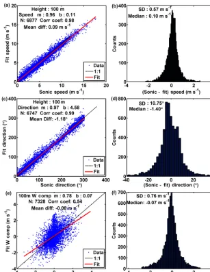
4.3 Uncoordinated virtual tower technique (UVT) The measurements made from the UVT technique were com-pared to the 15 s averaged sonic anemometer measurements at all six levels of the BAO tower. Figure 10 shows that the measurements from the UVT technique have good agreement with the sonic anemometer measurements with correlation
Figure 10.Comparison of the(a, b)wind speed,(c, d)wind direction and(e, f)vertical velocity measurements from the uncoordinated virtual tower technique with the measurements made by the sonic anemometer.
Figure 12.Comparison of the(a, b)wind speed and ((c, d)wind direction measurements from the uncoordinated volume scan technique with the measurements made by the sonic anemometer.
4.4 Uncoordinated volume scan
The uncoordinated volume scan strategy further relaxes the requirement for each lidar to make simultaneous LOS mea-surements at each measurement location and instead uses all LOS velocity measurements from all Doppler lidars that fall within the grid volume and are within a given time window (in this case 5 min) to make a wind-field measure-ment. Comparison of the uncoordinated volume scan mea-surements with 5 min averaged sonic anemometer measure-ments (at three levels from 50 to 150 m) shows good correla-tion coefficients of 0.95 and 0.99 for wind speed and direc-tion, respectively (see Fig. 12).
The standard deviation of the differences between the un-coordinated volume scan measurements and sonic anemome-ter measurements (0.78 m s−1for horizontal wind speed and 13.52◦for horizontal wind direction) is higher compared to the differences reported for the coordinated measurement techniques. The higher uncertainties could be due to non-stationarity of the winds over the measurement accumula-tion period, the effect of which is expected to be much larger compared to the case of UVT technique due to the longer measurement accumulation period. Another factor (which is related to the non-stationarity of the wind) is the less rep-resentative LOS velocity statistics, which is due to the fact that since each lidar does not spend enough time measuring within each grid cell. As a result, the mean of the LOS veloc-ity measurements from each lidar is not representative of the mean velocity over which the wind retrieval is made. 4.5 Single-Doppler OI technique
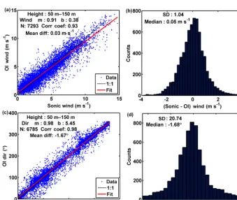
The OI technique allows retrieval of 2-D wind field over conical scans without applying the assumption of horizon-tal homogeneity of the wind. The OI technique was applied to the sector scans performed by each lidar in the uncoor-dinated volume scan technique. Each sector scan took 30 s to complete, and hence the OI retrieval is compared to 30 s averaged sonic anemometer measurement shown in Fig. 13. The retrievals from the OI technique agree with the sonic anemometer measurements quite well with correlation co-efficients of 0.93 and 0.98 for wind speed and wind direc-tion, respectively. The standard deviation of the differences (1.04 m s−1 for horizontal wind speed and 20.74◦ for hori-zontal wind direction) are higher, compared to the uncoordi-nated volume scan technique.
5 Discussion of results
The precision of the wind measurement (defined as the stan-dard deviation of the differences between the Doppler mea-surement and the sonic anemometer meamea-surement) obtained from the various Doppler lidar techniques can now be com-pared. The measurement precision reported for each of the techniques is related to the time it takes to perform one
mea-surement and hence the time average used to evaluate the technique. This method is chosen so that the inherent trade-off between spatial coverage and temporal resolution is clear. Figure 14 shows the comparison of the uncertainties for the LOS velocity as well as the estimates of the horizon-tal wind speed and direction from the various measurement techniques. As seen from Fig. 14, the uncertainty in the LOS velocity (from comparison with sonic anemometer) is 0.5 m s−1. It is observed that with an averaging time of 5 s for the VTS method, the uncertainty does not increase compared to the sonic-derived LOS velocity uncertainty. The most probable reason the precision of the VTS technique is found to be the highest (compared to other velocity retrieval tech-niques presented here) is due to the fact that the three 200S lidars made simultaneous measurements within the common volume and thus relying less heavily on the assumption of stationarity of the atmosphere or spatial homogeneity. In-creasing the measurement complexity and spatial coverage either through faster scanning or relaxing the requirement of temporal coordination increases the measurement uncer-tainty as well. The reasons for this could be two-fold. First, since the measurements are not temporally synchronized, the non-stationarity of the atmosphere increases the uncertainty in the measurement; secondly, due to faster scanning, there are fewer LOS velocity measurements within each measure-ment volume resulting in nonrepresentative LOS velocity statistics that result in a poorer estimation of the mean wind. The latter issue is expected to be less dominant in simpler un-coordinated strategies such as the UVT and more dominant in strategies involving covering large spatial extents such as the uncoordinated volume scan. While the single-Doppler OI does not require complex scanning technique, it requires cer-tain assumptions as part of the retrieval process (Choukulkar et al., 2012) and hence increases the measurement uncer-tainty.
Figure 14.Measurement uncertainties for(a)horizontal wind speed and(b)horizontal wind direction estimated for the different measurement strategies investigated.
Effect of stability
The precision of wind measurements is also evaluated in var-ious stability conditions. The stability is defined using hourly averaged virtual potential temperature gradient between the 50 m level and the 300 m level using both the tower measure-ments and radiometer measuremeasure-ments (Bianco et al., 2016).
Conditions were determined to be stable for positive gradient of the virtual potential temperature and unstable for a nega-tive gradient of the virtual potential temperature.
Figure 15.Measurement uncertainty as a function of stability for(a)horizontal wind speed and(b)horizontal wind direction.
that unstable conditions show higher variability than stable conditions, which might lead to higher level of uncertainty. However, no consistent pattern emerges for the effect of sta-bility on wind direction uncertainty. This might be due to the fact that all the stable conditions examined here were accom-panied by low wind conditions, which usually leads to higher variability in wind direction, while the unstable conditions had higher wind speeds. As a result, the wind direction un-certainty during stable conditions is found to be higher. It is
clear from Fig. 15 that stability and spatial variability do have a significant impact on the measurement uncertainty.
6 Conclusions
Doppler lidars is understanding the inherent uncertainties as-sociated with the corresponding measurement technique. In this paper, the uncertainties associated with Doppler lidar measurements were quantified starting with the uncertainties due to random noise and pulse averaging to uncertainties as-sociated with single- and multi-Doppler measurement tech-niques.
It was found that as complexity of the measurement tech-nique and/or the spatial coverage of measurements made creased, the uncertainty in the wind measurement also in-creased. For multi-Doppler measurements, the magnitude of uncertainty was associated with ability to make coordi-nated measurements. Measurements made using accurate co-ordinated scanning resulted in lower uncertainties compared to measurements from temporally uncoordinated scanning. This result is expected due to the non-stationarity of the at-mosphere, sampling error in LOS velocity statistics and pres-ence of spatial variability in the wind field. As a result, the coordinated VTS techniques resulted in the lowest measument uncertainty, while the single-Doppler OI technique re-sulted in the highest measurement uncertainty (compared to multi-Doppler techniques), but also had the largest spatial coverage at high update rates and is less expensive as a re-sult of requiring only one lidar.
The results illustrate the tradeoff between making highly precise measurements at one location versus accepting a lower precision but covering larger spatial extents. Although the magnitude of the uncertainties for the various measure-ment techniques presented in this paper might not be repro-ducible at other locations and under different wind condi-tions, the trends observed should be similar. This quantifica-tion of the uncertainty as a funcquantifica-tion of measurement tech-nique allows proper selection of measurement strategy given the goals of the experiment and interpretation of the mea-surements made using those techniques.
7 Data availability
The data from all the instruments deployed during the XPIA field campaign are now available at DOE’s Data Access Portal (DAP) located at https://a2e.pnnl.gov/data (Lundquist et al., 2016c). Access to the general pub-lic has been open since 1 April 2016. In order to ac-cess the data, users need to create an account on the website given above. For further inquiries please con-tact either Julie Lundquist ([email protected]) or James Wilczak ([email protected]).
Acknowledgement. The authors acknowledge the funding for this work provided by the US Department of Energy, Office of Energy Efficiency and Renewable Energy and by NOAA’s Earth System Research Laboratory. The authors also acknowledge contributions of numerous individuals and organization who assisted with the field deployment including Bruce Bartram,
Duane Hazen, Tom Ayers, Jesse Leach, Paul Johnston, Left-hand Water District, Erie High School and the St. Vrain School District. We also express our appreciation to NOAA/Earth Systems Research Laboratory/Physical Sciences Division for supporting the instrumentation at the BAO facility. We express appreciation to the National Science Foundation for supporting the CABL deployments (https://www.eol.ucar.edu/field_projects/cabl) of the tower instrumentation. NREL is a national laboratory of the US De-partment of Energy, Office of Energy Efficiency and Renewable Energy, operated by the Alliance for Sustainable Energy, LLC.
Edited by: A. Clifton
Reviewed by: two anonymous referees
References
Banta, R. M., Pichugina, Y. L., Brewer, W. A., Lundquist, J. K., Kelley, N. D., Sandberg, S. P., Alvarez II, R. J., Hard-esty, R. M., and Weickmann, A. M.: 3D Volumetric Analysis of Wind Turbine Wake Properties in the Atmosphere Using High-Resolution Doppler Lidar, J. Atmos. Ocean. Tech., 32, 904–914, doi:10.1175/JTECH-D-14-00078.1, 2015.
Barlow, J. F., Dunbar, T. M., Nemitz, E. G., Wood, C. R., Gallagher, M. W., Davies, F., O’Connor, E., and Harrison, R. M.: Boundary layer dynamics over London, UK, as observed using Doppler li-dar during REPARTEE-II, Atmos. Chem. Phys., 11, 2111–2125, doi:10.5194/acp-11-2111-2011, 2011.
Berg, J., Vasiljevíc, N., Kelly, M., Lea, G., and Courtney, M.: Ad-dressing Spatial Variability of Surface-Layer Wind with Long-Range WindScanners, J. Atmos. Ocean. Tech., 32, 518–527, doi:10.1175/JTECH-D-14-00123.1, 2015.
Bianco, L., Friedrich, K., Wilczak, J., Hazen, D., Wolfe, D., Del-gado, R., Oncley, S., and Lundquist, J. K.: Assessing the accu-racy of microwave radiometers and radio acoustic sounding sys-tems for wind energy applications, Atmos. Meas. Tech. Discuss., doi:10.5194/amt-2016-321, in review, 2016.
Bingöl, F., Mann, J., and Foussekis, D.: Conically scanning lidar error in complex terrain, Meteorol. Z., 18, 189–195, doi:10.1127/0941-2948/2009/0368, 2009.
Browning, K. A. and Wexler, R.: The determination of kinematic properties of a wind field using Doppler radar, J. Appl. Meteorol., 7, 105–113, 1968.
Calhoun, R., Heap, R., Princevac, M., Newsom, R., Fernando, H., and Ligon, D.: Virtual towers using coherent Doppler lidar dur-ing the Joint Urban 2003 dispersion experiment, J. Appl. Meteo-rol. Clim., 45, 1116–1126, 2006.
Chan, P. W. and Shao, A. M.: Depiction of complex airflow near Hong Kong International Airport using a Doppler LIDAR with a two-dimensional wind retrieval technique, Meteorol. Z., 16, 491– 504, 2007.
Cherukuru, N. W., Calhoun, R., Lehner, M., Hoch, S. W., and Whiteman, C. D.: Instrument configuration for dual-Doppler li-dar coplanar scans: METCRAX II, J. Appl. Remote Sens., 9, 096090, doi:10.1117/1.JRS.9.096090, 2015.
Choukulkar, A., Calhoun, R., Billings, B., and Doyle, J. D.: A mod-ified optimal interpolation technique for vector retrieval for co-herent Doppler lidar, Geosci. Remote Sens. Lett., 9, 1132–1136, 2012.
Collier, C. G., Davies, F., Bozier, K. E., Holt, A. R., Middleton, D. R., Pearson, G. N., Siemen, S., Willetts, D. V., Upton, G. J. G., and Young, R. I.: Dual-Doppler Lidar Measurements for Im-proving Dispersion Models, B. Am. Meteor. Soc., 86, 825–838, doi:10.1175/BAMS-86-6-825, 2005.
Damian, T., Wieser, A., Träumner, K., Corsmeier, U., and Kottmeier, C.: Nocturnal Low-level Jet Evolution in a Broad Val-ley Observed by Dual Doppler Lidar, Meteorol. Z., 305–313, 2014.
Drechsel, S., Mayr, G. J., Chong, M., Weissmann, M., Dörnbrack, A., and Calhoun, R.: Three-Dimensional Wind Retrieval: Ap-plication of MUSCAT to Dual-Doppler Lidar, J. Atmos. Ocean. Tech., 26, 635–646, doi:10.1175/2008JTECHA1115.1, 2009. Fernando, H. J. S., Pardyjak, E. R., Di Sabatino, S., Chow, F. K.,
De Wekker, S. F. J., Hoch, S. W., Hacker, J., Pace, J. C., Pratt, T., Pu, Z., Steenburgh, W. J., Whiteman, C. D., Wang, Y., Zajic, D., Balsley, B., Dimitrova, R., Emmitt, G. D., Higgins, C. W., Hunt, J. C. R., Knievel, J. C., Lawrence, D., Liu, Y., Nadeau, D. F., Kit, E., Blomquist, B. W., Conry, P., Coppersmith, R. S., Creegan, E., Felton, M., Grachev, A., Gunawardena, N., Hang, C., Hocut, C. M., Huynh, G., Jeglum, M. E., Jensen, D., Kulandaivelu, V., Lehner, M., Leo, L. S., Liberzon, D., Massey, J. D., McEner-ney, K., Pal, S., Price, T., Sghiatti, M., Silver, Z., Thompson, M., Zhang, H., and Zsedrovits, T.: The MATERHORN: Unraveling the Intricacies of Mountain Weather, B. Am. Meteor. Soc., 96, 1945–1967, doi:10.1175/BAMS-D-13-00131.1, 2015.
Fuertes, F. C., Iungo, G. V., and Porté-Agel, F.: 3D Turbulence Mea-surements Using Three Synchronous Wind Lidars: Validation against Sonic Anemometry, J. Atmos. Ocean. Tech., 31, 1549– 1556, doi:10.1175/JTECH-D-13-00206.1, 2014.
Gunter, W. S., Schroeder, J. L., and Hirth, B. D.: Validation of Dual-Doppler Wind Profiles with in situ Anemometry, J. Atmos. Ocean. Tech., 32, 943–960, doi:10.1175/JTECH-D-14-00181.1, 2015.
Hill, M., Calhoun, R., Fernando, H. J. S., Wieser, A., Dörnbrack, A., Weissmann, M., Mayr, G., and Newsom, R.: Coplanar Doppler lidar retrieval of rotors from T-REX, J. Atmos. Sci., 67, 713–729, 2010.
Kaimal, J. C. and Gaynor, J. E.: The Boulder Atmospheric Observa-tory, J. Clim. Appl. Meteorol., 22, 863–880, doi:10.1175/1520-0450(1983)022<0863:TBAO>2.0.CO;2, 1983.
Käsler, Y., Rahm, S., Simmet, R., and Kühn, M.: Wake Measure-ments of a Multi-MW Wind Turbine with Coherent Long-Range Pulsed Doppler Wind Lidar, J. Atmos. Ocean. Tech., 27, 1529– 1532, doi:10.1175/2010JTECHA1483.1, 2010.
Klein, P., Bonin, T. A., Newman, J. F., Turner, D. D., Chil-son, P. B., Wainwright, C. E., Blumberg, W. G., Mishra, S., Carney, M., Jacobsen, E. P., Wharton, S., and Newsom, R. K.: LABLE: A Multi-Institutional, Student-Led, Atmospheric Boundary Layer Experiment, B. Am. Meteor. Soc., 96, 1743– 1764, doi:10.1175/BAMS-D-13-00267.1, 2015.
Krishnamurthy, R., Choukulkar, A., Calhoun, R., Fine, J., Oliver, A., and Barr, K. S.: Coherent Doppler lidar for wind farm char-acterization, Wind Energy, 16, 189–206, 2013.
Lenschow, D. H., Wulfmeyer, V., and Senff, C.: Measuring second-through fourth-order moments in noisy data, J. Atmos. Ocean. Tech., 17, 1330–1347, 2000.
Lundquist, J. K., Churchfield, M. J., Lee, S., and Clifton, A.: Quan-tifying error of lidar and sodar Doppler beam swinging measure-ments of wind turbine wakes using computational fluid dynam-ics, Atmos. Meas. Tech., 8, 907–920, doi:10.5194/amt-8-907-2015, 2015.
Lundquist, J. K., Wilczak, J. M., Ashton, R., Bianco, L., Brewer, W. A., Choukulkar, A., Clifton, A., Debnath, M., Delgado, R., Friedrich, K., Gunter, S., Hamidi, A., Iungo, G. V., Kaushik, A., Kosovi´c, B., Langan, P., Lass, A., Lavin, E., Lee, J. C.-Y., McCaffrey, K. L., Newsom, R. K., Noone, D. C., Oncley, S. P., Quelet, P. T., Sandberg, S. P., Schroeder, J. L., Shaw, W. J., Spar-ling, L., St. Martin, C., St. Pe, A., Strobach, E., Tay, K., Vander-wende, B. J., Weickmann, A., Wolfe, D., and Worsnop, R.: As-sessing state-of-the-art capabilities for probing the atmospheric boundary layer: the XPIA field campaign, B. Am. Meteor. Soc., doi:10.1175/BAMS-D-15-00151.1, online first, 2016a.
Lundquist, J. K., Wilczak, J. M., Ashton, R., Bianco, L., Brewer, W. A., Choukulkar, A., Clifton, A., Debnath, M., Delgado, R., Friedrich, K., Gunter, S., Hamidi, A., Iungo, G. V., Kaushik, A., Kosovi´c, B., Langan, P., Lass, A., Lavin, E., Lee, J. C.-Y., McCaffrey, K. L., Newsom, R. K., Noone, D. C., Oncley, S. P., Quelet, P. T., Sandberg, S. P., Schroeder, J. L., Shaw, W. J., Spar-ling, L., St. Martin, C., St. Pe, A., Strobach, E., Tay, K., Vander-wende, B. J., Weickmann, A., Wolfe, D., and Worsnop, R.: As-sessing state-of-the-art capabilities for probing the atmospheric boundary layer: the XPIA field campaign, National Renewable Energy Laboratory (NREL), Golden, CO, 2016b.
Lundquist, J. K., Wilczak, J. M., Ashton, R., Bianco, L., Brewer, W. A., Choukulkar, A., Clifton, A., Debnath, M., Delgado, R., Friedrich, K., Gunter, S., Hamidi, A., Iungo, G. V., Kaushik, A., Kosovi´c, B., Langan, P., Lass, A., Lavin, E., Lee, J. C.-Y., McCaffrey, K. L., Newsom, R. K., Noone, D. C., Oncley, S. P., Quelet, P. T., Sandberg, S. P., Schroeder, J. L., Shaw, W. J., Spar-ling, L., St. Martin, C., St. Pe, A., Strobach, E., Tay, K., Vander-wende, B. J., Weickmann, A., Wolfe, D., and Worsnop, R.: XPIA, Pacific Northwest National Laboratory, Department of Energy, available at: https://a2e.pnnl.gov/data (last access: 18 January 2017), 2016c.
Mann, J., Cariou, J.-P., Courtney, M. S., Parmentier, R., Mikkelsen, T., Wagner, R., Lindelöw, P., Sjöholm, M., and Enevoldsen, K.: Comparison of 3D turbulence measurements using three staring wind lidars and a sonic anemometer, Meteorol. Z., 18, 135–140, doi:10.1127/0941-2948/2009/0370, 2009.
McCaffrey, K., Quelet, P., Choukulkar, A., Wilczak, J. M., Wolfe, D. E., Oncley, S., Brewer, A., Debnath, M., Ashton, R., Iungo, G. V., and Lundquist, J. K.: Identification of Tower Wake Dis-tortions Using Sonic Anemometer and Lidar Measurements, At-mos. Meas. Tech. Discuss., doi:10.5194/amt-2016-179, in re-view, 2016.
Mikkelsen, T.: Lidar-based research and innovation at DTU wind energy–a review, in Journal of Physics: Conference Series, vol. 524, p. 012007, IOP Publishing, available at: http://iopscience.iop.org/article/10.1088/1742-6596/524/1/ 012007/meta (last access: 22 August 2016), 2014.
doppler lidars, in IOP Conference Series: Earth and Environmen-tal Science, 1, U148–U156, Institute of Physics Publishing Ltd., 2008.
Newman, J. F., Bonin, T. A., Klein, P. M., Wharton, S., and New-som, R. K.: Testing and validation of multi-lidar scanning strate-gies for wind energy applications, Wind Energy, 19, 2239–2254, doi:10.1002/we.1978, 2016.
Newsom, R., Calhoun, R., Ligon, D., and Allwine, J.: Linearly organized turbulence structures observed over a suburban area by dual-Doppler lidar, Bound.-Layer Meteorol., 127, 111–130, 2008.
Newsom, R. K., Berg, L. K., Shaw, W. J., and Fischer, M. L.: Turbine-scale wind field measurements using dual-Doppler lidar, Wind Energy, 18, 219–235, doi:10.1002/we.1691, 2015. Simley, E., Angelou, N., Mikkelsen, T., Sjöholm, M., Mann,
J., and Pao, L. Y.: Characterization of wind velocities in the upstream induction zone of a wind turbine using scanning continuous-wave lidars, J. Renew. Sustain. Energy, 8, 013301, doi:10.1063/1.4940025, 2016.
Stawiarski, C., Träumner, K., Knigge, C., and Calhoun, R.: Scopes and challenges of dual-Doppler lidar wind measurements – an error analysis, J. Atmos. Ocean. Tech., 30, 2044–2062, 2013. Strauch, R. G., Merritt, D. A., Moran, K. P., Earnshaw, K.
B., and De Kamp, D. V.: The Colorado Wind-Profiling Net-work, J. Atmos. Ocean. Tech., 1, 37–49, doi:10.1175/1520-0426(1984)001<0037:TCWPN>2.0.CO;2, 1984.
Träumner, K., Damian, T., Stawiarski, C., and Wieser, A.: Turbu-lent structures and coherence in the atmospheric surface layer, Bound.-Layer Meteorol., 154, 1–25, 2015.
Vanderwende, B. J., Lundquist, J. K., Rhodes, M. E., Takle, E. S., and Irvin, S. L.: Observing and simulating the summertime low-level jet in central Iowa, available at: http://journals.ametsoc.org/ doi/abs/10.1175/MWR-D-14-00325.1 (last access: 24 October 2015), Mon. Weather Rev., 2015.
Vasiljevi´c, N., Lea, G., Courtney, M., Cariou, J.-P., Mann, J., and Mikkelsen, T.: Long-Range WindScanner System, Remote Sens., 8, 1–24, doi:10.3390/rs8110896, 2016.
Vollmer, L., van Dooren, M., Trabucchi, D., Schneemann, J., Stein-feld, G., Witha, B., Trujillo, J., and Kühn, M.: First comparison of LES of an offshore wind turbine wake with dual-Doppler lidar measurements in a German offshore wind farm, J. Phys. Conf. Ser., 625, 012001, doi:10.1088/1742-6596/625/1/012001, 2015. Waldteufel, P. and Corbin, H.: On the analysis of single-Doppler
radar data, J. Appl. Meteorol., 18, 532–542, 1979.
Wang, H., Barthelmie, R. J., Clifton, A., and Pryor, S. C.: Wind Measurements from Arc Scans with Doppler Wind Lidar, J. At-mos. Ocean. Tech., 32, 2024–2040, doi:10.1175/JTECH-D-14-00059.1, 2015.