Ocean Sci., 6, 933–947, 2010 www.ocean-sci.net/6/933/2010/ doi:10.5194/os-6-933-2010
© Author(s) 2010. CC Attribution 3.0 License.
Ocean Science
Spatio-Temporal Complexity analysis of the Sea Surface
Temperature in the Philippines
Z. T. Botin1, L. T. David2, R. C. H. del Rosario1,*, and L. Parrott3
1Institute of Mathematics, University of the Philippines Diliman, 1101 Quezon City, Philippines 2Marine Science Institute, University of the Philippines Diliman, 1101 Quezon City, Philippines
3Departement de G´eographie, Universit´e de Montr´eal, C.P. 6128 succursale centre-ville, Montr´eal, QC H3C 3JY, Canada *now at: Genome Institute of Singapore, 60 Biopolis Street, #02-01 Genome, Singapore
Received: 25 October 2009 – Published in Ocean Sci. Discuss.: 26 November 2009 Revised: 21 October 2010 – Accepted: 29 October 2010 – Published: 9 November 2010
Abstract. A spatio-temporal complexity (STC) measure which has been previously used to analyze data from terres-trial ecosystems is employed to analyse 21 years of remotely sensed sea-surface temperature (SST) data from the Philip-pines. STC on the Philippine wide SST showed the mon-soonal variability of the Philippine waters. STC is correlated with the SST mean (R2≈0.7), and inversely correlated with the SST standard deviation (R2≈0.9). Both STC and SST are highest during the middle of the year, which coincides with the Southwest Monsoon, but with the STC values be-ing higher towards the end of the monsoon until the start of the inter-monsoon. In order to determine if STC has the po-tential to define limits of bio-regions, the spatial domain was subsequently divided into six thermal regions computed via clustering of temperature means. STC and EOF of the STC values were computed for each thermal region. Our STC analysis of the SST data, and comparisons with SST values suggest that the STC measure may be useful for character-ising environmental heterogeneity over space and time for many long-term remotely sensed data.
1 Introduction
Temperature is a controlling factor in ocean systems. Anomalies in sea surface temperature (SST) have a wide range of effects on marine ecosystems including the decline in reef fish populations (Pratchett et al., 2006) and coral
dis-Correspondence to: R. C. H. del Rosario
ease outbreaks (Bruno et al., 2007). In the early 1990s, links between SST and coral bleaching were proposed (Lesser et al., 1990; Glynn and D’Croz, 1990). Strong et al. (1996) subsequently successfully identified suspected areas of coral reef bleaching using satellite derived SST. Recently, Pe˜naflor et al. (2009) focused on the SST of the Coral Triangle (which spans eastern Indonesia, parts of Malaysia, the Philippines, Papua New Guinea, Timor Leste and the Solomon Islands) and highlighted the importance of investigating how SST has changed through space and time within this region.
Here, we explore the hypothesis that the spatio-temporal complexity of the SST signal can be linked to physical pro-cesses such as prevailing winds and weather systems and our objective is to characterize these dynamics. In particular, we assess the ability of a recently developed measure of spatio-temporal complexity (STC) to provide additional informa-tion from the SST data. STC is a relatively new measure whose applications to remotely sensed data in the ocean sci-ences have yet to be demonstrated. If sufficiently sensitive, such a measure could ultimately serve as an indicator of im-pending change in the dynamics of SST, which might help to detect the onset of coral bleaching or other regime shifts in the marine ecosystem.
to disorder. By mixing the ocean surface, we would ex-pect the prevailing weather systems to have an effect on this dynamics, creating seasons during which the SST is more uniform across the Philippine region (ordered), patchy (com-plex) or random (disordered). The measure we use is based on entropy measures arising from information theory. En-tropy measures are standard tools for measuring complexity and have been widely used in ecology to measure species di-versity (Nsakanda et al., 2007). Shannon entropy was first used to measure species diversity in MacArthur (1955) and although it is one of the most popular methods to measure the structural complexity of an ecological system, it is not able to measure the complexity of the system’s dynamics (Parrott, 2005). Other information-based measures (e.g., mean infor-mation gain, effective complexity and fluctuation complex-ity) have been applied to the analysis of temporal data (time series) or to spatial data but rarely to both types of data (An-drienko et al., 2000; Wackerbauer et al., 1994; Parrott et al., 2008; Shalizi and Shalizi, 2003).
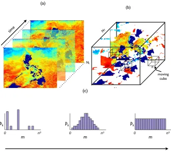
It is important to capture both space and time in complex-ity measures and Parrott (2005) and Parrott et al. (2008) in-troduced STC for this purpose (Fig. 1). It was applied to simulated vegetation data to explore its potential in charac-terising ecological spatio-temporal dynamics (Parrott, 2005) and was successfully used to analyze repeat photography data for a temperate forest in Parrott et al. (2008). STC is based on Shannon entropy and is able to incorporate the three dimensional nature of space-time fluctuations. It can be applied to spatio-temporal data sets wherein the state of a two-dimensional spatial mosaic has been recorded at regu-lar time intervals and it can distinguish between ordered and disordered, complex or patchy spatio-temporal distributions (Parrott et al., 2008). It is also able to detect spatio-temporal patterns such as space-time cycles (Parrott, 2005).
In this paper, we apply the STC algorithm on the 4 km res-olution SST data to study the dynamics of Philippine SST both in space and in time. We investigate how STC performs in distinguishing the years affected by ENSO events, and in distinguishing regions subject to different oceanographic conditions. To identify these regions, K-means clustering was used and the STC of each region was calculated to deter-mine how well the measure could detect changes over time and space. To aid in analyzing the composite STC plots of the Philippine region and of each thermal region, empirical orthogonal functions (EOF) were employed on the STC val-ues.
2 Methods 2.1 SST data
SST data are from 1985–2005 night-time observations of the Advanced Very High Resolution Radiometer (AVHRR) on board the Polar Orbiting Environmental Satellites (POES)
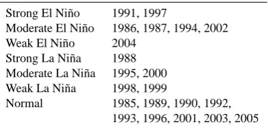
Table 1. ENSO classification from Golden Gate Weather Services.
Strong El Ni˜no 1991, 1997
Moderate El Ni˜no 1986, 1987, 1994, 2002 Weak El Ni˜no 2004
Strong La Ni˜na 1988 Moderate La Ni˜na 1995, 2000 Weak La Ni˜na 1998, 1999
Normal 1985, 1989, 1990, 1992, 1993, 1996, 2001, 2003, 2005
of the National Oceanic and Atmospheric Administra-tion (NOAA). The AVHRR-SST products are twice-weekly datasets and we used its processed form from the AVHRR Pathfinder Project of the National Oceanographic Data Cen-ter (NODC) and the University of Miami’s Rosenstiel School of Marine and Atmospheric Science (see National Oceano-graphic Data Center (2008)). This 4 km resolution SST data was used for the analysis and has a temporal resolution of once a week. The Philippine data was taken from the global data at location 114 to 130 longitude and 4 to 21.5 lati-tude. The resulting spatial dimension of the SST matrix is 399×365 pixels, out of which the Philippine land mass occupies about 10%, and its temporal dimension is 1092 (52 weeks×21 years).
2.2 Classification of ENSO years
We classified all years between 1985 and 2005 as either El Ni˜no, La Ni˜na or normal according to the Oceanic Ni˜no-based list at “El Ni˜no and La Ni˜na Years and Intensities” (Golden Gate Weather Services, 2010). The classification is given in Table 1.
2.3 Measuring Spatio-Temporal complexity
Z. T. Botin et al.: Spatio-Temporal Complexity analysis of Philippine SST 935
time
NW
moving cube NT
NL
n
(a) (b)
pk pk
pk
0 n3 0 n3 0 n3
(c)
Spatiotemporal complexity, STC
m m m
time
NW
moving cube
NT
NL
n
(a) (b)
pk pk
pk
0 n3 0 n3 0 n3
(c)
Spatiotemporal complexity, STC
m m m
time
NW
moving cube NT
NL
n
(a) (b)
pk pk
pk
0 n3 0 n3 0 n3
(c)
Spatiotemporal complexity, STC
m m m
Fig. 1. Schematic of the spatio-temporal complexity analysis: (a) The series of raster-based sea surface temperature (SST) images are stacked into a 3-D space-time matrix. (b) A threshold temperature is applied to generate a binary matrix, in which all cells below the threshold have zero values (shown here as empty cells). Ann×n×nmoving cube is placed at successive locations in the space-time matrix like a sliding window. At each location, the number of non-zero entries (m) in the cube is noted. The relative frequency,pk, that each occupancy level,
m, is observed is calculated. (c) Frequency histograms ofpk versusm. A highly uneven histogram (left) is indicative of ordered space-time dynamics and gives a low value of spatio-temporal complexity (STC). A bell-shaped histogram (middle) is indicative of a random distribution of non-zero entries in the space-time matrix and gives an intermediate value of STC. A perfectly even histogram (right) arises when the space-time matrix is populated with patches of all different sizes and shapes and gives a maximal value of STC.
After converting the data to binary, it is stacked into a 3-dimensionalNL×NW×NT matrix, and a “moving cube” is made to traverse the matrix while counting the num-ber of non-zero entries (within the cube) at each position (see Fig. 1). To incorporate the temporal dimension of the data, the dimension, c, of this cube is taken to be at least 2 but much smaller than the dimensions of the data ma-trix (i.e., 2≤nmin(NL,NW,NT)). The total number of possible positions of the cube inside the data matrix is M=(NL−n+1)×(NW−n+1)×(NT−n+1). At each position of the moving cube, the number of non-zero entries (or the occupancy level) is denoted bymi,i=1,...,M, and we tabulate the number of times the occupancy levelmi ap-pears. Specifically, for an occupancy level ofk, we count the number ofmi such thatmi=k and denote this asµk. The relative frequency ofk non-zero entries, denoted bypk, is
given by pk=
µk µ0+µ1+...+µn3
, (1)
and the spatio-temporal complexity of theNL×NW×NT data matrix is given by
STC= −
n3 X
k=0
pk lnpk
ln(n3+1) . (2)
Here we impose that lnpk=0 ifpk=0.
used time slices with thicknesss=3,4,5 (i.e., STC is calcu-lated for data matrices ofNL×NW×s). We used moving cube sizes ofc=3,4,5 wherec≤s. Furthermore, we also considered both non-overlapping and overlapping slices.
It is mathematically proven in Botin (2009) that forc≥2, STC gives the lowest value to a completely ordered 3-D data matrix and that it gives the highest value to a data ma-trix where all occupation levels are observed with equal fre-quencies. The highest value of STC thus corresponds to a spatio-temporal dynamics consisting of many frequent small patches and several large irregular patches that are constantly changing their sizes and locations in space and time. If we consider the patches as three-dimensional “blobs” in space-time, then the frequency distribution of blob volumes for a data matrix having an STC value of 1 follows a power law distribution (Parrott et al., 2008). On the other hand, a data matrix containing large sized and regularly shaped patches of non-zero entries would have high frequencies for fully occupied cubes and empty cubes and low frequencies for non-empty cubes that are not fully occupied. Since this is closer to an ordered case, STC will assign a low value for this kind of data. Furthermore, Parrott (2005) discussed that un-like Shannon entropy which assigns the highest value to ran-domly generated data, STC assigns intermediate values for randomly generated binary 3-D matrices. Thus, according to the classification of complexity measures by Atmanspacher (2007), we can classify STC under the class of measures where complexity is a convex function of randomness.
High STC is thus of interest in a geophysical context, since it is an indication that the space-time dynamics of the vari-able studied has a scale-invariant, fractal structure, as typified by the power law distribution of blob sizes in the space-time matrix. Power-laws have been observed in many time series for physical systems and in spatial data, and fractal structures seem to be ubiquitous across many physical systems (Tur-cotte, 1997). In dynamical systems, the presence of power-law behavior in space or time is a necessary but not sufficient condition for first order phase transitions and self-organized criticality (Bak and Chen, 1991; Goldenfeld, 1992; Reichl, 1998) and it is possible that this extends to spatiotemporal dynamics under regimes of high STC.
2.4 Identification of the thermal regions
To identify thermal regions with distinct temporal and spatial variability, we followed the method in Pe˜naflor et al. (2009). We used the web-based geospatial clustering tool Deluxe In-tegrated System for Clustering Operations (DISCO; Budde-meier et al. (2008); accessible at http://fangorn.colby.edu/ disco-devel). Due to data limitations imposed by DISCO, we obtained the average monthly temperature of each pixel/point of the spatial domain. Input data files for DISCO were pre-pared by arranging each pixel data on one row, with each column containing averaged SST data for a month. Then the K-means algorithm (in DISCO) was employed on the entire
domain and was allowed to search from 5 to 10 clusters. It obtained 6 optimal clusters as determined by the “Minimum Description Length” (MDL). The centroid of each cluster was obtained and a rectangular region was chosen to have a height of around 35 pixels and width of around 50 pixels, which fit within the cluster and which does not overlap pix-els on land. The resulting regions are shown in Fig. 2 and are used in later analyses.
2.5 Empirical Orthogonal Function analysis of the STC The Empirical Orthogonal Functions (EOF) analysis used in oceanography is the same as Principal Component Analy-sis (PCA) and has also been called Proper Orthogonal De-composition (POD) in reduced order modeling (Banks et al., 2002). EOFs provide an efficient method of compressing data (Emery and Thomson, 2001; Banks et al., 2002) and the EOFs represent the uncorrelated modes of variability of the data (Emery and Thomson, 2001).
In EOF analysis, the data is typically from concurrent time-series records gathered by a grid of recording stations. In order to perform EOF analysis on the Philippine-wide STC values, we separate the STC time histories by year, group them into El Ni˜no, La Ni˜na and normal, and con-sider that they were measured concurrently during the same year. Thus for the El Ni˜no group, the different yearly time-histories represent the time histories taken by different recording stations. This alleviates the technical difficulty that the STC measurements were taken at the same location (i.e, the whole Philippines) and that the measurements were not taken in one year but during different years. For each group, we then look for a set of orthogonal predictors or modes whose linear combination could account for the combined variance in all of the observations.
To illustrate its application to Philippine-region analysis of El Ni˜no years, let us denote the yearly STC bySj(ti),j= 1,...,M,i=1,...,N. N denotes the number of STC time-points in each year, whileMis the number of El Ni˜no years. If strong, moderate and weak ENSO years are used, then from Table 1 we haveM=7. Since overlapping time-slices were used in STC calculations, the number of STC data points for the last year (2005) is not equal to the rest of the years. Therefore in the EOF analysis we exclude the values for 2005 which is classified as normal. For each yearj, the mean is subtracted fromSj to obtain the anomaly field, or departure from the climatology field:S˜j=Sj−Sj.
EOF analysis yields M orthogonal basis functions (or modes)φk(x)such that
˜
Sj(t )= M X
k=1
αk(t )φk(xj) , (3)
Z. T. Botin et al.: Spatio-Temporal Complexity analysis of Philippine SST 937
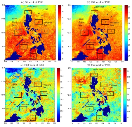
(a) 6th week of 1988 (b) 10th week of 1988
(c) 23rd week of 1988 (d) 33rd week of 1988
Fig. 2. SST during the NE monsoon season (a and b) and SW monsoon (c and d). The arrows indicate the direction of the prevailing winds (not scaled to indicate wind strength). The locations of the six thermal regions are indicated in boxes.
To compute the EOF basis functions and time-dependent amplitudes (also denoted as principal components), theM×
Mcovariance matrixS is created, with elementsSij= ˜SiT· ˜
Sj. The eigenvectorsVkand the corresponding eigenvalueαk ofSare computed. In order to compare the EOF results with the EOF of other ENSO years, we normalized the eigenvec-tors byVk=Vk/(
√
N αk)(Banks et al., 2002). As detailed in Emery and Thomson (2001), the EOF basis functions and time-dependent amplitudes are given respectively by
φk(xj)= [Vk]j,αk(t )= M X
m=1 ˜
Sm(t )[Vk]m. (4)
For the EOF analysis of SST data, denoted also bySj(ti),
the subscriptjis the index of the location of the observation points while the subscriptiis the index of the measurement time-points.
For EOF analysis of the STC of thermal regions, the STC values are grouped according to the thermal regions and thus the analysis is more analogous to the EOF analysis of SST data (since measurements are taken at different locations).N has the same value as in the Philippine region EOF analysis, whileMis the number of years measured in each thermal re-gion – which is the same for all 6 rere-gions. We also performed an EOF analysis of the thermal regions grouped according to ENSO classification.
Perform EOF calculations on STC Analysis
Whole−Country Cluster whole−country
data to obtain thermal region boundaries Thermal Region
STC Analysis
Choose appropriate time−slice and moving cube size and compute the STC
Prepare SST data to be analyzed (ENSO group/region) and stack into a 3−D matrix
Determine threshold and convert the data into binary
EOF Analysis STC Computation STC Computation Data Preparation
of STC
OR
Plot the time−dependent amplitudes Plot time−history
of the EOF modes
selected STC values to be analyzed
Fig. 3. A flowchart of the steps in the analysis of SST data.
3 Results and Discussion
3.1 STC of the whole Philippine region
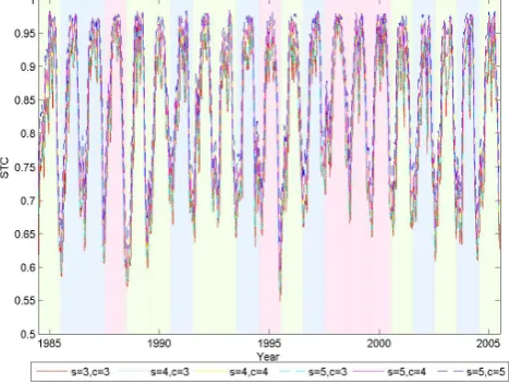
The Philippine region considered in this analysis is shown in Fig. 2. In Fig. 4, we plot the STC of the weekly Philip-pine SST from 1985 to 2005 using overlapping time slices with thicknesss=3,4,5 and moving cube sizesc=3,4,5, wherec≤s. Two consecutive time slices overlap in s−1 time points wheresis the thickness of the time slice, i.e., if theith time slice contains the time pointsTi,Ti+1,...Ti+s−1,
then the next time slice containsTi+1,Ti+2,...Ti+s. A mov-ing average threshold of 5 weeks (two before and two after the current week) was used to convert the SST data to binary. In the moving average threshold computation, we denote the number of weeks before and after by j, i.e., a window of 5 weeks corresponds toj=2. The use of a moving aver-age threshold ofj=0,1,3,4,5 produced similar results as in Fig. 4 (Supplement Fig. 1) hence a moving average thresh-old of 5 weeks was used in all computations. As shown in Fig. 4, the method is robust with respect to the time slice sizes and cube sizes. The use of non-overlapping time slices yielded plots qualitatively similar to those in Fig. 4 (Supple-ment Fig. 2), but since fewer STC values for each year were generated with this method, we used overlapping time slices for the rest of the paper.
We previously used a fixed threshold of 25.2◦C which was the average temperature for pre Mt. Pinatubo eruption years (1985–1990). The reason was that the large fluctuations in temperature after the 1991 Mt. Pinatubo eruption gave rise to unusually high variance in the latter years of the dataset.
Fig. 4. The STC of the Philippine SST from 1985 to 2005 using different time slice sizes (s), different moving cube sizes (c) and with a moving window average threshold of 5 weeks (i.e., 2 weeks before and 2 weeks after the week being analyzed). Results with moving window averages of 0, 3, 7, 9, 10 and 11 weeks are similar (Supplement Fig. 1). El Ni˜no years are highlighted in blue, La Ni˜na in red and normal years in green.
In some cases (e.g., in times of extremely hot weather), all of the SST values are above 25 degrees, causing all cells (except for the land mass) in the binary matrix to be assigned a value of 1. The result was consistently low values of STC for each year during summer (see Fig. 3 of the discussion stage of this article). The use of a moving average threshold in this case allowed us to remove such artefacts.
Figure 4 shows that the STCs follow an annual cycle but could not differentiate El Ni˜no, La Ni˜na or normal years (highlighted in blue, red and green, respectively). All strong, moderate and weak Ni˜no and La Ni˜na are used (see Table 1 for the classification of ENSO years).
The Philippines is under two surface monsoon regimes: (1) the North East monsoons (or Hanging Amihan) and the South West monsoons (or Hanging Habagat), transitioned by the inter-monsoon season and (2) the North East Trade Wind Regime. There are annual variations as to the onset months for each seasonal regime but in general, NE monsoons hap-pen between November and April while SW monsoons are from June to September. For the purpose of our discussion we refer to the proposed seasonal regimes of Williams et al. (1993) shown in Table 2.
Z. T. Botin et al.: Spatio-Temporal Complexity analysis of Philippine SST 939
Table 2. Seasons of the Philippines, adapted from Williams et al. (1993).
Inter-monsoon Oct–Nov
NE Monsoon formation Sep–mid Oct NE Monsoon or Trade Wind Nov–Apr North Pacific Trade Wind Mar
Inter monsoon Apr–May
SW Monsoon formation Mar–Jun
SW Monsoon Jun–Oct
the south-west during the SW monsoons create local hetero-geneity in the data, giving rise to high STC, but less overall standard deviation. Thus, at the Philippine region level, it is the monsoon winds (and not El Ni˜no or La Ni˜na) that seem to have the largest effect on the spatio-temporal dynamics of the sea surface temperatures.
The NE monsoons may start as early as October, attain maximum strength in January, weaken in March and disap-pear in April (Williams et al., 1993). The lowest STC values in the Philippine-wide annual cycle (Fig. 4) occur at the peak of NE monsoons when wind from the NE is strongest and the water column is strongly mixed, with plenty of upwelling events near shelves and strong island wakes. The decrease in STC is thus an indication of this mixing.
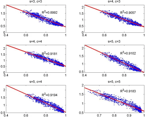
Fig. 5 shows that high STC values are associated with times of high average SST. Looking at the STC versus the standard deviation of the SST values shows a clear contrast-ing relationship: high STC values are associated with a low standard deviation of the SST (Fig. 6). This relationship suggests that the ocean has a high relative degree of spa-tial heterogeneity (STC) during the hot summer months and low spatial heterogeneity (yet high overall (non-spatial) vari-ance) in the cooler months. The high STC during the summer months is due to relatively weaker winds and high precipi-tation, allowing for more localized and heterogeneous SST patterns to dominate (Fig. 2c, d). The high STC of summer months could also be due to the typhoons whose short dura-tions in contrast to the rest of the year do not introduce much variability to the data at this weekly temporal resolution. In contrast, the prevailing weather patterns during the winter months allow for large contiguous patches of cool waters to form due either to atmospheric cooling or to vertical mix-ing through the weak thermocline. The formation of these patches are however highly variable with the strength of the prevailing wind (Fig. 2a, b).
The high (positive) correlation between STC values and the mean of the SST time-slice prompted us to investigate if STC could provide additional insights into the data than those provided by simply plotting the SST mean. Fig. 7 and Supplement Figs. 3 and 4 show that although STC (red lines) and SST (green and blue lines) have the same periodic pat-tern, STC is different from SST during the middle of the year when the STC and SST are high, i.e., during the SW
mon-Fig. 5. Scatter plot of STC (x-axis) vs mean of SST time-slice (y-axis) for each set ofsandcin Fig. 4.
Fig. 6. Scatter plot of STC (x-axis) vs standard deviation of the SST time-slice (y-axis) for each set ofsandcin Fig. 4.
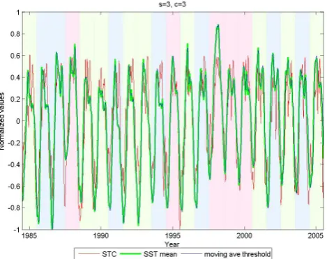
soon and succeeding inter-monsoon. This indicates that dur-ing this period, the spatio-temporal complexity of the SST data is dominated by forces other than the temporal changes in temperature. On the other hand, STC follows SST during the inter-monsoon preceding the SW monsoon.
Fig. 7. The STC plots (red) together with the mean of the slice win-dows used in STC calculations (green) and the thresholds obtained by taking the mean of the 5 weeks centered at the current week be-ing analyzed (blue). Each dataset (STC, SST mean and SST movbe-ing ave threshold) are mean-centered and divided by their maxima. El Ni˜no years are highlighted in blue, La Ni˜na in red and normal years in green.
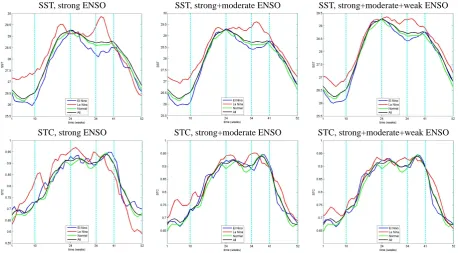
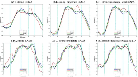
To further analyze in detail how the STC and SST compare during the Philippine seasons, we plotted their average val-ues at each week in Fig. 8. The average of the valval-ues in Fig. 7 corresponds to the right-most column in in Fig. 8, where all strong, moderate and weak ENSO years are used. We also obtained the average of strong ENSO years (left column) and strong plus moderate ENSO years (middle column). A com-parison of the upper and lower panels reveals a contrasting behavior of the STC and SST during the middle of the year. SST is higher during the SW monsoon than during the inter-monsoon following it. On the other hand, STC is higher during the end of the SW monsoon (and at the start of the inter-monsoon), than during the start of the SW monsoon.
Note that in all plots in Fig. 8, La Ni˜na (in red) appears to be distinct from the other years. This could be due to the smaller number of years used in the study. On the left-most column, only one strong La Ni˜na year was used (1988), com-pared to two years (1991 and 1997) for El Ni˜no, while on the middle column, 3 years were used for La Ni˜na compared to 6 years for El Ni˜no years. Although La Ni˜na appears distinct from the other years even when strong, moderate and weak years were used (right-most column), the difference shows in both the SST average (top) and STC average (bottom) and thus this could be attributed to the usual higher temperatures of La Ni˜na years. A study using a longer time-span with more La Ni˜na annotated years is needed to determine if the spatio-temporal complexity of La Ni˜na is indeed different from those of the other years.
To determine if the higher STC values at the end of the SW monsoon in Fig. 8 are due to the STC parameters, we plotted results for different parameters in Supplement Fig. 5, with s=5,c=3,j=2,s=5,c=5,j=2 ands=5,c=5,j=5. A moving average threshold of 11 weeks (j=5) slightly di-minished the higher STC values at the end of the SW mon-soon, but is still present. The 21-year plots of the STC and SST using different STC parameters in Supplement Figs. 3 and 4 also show that the STC values are higher during the latter part of the SW monsoon.
We divided the 52-week period into 5 intervals, chosen by visually inspecting the SST plots in Fig. 8 and manually choosing points where the plot changes direction. The in-tervals we obtained are: weeks 1–10, 11–24, 25–34, 35–41 and 42–52, and are indicated by vertical grid-lines in Fig 8. These intervals roughly coincide with the Philippine seasons (Table 2): weeks 11–24 are in the inter-monsoon from NE to SW, weeks 25–34 are in the SW monsoon, weeks 35–41 are in the inter monsoon from SW to NE, and weeks 42–52 together with weeks 1 to 10 are in the NE monsoon. Not all intervals match the peaks or valleys in the STC plots (lower panels of Fig. 8), indicating that although STC fol-lows the overall pattern of SST, it captures signals other than those from temporal changes of the temperature. To in-vestigate in more detail, we mean-centered and normalized the SST and STC averages (from Fig. 7), and plotted the STC and SST values on the same axis. Fig. 9 and Supple-ment Fig. 6 show that STC and SST are are almost identical during the inter-monsoon which leads to the SW monsoon (weeks 11–24), STC is higher than SST during the inter-monsoon (following the SW inter-monsoon, weeks 35–41), and during the start of the NE monsoon, the STC values drop faster than SST. A one-tailed t-test of the SST values during weeks 11–24 and weeks 25–34 yielded a p-value of 4.8e-2 for El Ni˜no (strong+moderate+weak), 1.9e-4.8e-2 for La Ni˜na (strong+moderate+weak), 2.1e-3 for normal years, and 5.2e-3 for all years. Atα=0.05 significance level, all tests sup-ported our observation that SST is higher during the SW monsoon than during the following inter-monsoon. We next performed a one-tailed t-test of the SST and STC values dur-ing the inter-monsoon (after SW monsoon, weeks 35–41), and obtained the following values: 1.2e-5 for El Ni˜no, p-value=3.0e-1 for La Ni˜na, 2.4e-6 for normal, and 1.9e-6 for all years. At the same significance level, El Ni˜no, normal and all years rejected the null hypothesis, supporting our obser-vation that STC is higher during this period. It can be seen in Fig. 9 and Supplement Fig. 6 that the STC and SST val-ues of La Ni˜na during the SW monsoon and inter-monsoon are not much different. The relationships between SST and STC for each of the intervals are investigated in more detail in Supplement Fig. 7.
Z. T. Botin et al.: Spatio-Temporal Complexity analysis of Philippine SST 941
SST, strong ENSO SST, strong+moderate ENSO SST, strong+moderate+weak ENSO
STC, strong ENSO STC, strong+moderate ENSO STC, strong+moderate+weak ENSO
Fig. 8. Yearly average of the SST (top row) and STC values (bottom row). Strong El Ni˜no and La Ni˜na years (left column), strong + moderate (middle column) and strong + moderate + weak ENSO years are used (Table 1). The 399×365 Philippine region SST values on each week were averaged, then at each week, the values from all the years were averaged. The same was done for the STC values except there was no need to average over a spatial region. In all plots, the normal and all year groups do not vary. STC parameters:s=3,c=3,
j=2, overlapping time-slices.
Fig. 9. The STC and SST yearly average values (as computed in Fig. 8) were mean-centered and divided by the maximum value. For El Ni˜no and La Ni˜na, all strong, moderate and weak years were used.
eigenvectors. Thus, we created a data matrix with 399
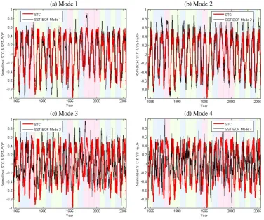
× 365 rows (corresponding to the spatial coordinates of the SST measurements) and 1092 columns (corresponding to the weekly measurements), and computed its SVD de-composition. Rows corresponding to points on land were deleted from the matrix in order to save memory. The time-dependent amplitudes were obtained directly from the decomposition. We then plotted the four most dominant time-dependent amplitudes together with the STC values in Fig. 10. The figure shows that STC has the same periodic pattern as EOF modes 1 and 2 for the SST data. The orthogo-nality of modes 1 and 2 in the figure is not apparent since we mean-centered the time-dependent amplitudes. Differences between the EOF and STC could be seen with modes 3 and 4. Similar to the SST plots, mode 1 of the SST EOF shows a different profile than the STC during the SW monsoon (see also the plots of the STC and SST EOFs in the next section).
3.2 EOF analysis of the Philippine region STC
(a) Mode 1 (b) Mode 2
(c) Mode 3 (d) Mode 4
Fig. 10. The STC over 21 years (s=3,c=3,j=2, overlapping time-slices) together with the time-dependent amplitudes of first four EOF modes (a–d) of the SST. The STC and the time-dependent amplitudes of the SST were mean-centered and divided by their maxima. El Ni˜no years are highlighted in blue, La Ni˜na in red and normal years in green.
groups. This percentage is computed by taking the ratio
PK i=1λi
/PM
i=1λi
, where λi are the eigenvalues from the EOF calculations (arranged in decreasing order).
The time dependent amplitudes (Eq. 4) of the dominant modes are plotted in Fig. 11, while the time dependent am-plitudes of mode 2 are depicted in Fig. 12. We obtained sim-ilar results using different moving window threshold sizes, different time slices,s=3,4,5, and different moving thresh-old averages,j=0,...,3 (Supplement Figs. 8 and 9). Also plotted in Figs. 11 and 12 are the time dependent amplitudes from the EOF analysis of the SST data. The EOF of the SST was computed by obtaining the average SST values of the whole region at each time point, and then performing EOF calculations as in the STC data (which is different from, and not as computationally intensive, as the calculations of the SST EOF in Fig. 10).
Figure 11 reflects the observation from the time-history STC plots that the STC is lowest at the start and at the end of each year, during the NE monsoon (Fig. 8), and is high during the SW monsoon. Also, the SST is higher during the start of the SW monsoon, while the STC is higher during the end of the SW monsoon.
Table 3. The percentage of the variability of the set captured by the first four EOF modes for the Philippine region STC during the El Ni˜no, La Ni˜na and Normal years (top) and for each of the thermal regions (bottom). For El Ni˜no and La Ni˜na, all strong, moderate and weak ENSO years were used. STC parameters: s=3,c=3 and moving average thresholdj=2.
Variability Captured by FirstKModes
K 1 2 3 4
EOF of Philippine Region STC
El Ni˜no 88.7% 93.2% 95.8% 97.3% La Ni˜na 84.8% 92.5% 96.8% 98.6% Normal 89.3% 92.4% 95.3% 97.0% All 86.6% 89.2% 91.5% 93.6%
EOF of Thermal Region STC
Z. T. Botin et al.: Spatio-Temporal Complexity analysis of Philippine SST 943
SST, strong ENSO SST, strong+moderate ENSO SST, strong+moderate+weak ENSO
STC, strong ENSO STC, strong+moderate ENSO STC, strong+moderate+weak ENSO
Fig. 11. Time-dependent amplitudes of the most dominant mode obtained from EOF analysis of SST (top) and STC values (bottom). Strong El Ni˜no and La Ni˜na years (left column), strong + moderate (middle column) and strong + moderate + weak ENSO years are used (Table 1). In all plots, the normal and all year groups do not vary (Table 1). STC parameters:s=3,c=3 and moving average thresholdj=2.
Figure 12 suggests that EOF mode 2 could potentially ferentiate ENSO years since El Ni˜no and La Ni˜na have dif-ferent peaks (see the right-most column of the figure con-taining strong, moderate and weak ENSO years), and that the profiles of the STC and SST differ. An analysis of EOF mode 2 using more years (say 30 years instead of 21 years used in this study) which includes more strong ENSO years could provide further insights in the use of STC in identify-ing ENSO years.
3.3 EOF analysis of the thermal region STCs
We next sought to determine if the STC could detect differ-ences between the spatio-temporal patterns of regions which are affected by different oceanographic conditions. The clus-tering methodology yielded six thermal regions whose loca-tions are indicated in Fig. 2. Thermal region 1 is located north of Luzon, region 2 is located in the northern part of the Philippine Sea, region 3 is located in the southern part of the Philippine Sea, region 4 is in the west of the Philippines facing the South China Sea, region 5 is in the Sulu Sea and region 6 is south of Mindanao facing the Sulawesi/Celebes Sea.
For each thermal region, the plot of the STC and the mean SST of the time-slice, together with the moving average threshold used in converting the SST data to binary, are plot-ted in Fig. 13 (plots using other STC parameters are given
in Supplement Figs. 10, 11, 12). Unlike the analogous fig-ure for the whole Philippine region in Fig. 7, the STC and SST plots of the thermal regions are distinct. However, the 21-year plots could not reveal the differences in the thermal regions. Furthermore, unlike the Philippine region, the lin-ear relationship between the STC value at a certain week and the mean of the time slice used in computing the STC value of that week is not present in the scatter plots of the thermal regions (Supplement Figs. 13 and 14).
We next employed EOF analysis on the STC of each ther-mal region. The time dependent amplitudes (Eq. 4) of the first 4 dominant modes are plotted in Fig. 14 . Results using different time slices (s=3,4,5), moving average threshold j=0,1,2,3 and moving cube size ofc=3 for the first two modes are similar and are presented in Supplement Figs. 15 and 16. The percent of variability captured by the most dom-inant mode of each region is around 20%, which is much lower than the whole country EOF (Table 3).
SST, strong ENSO SST, strong+moderate ENSO SST, strong+moderate+weak ENSO
STC, strong ENSO STC, strong+moderate ENSO STC, strong+moderate+weak ENSO
Fig. 12. Time-dependent amplitudes of the second most dominant mode obtained from EOF analysis of SST (top) and STC values (bottom). Strong El Ni˜no and La Ni˜na years (left column), strong + moderate (middle column) and strong + moderate + weak ENSO years are used (Table 1). In all plots, the normal and all year groups do not vary (Table 1). STC parameters: s=3,c=3 and moving average threshold
j=2. There is only one strong La Ni˜na year hence its EOF does not have mode 2 (left column).
at this time. This causes the different STC pattern from the other thermal regions, but since the signals (with the Ku-rushio intrusion being stronger than the NE monsoon) change with monsoon, then its EOF follows that of the Philippine region EOF (which is monsoon driven). Therefore, even though the EOF of Thermal region 1 follows the Philippine region, the underlying physical events are different. Lastly, we note the very different patterns in the second EOF mode for each of the thermal regions. These differences suggest that it may be possible to differentiate the dynamics of the regions with this mode.
The time-dependent amplitudes of the EOF analysis of the thermal regions grouped according to ENSO years are pre-sented in Supplement Figs. 17 and 18 (using strong and mod-erate ENSO years) and Supplement Figs. 19 and 20 (using strong, moderate and weak ENSO years).
4 Conclusions
We have discussed the prevailing meteorology and oceanog-raphy system of the Philippines as it correlates with observa-tions from the STC signals. STC analysis of the Philippine SST data was able to capture the two monsoonal weather systems experienced by the country every year. In partic-ular: (1) there was a predominant seasonal variation in the
yearly STC plots of the Philippine SST data with STC be-ing relatively lower durbe-ing the start and towards the end of the year, (2) the highest variability of STC values for most regions was found during the inter-monsoon, and (3) the rel-atively weaker SW monsoon during the middle of the year coincides with higher STC values.
The high STC (>0.90) observed in the Philippine region during the middle of each year is indicative of scale-invariant dynamics in the SST at this time. This is perhaps a sign that the system is maintained at the edge of a phase-transition or in a self-organized critical state.
The second most-dominant EOF of the Philippine region STC seems to indicate that this mode could potentially dif-ferentiate ENSO years since the time-dependent amplitudes are clearly different between the EOF of the STC and the EOF of the SST (which is not the case with mode 1), and since the time-dependent amplitudes of the the second most dominant mode of the EOF-STC of each ENSO group are distinguishable. This could be investigated by including a longer number of years in the study.
Z. T. Botin et al.: Spatio-Temporal Complexity analysis of Philippine SST 945
Fig. 13. The STC of each thermal region, plotted with the mean of the time slice used in computing the STC, and with the moving average threshold. The STC, slice window mean and the moving average threshold are fist mean-centered and then divided by their maximum to normalize the values. Overlapping time slices,s=3,j=2,c=3. El Ni˜no years are highlighted in blue, La Ni˜na in red, and normal years in green.
that could be used for studying the STC values. Therefore, thermal region analysis suggests that if ever STC is not able to determine temporal differences from a given data set, one can zoom in on specific areas and explore if STC will be able to present temporal variations at a finer scale.
Although STC was applied only to binary data in this pa-per, the formula for STC can be modified to be able to in-clude application to multi-valued matrices. To do this, one can consider a matrix ofn values where each matrix entry depends on the satisfaction of one ofnconditions. In addi-tion, we also showed that despite this binary limitaaddi-tion, STC for the Philippine wide SSTs was still able to differentiate El Ni˜no from La Ni˜na and normal years. We conclude that the STC measure is thus potentially useful for the analysis of
many different types of remotely sensed data in which the ob-jective is to detect and characterize areas of spatio-temporal variability in the environment.
Supplementary material related to this article is available online at:
(a) Mode 1 (b) Mode 2
(c) Mode 3 (d) Mode 4
Fig. 14. The first four EOF modes of the thermal regions usings=3,c=3 and a moving window average threshold of 5 weeks.
Acknowledgements. The authors would like to thank
William Skirving of NOAA-CRW and WB/GEF-RSWG for providing us with the 4 km dataset. We would also like to acknowledge the invaluable assistance of Eileen Penaflor for the pre-processing of the data. Finally, we express gratitude to Ed-uardo Mendoza of the University of Munich, Physics Department and Center for Nano-Science for inspiring this inter-disciplinary collaboration.
Edited by: J. M. Huthnance
References
Andrienko, Y. A., Brillantov, N. V., and Kurths, J.: Complexity of two-dimensional patterns, Eur. Phys. J., 15, 539–546, 2000. Atmanspacher, H.: A Semiotic Approach to Complex Systems, in:
Aspects of Automatic Text Analysis, edited by: Mehler, A. and K¨ohler, R., 79–91, Springer, Berlin, 2007.
Bak, P. and Chen, K.: Self-organized criticality, Scientific Ameri-can, 264, 46–53, 1991.
Banks, H., del Rosario, R., and Tran, H.: Experimental Implemen-tation of POD Based Reduced Order Controllers on Cantilever Beam Vibrations, IEEE Transactions on Control Systems Tech., 10, 717–726, 2002.
Botin, Z. T.: Spatio-Temporal Complexity of the Sea Surface Tem-peratures of the Philippines, MS Thesis, College of Science, Uni-versity of the Philippines Diliman, 2009.
Bruno, J. F., Selig, E. R., Casey, K. S., Page, C. A., Willis, B. L., Harvell, C. D., Sweatman, H., and Melendy, A. M.: Thermal Stress and Coral Cover as Drivers of Coral Disease Outbreaks, PloS Biol, 5, e124, 2007.
Buddemeier, R. W., Smith, S. V., Swaney, D. P., Crossland, C. J., and Maxwell, B. A.: Coastal typology: An integrative “neutral” technique for coastal zone characterization and analysis, Estuar. Coast. Shelf S., 77, 197–205, 2008.
Centurioni, L. C., Niler, P. P., and Lee, D. K.: Observations for inflow of Philippine sea surface water into the South China Sea through the Luzon Strait, J. Phys. Oceanogr., 34, 113–121, 2004. Emery, W. J. and Thomson, R. E.: Data Analysis Methods in Phys-ical Oceanography: Second and Revised Edition, Elsevier, 2001. Glynn, P. W. and D’Croz, L. D.: Experimental Evidence for High Temperature Stress as the Cause of El Ni˜no-Coincident Coral Mortality, Coral Reefs, 8, 181–191, 1990.
Golden Gate Weather Services: http://ggweather.com/enso/oni.htm, last access: March 2010, 2010.
Goldenfeld, N.: Lectures on Phase Transitions and the Renormal-ization Group, Addison-Wesley, Boston, 1992.
Z. T. Botin et al.: Spatio-Temporal Complexity analysis of Philippine SST 947
Lesser, M. P., Stochaj, W. R., Tapley, D. W., and Shiek, J. M.: Bleaching in Coral Reef Anthozoans: Effects of Irradiance, Ul-traviolet Radiation, and Temperature on the Activities of Protec-tive Enzymes against AcProtec-tive Oxygen, Coral Reefs, 8, 225–232, 1990.
MacArthur, R. H.: Fluctuation of Animal Populations and a Mea-sure of Community Stability, Ecology, 36, 533–536, 1955. National Oceanographic Data Center: 4 km Pathfinder Version
5.0 User Guide, http://www.nodc.noaa.gov/sog/pathfinder4km/ userguide.html, 2008.
Nsakanda, A. L., Price, W. L., Diaby, M., and Gravel, M.: Ensuring Population Diversity in Genetic Algorithm: A Technical Note with Application to the Cell Formation Problem, Eur. J. Oper. Res., 178, 634–638, 2007.
Parrott, L.: Quantifying the Complexity of Simulated Spatiotempo-ral Population Dynamics, Ecol. Complex., 2, 175–184, 2005. Parrott, L., Proulx, R., and Thibert-Plante, X.: Three dimensional
metrics for the analysis of ecological data, Ecol. Inform., 3, 343– 353, 2008.
Pe˜naflor, E. L., Skirving, W. J., Strong, A. E., Heron, S. F., and David, L. T.: Sea-surface temperature and thermal stress in the Coral Triangle over the past two decades, Coral Reefs, doi:10.1007/s00338-009-0522-8, 2009.
Pratchett, M. S., Wilson, S. K., and Baird, A. H.: Declines in the Abundance of Chaetodon Butterflyfishes Following Exten-sive Coral Depletion, J. Fish Biol., 69, 1269–1280, 2006.
Reichl, L. E.: A Modern Course in Statistical Physics, 2nd ed., Wi-ley & Sons, NewYork, 1998.
Shalizi, C. R. and Shalizi, K. L.: Quantifying Self-Organization in Cyclic Cellular Automata, in: Noise in Complex Systems and Stochastic Dynamics, Proceedings of SPIE, vol. 5114, edited by: Shcimansky-Geier, L., Abbott, D., Neiman, A., and den Broeck, C. V., Bellingham, Washington, 2003.
Shaw, P. and Chao, S.: Surface circulation in the South China Sea, Deep-Sea Res. Pt. I, 41, 1663–1683, 1994.
Strong, A. E., Barrientos, C., Duda, C., and Sapper, J.: Improved Sattelite Techniques for Monitoring Coral Reef Bleaching, Proc 8th International Coral Reef Symposium, Panama City, Panama, 1495–1498, 1996.
Turcotte, D. L.: Fractals and chaos in geology and geophysics, Cambridge University Press, Cambridge, 1997.
Wackerbauer, R., Witt, A., Atmanspacher, H., , Kurths, J., and Scheingraber, H.: A comparative classification of complexity measures, Chaos, Solitons and Fractals, 4, 133–173, 1994. Williams, F. R., Jung, G. H., and Englebreston, R. E.: Forecasters