www.atmos-meas-tech.net/8/2473/2015/ doi:10.5194/amt-8-2473-2015
© Author(s) 2015. CC Attribution 3.0 License.
Level 2 processing for the imaging Fourier transform spectrometer
GLORIA: derivation and validation of temperature and trace gas
volume mixing ratios from calibrated dynamics mode spectra
J. Ungermann1, J. Blank1, M. Dick1, A. Ebersoldt2, F. Friedl-Vallon3, A. Giez4, T. Guggenmoser1,*, M. Höpfner3, T. Jurkat5, M. Kaufmann1, S. Kaufmann5, A. Kleinert3, M. Krämer1, T. Latzko3, H. Oelhaf3, F. Olchewski6, P. Preusse1, C. Rolf1, J. Schillings1, O. Suminska-Ebersoldt3, V. Tan1, N. Thomas1, C. Voigt5, A. Zahn3, M. Zöger4, and M. Riese1
1Institut für Energie- und Klimaforschung – Stratosphäre (IEK-7), Forschungszentrum Jülich GmbH, Jülich, Germany 2Institut für Prozessdatenverarbeitung und Elektronik, Karlsruher Institut für Technologie, Karlsruhe, Germany 3Institut für Meteorologie und Klimaforschung, Karlsruher Institut für Technologie, Karlsruhe, Germany 4Flugexperimente, Deutsches Zentrum für Luft- und Raumfahrt, Oberpfaffenhofen, Germany
5Institut für Physik der Atmosphäre, Deutsches Zentrum für Luft- und Raumfahrt, Oberpfaffenhofen, Germany 6Institute for Atmospheric and Environmental Research, University of Wuppertal, Wuppertal, Germany *now at: European Space Agency, Noordwijk, the Netherlands
Correspondence to: J. Ungermann ([email protected])
Received: 19 September 2014 – Published in Atmos. Meas. Tech. Discuss.: 2 December 2014 Revised: 29 March 2015 – Accepted: 24 May 2015 – Published: 17 June 2015
Abstract. The Gimballed Limb Observer for Radiance Imag-ing of the Atmosphere (GLORIA) is an airborne infrared limb imager combining a two-dimensional infrared detec-tor with a Fourier transform spectrometer. It was operated aboard the new German Gulfstream G550 High Altitude LOng Range (HALO) research aircraft during the Trans-port And Composition in the upper Troposphere/lowermost Stratosphere (TACTS) and Earth System Model Validation (ESMVAL) campaigns in summer 2012.
This paper describes the retrieval of temperature and trace gas (H2O, O3, HNO3) volume mixing ratios from GLORIA dynamics mode spectra that are spectrally sampled every 0.625 cm−1. A total of 26 integrated spectral windows are employed in a joint fit to retrieve seven targets using con-secutively a fast and an accurate tabulated radiative trans-fer model. Typical diagnostic quantities are provided includ-ing effects of uncertainties in the calibration and horizontal resolution along the line of sight. Simultaneous in situ ob-servations by the Basic Halo Measurement and Sensor Sys-tem (BAHAMAS), the Fast In-situ Stratospheric Hygrometer (FISH), an ozone detector named Fairo, and the Atmospheric chemical Ionization Mass Spectrometer (AIMS) allow a
val-idation of retrieved values for three flights in the upper tro-posphere/lowermost stratosphere region spanning polar and sub-tropical latitudes. A high correlation is achieved between the remote sensing and the in situ trace gas data, and discrep-ancies can to a large extent be attributed to differences in the probed air masses caused by different sampling characteris-tics of the instruments.
This 1-D processing of GLORIA dynamics mode spectra provides the basis for future tomographic inversions from cir-cular and linear flight paths to better understand selected dy-namical processes of the upper troposphere and lowermost stratosphere.
1 Introduction
2474 J. Ungermann et al.: Level 2 processing for GLORIA dynamics mode
the subtropical jet forms typically a barrier for troposphere-stratosphere exchange, which can weaken in the presence of breaking Rossby waves and thus allow for isentropic trans-port (e.g. Chen, 1995; Berthet et al., 2007). Especially during summer, when the jet is weak, the UTLS over Europe con-sists of a cascade of small filaments (Postel and Hitchman, 1999; Ungermann et al., 2013; Gille et al., 2014).
Examining this region with airborne in situ instruments gives precise and accurate information on the trace gas dis-tribution confined to the flight path but allows thus only for sketchy coverage. Using remote sensing instruments with a high vertical resolution such as limb sounders offers a much more complete spatial picture. Observing the atmosphere with limb sounders from space (e.g. Offermann et al., 1999; Hegglin et al., 2009; Gille et al., 2008; Fischer et al., 2008; Peevey et al., 2014) has greatly increased our knowledge of the dynamical and chemical structure of the atmosphere, but satellite-born instruments lack the vertical resolution to observe the strong vertical gradients occurring around the tropopause. Airborne limb sounders close the gap between in situ and space instruments and thus allow for the obser-vation of small-scale structures such as the tropopause inver-sion layer (Birner, 2006; Riese et al., 2014).
The Gimballed Limb Observer for Radiance Imaging of the Atmosphere (GLORIA) is the first realisation of the limb-imagining technique originally proposed for satellite applica-tions (Riese et al., 2005; Friedl-Vallon et al., 2006). The in-strument combines an imaging detector with a Fourier trans-form spectrometer. To operate on an aircraft, it is placed in a gimbal (a cardanic frame), which is used to stabilise the pointing against movements of the carrier and to ad-just the viewing direction. It offers a high vertical resolu-tion of down to 250 m and, in combinaresolu-tion with tomographic measurement patterns, even the 3-D reconstruction of at-mospheric structures is feasible (Kaufmann et al., 2015). GLORIA can be tuned between the highly spatial “dynam-ics mode” and the highly spectral “chemistry mode” res-olution (see Sect. 2). GLORIA was first operated on the Geophysica research aircraft during the Esa Sounder Cam-paign (EsSenCe; Kaufmann et al., 2013) based in Kiruna, Sweden, in 2011 with a limited number of measured profiles. The first deployment with extended data coverage took place during the TACTS (Transport And Composition in the upper Troposphere/lower most Stratosphere) and ESMVal (Earth System Model Validation) campaigns in the High Altitude LOng Range (HALO) aircraft (a Gulfstream G550) in sum-mer 2012.
This paper provides a complete picture of the 1-D level 2 processing of GLORIA “dynamics mode” data. It continues the work presented by Kaufmann et al. (2015) by also pro-viding the important tropospheric tracer H2O with high sen-sitivity in the lower stratosphere. The selection of spectral re-gions has been greatly improved upon by incorporating new insights into instrument behaviour. Further, the accuracy of the retrievals has been improved by employing a more
ac-curate radiative transfer model. Lastly, a detailed validation is presented that exploits the available in situ instrumentation aboard HALO. While the described 1-D retrievals are inaccu-rate in the presence of horizontal gradients (in contrast to the 3-D tomography of Kaufmann et al., 2015), they do not re-quire dedicated flight patterns as tomography and can quickly provide an overview picture of the dynamic situation.
First, the instrument will be described followed by a de-scription of the “dynamics mode” level 2 processor and the used configuration designated V1.00 for the GLORIA data processing. The paper proceeds by presenting the derived distributions of temperature and trace gas mixing ratios of H2O, O3, and HNO3from 7 to 15 km altitudes above north-ern Europe on 26 September 2012. After the discussion of systematic errors, the retrieved trace gas distributions are val-idated against simultaneous in situ observations on HALO during three flights in September 2012 covering polar, mid-latitude, and subtropical regions.
2 GLORIA instrument
The GLORIA instrument is a Fourier transform spectrometer (FTS) with a HgCdTe infrared image detector array (cooled to an operating temperature of 50 K) allowing to take up to 16 384 spectra simultaneously. To reduce the read out time, only 6144 of these are currently used. The usable spectral coverage ranges from approximately 780 to 1400 cm−1while the spectral sampling can be adjusted quite freely (see Ta-ble 1). During the TACTS and ESMVAL campaigns, two spectral sampling configurations were used: 0.625 cm−1 (dy-namics mode) and 0.0625 cm−1(chemistry mode). The de-tector has a fixed pixel pitch of≈1.9 arcmin (0.032◦), which
corresponds to a vertical sampling of≈140 m at a tangent point 5 km below flight altitude. GLORIA is mounted in a gimbal that, on the one hand, allows to counterpoise move-ments of the aircraft during the image acquisition and, on the other hand, to point the instrument at different azimuth an-gles covering slightly less than 90◦. The latter enables 3-D tomographic retrievals where the same air mass is measured from multiple viewing angles (Ungermann et al., 2011; Kauf-mann et al., 2015).
3 Level 2 processing
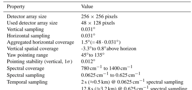
el-Table 1. Key instrument characteristics and properties (Friedl-Vallon et al., 2014).
Property Value
Detector array size 256×256 pixels Used detector array size 48×128 pixels
Vertical sampling 0.031◦
Horizontal sampling 0.031◦
Aggregated horizontal coverage 1.5◦(= 48·0.031◦) Vertical spatial coverage -3.3◦to 0.8◦above horizon Yaw pointing range 45◦to 135◦
Pointing stability (vertical, 1σ) 0.012◦
Spectral coverage 780 cm−1to 1400 cm−1 Spectral sampling 0.0625 cm−1to 0.625 cm−1
Temporal sampling 2 s (≈0.5 km) @ 0.0625 cm−1spectral sampling 12.8 s (≈3.2 km) @ 0.625 cm−1spectral sampling
evation angles (that is tangent altitudes) to the geophysical quantities of temperature, trace gas volume mixing ratios, and extinction values. This forms an ill-posed problem that is approximated by a well posed one by means of a Tikhonov-type regularisation (Tikhonov and Arsenin, 1977).
Let F:Rn7−→Rm, n, m∈N, be a (forward) model that maps a discrete representation of the atmospheric statex∈
Rn onto a set of radiances. The set of (imperfect)
measure-ments is represented by a vector y∈Rm, and the assumed (prior) state of the atmosphere is given asxa∈Rn.
Approx-imating the behaviour of the instrument noise by a Gaussian error covariance matrix S∈Rm×mand the vertical correla-tion of atmospheric state variables by a Gaussian covariance matrix Sa∈Rn×n, the original problem is approximated by
a minimisation problem:
J (x)=(F(x)−y)TS−1(F(x)−y)
+(x−xa)TSa−1(x−xa)−→min. (1) This problem can be efficiently solved by quasi Newton-type methods, in our case a truncated conjugate gradient-based trust–region scheme (Ungermann, 2013).
3.1 Retrieval targets
The aim of the inversion is here to retrieve the primary tar-gets of temperature, water vapour (H2O), ozone (O3), and nitric acid (HNO3). The secondary targets of carbon tetra-chloride (CCl4), CFC-11, and CFC-12 are retrieved to reduce systematic errors due to these background gases. The Antarc-tic flight requires additionally the derivation of chlorine ni-trate (ClONO2) due to the large encountered volume mixing ratios (VMRs). In addition, five different aerosol extinction profiles are retrieved, whereby each aerosol is applied only to a non-overlapping spectral region, and it is assumed that the optical characteristics of an aerosol remains approximately constant over its applicable wavenumber range (see Table 2). The listed integrated spectral windows (ISWs) used for the
retrievals were selected by a genetic algorithm, which iden-tifies the location and width of ISWs that maximises the in-formation gain. The algorithm recombines initially randomly selected sets of ISWs preferring ”good” sets and thus iden-tifies a (nearly) optimal set much faster than a simple brute force search. Details are given by Blank (2013). The resulting windows were then modified to mitigate discovered instru-ment artefacts such as imperfectly compensated emissions of the outer window due to fast temperature changes. Gener-ally, the volume mixing ratio of trace gases is retrieved. But for H2O, the logarithm of the VMR is retrieved instead of the unmodified VMR. From a statistical point of view, this assumes that H2O VMRs follow a log-normal distribution, which can be justified in the target altitude range from ra-diosonde measurements (e.g. Schneider et al., 2006). A full list of atmospheric quantities taken into account in the re-trieval is given in Table 4.
The retrieval grid has a sampling distance of 125 m be-tween the surface and 18 km altitude, from where on the sam-pling becomes increasingly sparse: 1 above 18 km, 2 above 24 km, and 4 above 30 km, with 60 km being the highest alti-tude. All targets are retrieved up to 20 km altitude except for O3and HNO3, which are retrieved up to 60 km.
3.2 Regularisation and model a priori data
2476 J. Ungermann et al.: Level 2 processing for GLORIA dynamics mode
Table 2. A list of integrated spectral windows (ISW) employed and their spectral range. The last four columns shown the bias and SD of the band and monochromatic model compared to RFM.
aerosol band monochromatic
ISW index range (cm−1) bias (‰) stddev (‰) bias (‰) stddev (‰)
0 0 790.625–791.250 2.851 0.762 0.074 0.011
1 0 791.875–792.500 −1.431 0.282 0.073 0.012
2 0 793.125–793.750 −2.075 0.531 0.160 0.019
3 0 794.375–795.000 1.634 0.490 0.124 0.019
4 0 795.625–796.250 −0.380 1.526 0.045 0.010
5 0 796.875–797.500 −0.028 0.740 −0.017 0.010
6 0 798.125–798.750 6.513 5.082 −0.108 0.030
7 0 799.375–799.375 1.168 2.487 −0.089 0.026
8 1 845.000–849.375 −0.016 0.251 0.047 0.008
9 1 850.000–854.375 −0.924 0.229 −0.238 0.023
10 1 855.000–859.375 −0.739 0.231 −0.177 0.027
11 2 883.750–888.125 −1.683 0.134 0.012 0.003
12 2 892.500–896.250 −0.998 0.099 −0.017 0.004
13 2 900.000–903.125 −0.889 0.144 0.119 0.026
14 2 918.750–923.125 0.233 0.236 0.048 0.017
15 3 956.875–962.500 −2.518 0.861 0.066 0.009
16 3 980.000–984.375 −5.826 0.696 0.076 0.005
17 3 992.500–997.500 −2.909 0.406 0.055 0.004
18 3 1000.625–1006.250 −0.696 0.337 0.023 0.004
19 3 1010.000–1014.375 −0.243 0.179 0.003 0.002
20 4 1388.125–1389.375 3.001 1.910 −0.001 0.013
21 4 1390.000–1391.250 1.102 0.812 0.012 0.024
22 4 1391.875–1393.125 −0.264 0.545 −0.002 0.036
23 4 1393.750–1395.000 0.391 0.476 0.001 0.004
24 4 1395.625–1396.875 0.973 1.418 0.016 0.019
25 4 1397.500–1398.750 −0.932 0.401 0.005 0.022
The precision matrix S−a1is defined as
S−a1=(α0)2LT0L0+(α1)2LT1L1+(α2)2LT2L2, (2) with α0, α1, α2∈R and L0,L1,L2∈Rn×n. The constraint
can be separated into one constraint on the absolute value of retrieved target compared to a (climatological) mean weighted with its standard deviation (SD) and two smooth-ness criteria. The matrix L0thus consists of a diagonal con-taining the reciprocal values of the SDs of the retrieved enti-ties. The matrix L1is a matrix to compute the first derivative of the vectorxiby finite differences (it has -1 is on the main diagonal and 1 is on the first upper side diagonal, except for some rows that would take the difference of different quan-tities or non-neighbouring values). In addition each row of L1 is scaled with the reciprocal of the SD and pcq/(2hi), withcqbeing a quantity q specific correlation length andhi being the vertical distance between the elements of the vec-tor that are being subtracted from each other (Steck and von Clarmann, 2001). Table 3 lists the empirically derived cor-relations lengths. L2is set up similarly to L1but with finite differences approximating the second derivative instead of the first. The sources for a priori values, background values, and SDs are listed in Table 4.
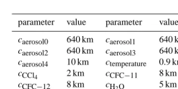
Table 3. Vertical correlation lengths employed for the regularisa-tion.
parameter value parameter value
caerosol0 640 km caerosol1 640 km
caerosol2 640 km caerosol3 640 km
caerosol4 10 km ctemperature 0.9 km
cCCl4 2 km cCFC−11 8 km
cCFC−12 8 km cH2O 5 km
cHNO3 4 km cO3 40 km
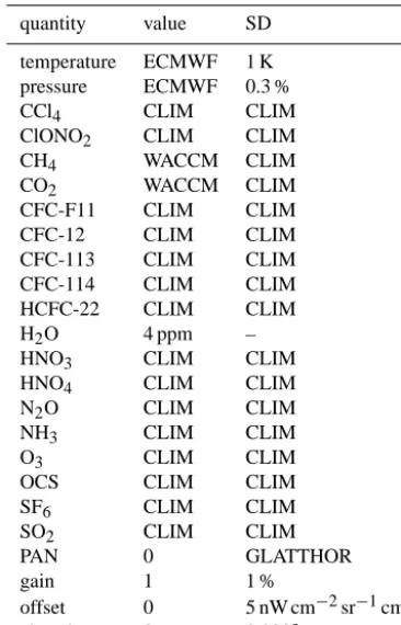
Table 4. Sources for a priori or background values and associated SDs for atmospheric quantities. CLIM refers to the climatology by Remedios et al. (2007), ECMWF and WACCM to the respective models, and GLATTHOR refers to the profile derived by Glatthor et al. (2007), where the derived values are taken as 1-sigma uncer-tainty.
quantity value SD
temperature ECMWF 1 K
pressure ECMWF 0.3 %
CCl4 CLIM CLIM
ClONO2 CLIM CLIM
CH4 WACCM CLIM
CO2 WACCM CLIM
CFC-F11 CLIM CLIM
CFC-12 CLIM CLIM
CFC-113 CLIM CLIM
CFC-114 CLIM CLIM
HCFC-22 CLIM CLIM
H2O 4 ppm –
HNO3 CLIM CLIM
HNO4 CLIM CLIM
N2O CLIM CLIM
NH3 CLIM CLIM
O3 CLIM CLIM
OCS CLIM CLIM
SF6 CLIM CLIM
SO2 CLIM CLIM
PAN 0 GLATTHOR
gain 1 1 %
offset 0 5 nW cm−2sr−1cm
elevation 0 0.023◦
Lastly, the second vertical derivative of the temperature pro-file is constrained by the L2matrix to produce temperature profiles with a smoother lapse rate.
As input to the retrieval, analysis data supplied by the European Centre for Medium-range Weather Forecasts (ECMWF) were used. The ECMWF data is available in six hour time steps with T799/L91 resolution, which cor-responds to a horizontal resolution of ≈0.2◦×0.2◦ and 91 levels in the vertical between the surface and 80 km. For the well-mixed trace gases CO2 and CH4, data from the Whole Atmosphere Community Climate Model, version 4 (WACCM4; Garcia et al., 2007) were employed, mostly to capture the steady increase of CO2 in time that influences retrieved temperatures. The specific parametrisation used for the WACCM4 model run can be found in the publications of Lamarque et al. (2012) and Kunz et al. (2011).
3.3 JURASSIC2 band radiative transfer model
The JURASSIC2 band model is optimised for the fast simu-lation of measurements of coarse or moderate spectral reso-lution. It is thus suitable for the retrieval of large amounts of satellite data (e.g. Hoffmann and Alexander, 2009), but also
for large-scale retrievals as posed by cross-section or tomo-graphic retrievals (Ungermann et al., 2012; Kaufmann et al., 2015).
In a first step, the line-of-sight of a measurement is ray-traced through the 1-D representation of the atmosphere (Hase and Höpfner, 1999). Here, also temperature gradi-ents along the line-of-sight are taken into account. The hori-zontal temperature structure along the line-of-sight found in ECMWF model data is expressed for each altitude layer as difference to the temperature found horizontally at the closest tangent point location. This structure is then used to derive the actual temperature at a given position within an altitude layer in relation to the assumed or derived temperature at the tangent point location. The atmosphere is sampled along the line-of-sight in 5 km steps taking into account atmospheric refraction (Hase and Höpfner, 1999), forming a series of gas cells that are assumed to be homogeneous for simulation pur-poses.
In a second step, the emissivity and source function are computed for each gas cell and used to simulate the mea-sured radiance. The band model uses tabulated optical path values for the typical ranges of atmospheric pressure, tem-perature, and number density values for the employed ISWs (which may be as small as a single spectral sample of GLO-RIA, but usually consist of the arithmetic mean of several neighbouring samples). The tables are generated by the ref-erence forward model (RFM v4.3; Dudhia et al., 2002) us-ing the current HITRAN2012 (Rothman et al., 2013) spectral database including all updates up to June 2014; the accuracy of the JURASSIC2 model is here always taken in reference to the RFM. The tabulated optical path values are generated by convolving monochromatic emissivities with the instru-ment line shape (ILS) and conversion to optical path as a last step. This reversal of integration order makes this less exact, but several orders of magnitude faster than typical line-by-line calculations. For fast radiative transfer calculations, the Curtis–Godson approximation (CGA; Curtis, 1952; Godson, 1953) and the emissivity growth approximation (EGA; Wein-reb and Neuendorffer, 1973; Gordley and Russell, 1981) are employed. For both the CGA and EGA scheme, the optical path of the total column between the instrument up to and including the current homogeneous gas cell is computed to derive the local optical path only by forming the difference to the total optical path up to and including the previous ho-mogeneous gas cell (which was determined in the previous step). A regression-based scheme may also be used to mit-igate any bias introduced by the approximation, but is not needed for the retrieval presented in this paper. Here, simply the arithmetic mean of the values computed by the CGA and EGA methods is used (e.g. Marshall et al., 1994), as a later processing step corrects for any approximation errors intro-duced.
num-2478 J. Ungermann et al.: Level 2 processing for GLORIA dynamics mode
ber density than the transmissivity (due to the highly non-linear exponential function) this reduces the table size signif-icantly for the same accuracy, and thereby reduces memory consumption and increases processing speed.
One ray is computed for each row of the detector. In a sec-ond step, the computed radiances are convolved with a field-of-view function of the instrument determined from labora-tory measurements compensating for optical and electronic effects. Using additional intermediate rays did not change the retrieval results or diagnostics significantly.
The model code uses a tool based on C++ operator over-loading to provide analytically correct derivatives with re-spect to all input parameters with minimal computational overhead (Lotz et al., 2012).
3.4 JURASSIC2 monochromatic radiative transfer model
A new addition to JURASSIC2 is a monochromatic model that serves as a fast reference model. To be rather fast and accurate without becoming too complicated, it uses tabulated extinction cross-sections values on a fine spectral grid. This is considerably faster than actual line-by-line calculations for the spectral regions and emitters used in our retrievals. It is similar in purpose and design to the HIRDLS intermediate reference model (Francis et al., 2006). The spectral grid is configurable but currently uses a sampling of 0.002 cm−1, which is sufficient to resolve individual lines.
The ray tracing and field of view are computed in the same way as for the band model so that the same homogeneous gas cells are used in the computation. However, it is feasible to sample the atmosphere on different grids or use Curtis– Godson means to combine neighbouring samples to larger cells in order to reduce simulation time. In contrast to the band model, the monochromatic model directly computes the emissivity for the local homogeneous gas cells and does not rely on an emissivity growth approximation.
To retain a high accuracy, the extinction cross-sections are not simply linearly interpolated as in the band model, but cubic splines are used. The spline coefficients are not pre-computed, but generated on the fly using local information only to reduce memory consumption and bandwidth. That means that in a first step for each of the four pressure val-ues surrounding the target pressure, a six point cubic spline interpolation in temperature is performed. Afterwards, the fi-nal value is derived from the previously computed four ex-tinction values by means of a four point cubic spline inter-polation in pressure. The boundary condition for each cu-bic spline is that the second derivative should be zero. The pressure log-linear grid uses 42 points between 1017 and 0.0103181 hPa, while temperature is regularly sampled in 5 K steps between 100 and 400 K. It thus uses the same pres-sure and temperature grid as the band model. To reduce mem-ory consumption, only extinction cross-sections for required
temperature and pressure values are read into memory on-demand.
Continua and other smooth functions like the Planck function required in further computations are sampled on a 0.256 cm−1wavenumber grid and are linearly interpolated in between. This greatly increases computation speed with no noticeable degradation of accuracy, especially with respect to the water vapour continua (MT_CKD version 2.5.2; Mlawer et al., 2012). By computing simulated radiances for the re-trieved atmospheres of one flight with both JURASSIC2 models and RFM, the error of the band and the monochro-matic model can be estimated (see Table 2). To provide only a comparison of the radiative transport and not the ray tracing, RFM was only used to compute the spectrally re-solved emissivities of all homogeneous gas cells involved. Larger differences found in previous comparisons (Unger-mann et al., 2012; Griessbach et al., 2013) are largely at-tributable to the different ray tracing schemes and differences in the interpolation of aerosol/extinction (linear compared to log-linear). Typically, the error of the band model increases with decreasing tangent point altitude.
The monochromatic model code was also designed to pro-vide analytically correct derivatives by means of algorithmic differentiation. This allows the model to be used for valida-tion of Jacobian matrices and retrievals. While it could be tuned to be much faster (coarser tables, less accurate interpo-lation, etc.), its primary purpose is to be highly accurate with respect to the (even slower) RFM used for table computa-tion. However, as the campaign data set comprised of 62 960 measured profiles is comparatively small (at least compared to typical satellite experiments), it is feasible to process it in 1-D using the monochromatic model. The retrieval result derived from the band model is used as initial guess for the monochromatic model, thereby reducing the number of re-quired iterations to≈3 down from≈10 on average, whereby only the first iteration changes the result significantly. Using the more accurate model removes a bias in retrieved trace gases, which is most notable for H2O (≈ −6 %) and HNO3 (≈2 %).
3.5 Error analysis
The errors of the retrieved quantities are analysed using a lin-ear approximation (Rodgers, 2000), which can be expressed in the same notation introduced in the beginning of Sect. 3:
xf=Axt+(I−A)xa+G. (3)
The retrieval resultxf∈Rnis the sum of the true atmospheric
statext∈Rnsmoothed by the averaging kernel matrix A∈ Rn×n, the a priori influence, and measurement errors∈Rm.
Whereby
G=S−a1+F0(xf)TS−1F
0 (xf)
−1
and
A=GF0(xf)T, (5)
where F0(xf)is the first derivative (Jacobian matrix) of the forward model F evaluated at the retrieval resultxf.
Given a covariance matrix S∈Rm×m describing the ef-fect of an arbitrary error source on the measurements, the gain matrix G can be used to linearly estimate a covariance matrix describing the effect of this error source on the re-trieval result as GTSG. Such a covariance matrix can be read-ily assembled at least approximately for many systematic er-ror sources using SDs and a reasonable vertical correlation length using an auto-regressive approach (Rodgers, 2000). We distinguish between random errors stemming from mea-surement noise and other, usually systematic, error sources. The measurement noise is taken from theoretical estimates given by Friedl-Vallon et al. (2014). The characterisation of actual noise figures is still in progress; however, initial results indicate that the theoretically predicted values are sufficiently accurate for an error estimation. For ISWs covering several samples, the assumed noise is divided by the square root of the number of spectral samples. In addition, a fixed relative noise component of 0.1 % is assumed for all ISWs.
The error estimate stemming from the noise error source is given as precision value. The errors stemming from mis-represented background gases, uncertainties in spectral line characterisation (taken to be 5 % under the assumption that, statistically, some errors in individual line parameters cancel each other out), uncertainties in instrument attitude, and cal-ibration errors are summed up under the label accuracy. It is assumed that gain and offset errors are spatially uncorre-lated, but spectrally fully correlated (in the absence of a bet-ter characbet-terisation, this provides a worse error estimate than assuming no spectral correlation).
The sum over each row of the averaging kernel matrix A is supplied as measurement contribution. The full width at half max of each row is also computed using linear interpo-lation to provide a measure of the vertical resolution. The smoothing error is not given, as the underlying covariance matrix Sadescribing the prior atmospheric state is far from being accurate in an optimal estimation sense. Still, the ver-tical resolution and measurement contribution can be used to gain insight into the quality of the data. Additionally, the hor-izontal resolution along the line-of-sight is supplied, which can be derived by generating a special averaging kernel ma-trix mapping a 2-D state of the atmosphere along the line-of-sight onto the 1-D retrieval result by multiplying the gain matrix G with a 2-D Jacobian matrix of the forward model with respect to a 2-D representation of the retrieved volume (e.g. von Clarmann et al., 2009; Ungermann et al., 2011).
As the logarithm of H2O VMRs is retrieved, the error anal-ysis also supplies variances with respect to the logarithm. This is somewhat problematic, as the log-normal distribution in VMR space is biased, so that the mean value depends on the assumed SD. To remove this dependency, the median in
VMR space is given instead of the mean; using qlogas the retrieved logarithmic VMR andslogas an associated SD, the conversion from log- to VMR-space is performed with these formulae:
qVMR=exp(qlog) sVMR=exp(qlog) q
exp(slog2 )−1.
4 The TACTS and ESMVal campaigns
The TACTS and ESMVal campaigns using the new German HALO aircraft took place in August and September 2012. GLORIA was deployed during all scientific flights, and it was operational during all but one short flight. The TACTS campaign focused on the UTLS of the extratropics and the transition to the tropics, with the main scientific objective to quantify the change of composition of the UTLS be-tween summer and autumn. Most flights took place over Eu-rope with several additional flights to Cape Verde including stops on the island. ESMVal focused on delivering merid-ional transects covering as many latitudes as possible to gen-erate a comprehensive data set with the purpose of validation and enhancement of chemistry–climate models.
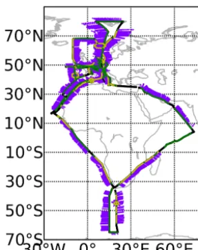
HALO flight paths of all campaign flights are shown in Fig. 1. Combining both campaigns, a broad geographic re-gion was covered: from the Spitsbergen islands at 80◦N
down to close to Antarctica at 65◦S, and from Cape Verde
at 23.6◦W to the Maldives at 73.5◦E. GLORIA took 62 960
spectrally resolved images during the campaigns, consist-ing of 386.8 million spectra coverconsist-ing a horizontal path of≈ 66 000 km. Of these, only a small subset of several thousand profiles has currently been processed. The tangent points of profiles preliminary retrieved using the dynamics mode pro-cessor are shown in Fig. 1. In addition, first 3-D tomographic retrievals have been presented by Kaufmann et al. (2015).
The current state of level 0 and level 1 processing allows three flights to be processed with good confidence in the re-sults, the flight towards Antarctica on 13 September 2012, the flight towards Spitsbergen on 23 September 2012, and a flight around the North Sea and the British Isles on 26 Septem-ber 2012. Only this last flight is shown as an example, but data for all three flights are currently available on the HALO database (2014), where also further flights will be published as soon as they are available. Only profiles of these flights that measure at a yaw angle of 89◦and move the sled in for-ward direction have been processed.
4.1 In situ instrumentation
2480 J. Ungermann et al.: Level 2 processing for GLORIA dynamics mode
Discussion
P
ap
er
|
Discussion
P
ap
er
|
Discussion
P
ap
er
|
Disc
ussion
P
ap
er
|
Figure 1.Overview over the flights performed during TACTS and ESMVAL. The flight paths are marked as black lines. Atmosphere measurements of GLORIA are overlayed in green and yellow for chemistry and dynamics mode, respectively. The tangent points of preliminarily processed profiles are shown in purple.
33
Figure 1. Overview over the flights performed during TACTS and ESMVAL. The flight paths are marked as black lines. Atmosphere measurements of GLORIA are overlayed in dark and light green for chemistry and dynamics mode, respectively. The tangent points of preliminarily processed profiles are shown in blue.
The airborne Fast In-situ Stratospheric Hygrometer (FISH) measures water vapour between 1 and 1000 ppmv. The measurement principle is based on Lyman-α photo-fragment fluorescence, which enables the possibility to mea-sure low concentrations accurately. The instrument is reg-ularly calibrated against a reference frost point hygrome-ter (MBW DP30) and has an accuracy of±7 %+0.3 ppmv (Zöger et al., 1999; Schiller et al., 2008). The FISH hy-grometer is well established and was deployed on various aircraft campaigns as well as on both laboratory intercom-parison campaigns AquaVit in 2007 (Fahey et al., 2014) and AquaVit II in 2013, and also on the aircraft intercomparison MACPEX in 2011 (Rollins et al., 2014).
The HALO Atmospheric chemical Ionization Mass Spec-trometer (AIMS) measures HNO3and other trace gases like HCl, ClONO2, and SO2 in the UTLS region (Jurkat et al., 2014; Voigt et al., 2014). In the flow reactor, these trace gases react selectively with SF−5 ions via fluoride transfer (Jurkat et al., 2010; Voigt et al., 2010), and the resultant product ions are detected with a quadrupole mass spectrometer. The in-strument is calibrated in flight using defined concentrations of nitric acid supplied by a nitric acid permeation oven, in total yielding an instrumental uncertainty of 25 % for HNO3 at a temporal resolution of 1 Hz. Successful measurements have been performed during all TACTS/ESMVal flights. On 23 September 2012, AIMS was operated in the water vapour mode (Kaufmann et al., 2014).
A light-weight (14.5 kg) instrument (named Fairo) for measuring ozone (O3) with high accuracy (2 %) and high measurement speed (10 Hz) was developed for the use aboard HALO. It combines a dual-beam UV photometer with an UV-LED as light source and a dry chemiluminescence
de-tector (Zahn et al., 2012). The performance of Fairo was ex-cellent during all 13 flights of TACTS/ESMVal.
The Basic Halo Measurement And sensor System (BA-HAMAS) consists of a powerful data acquisition system which monitors different interfaces of the aircraft avionic systems as well as a suite of instruments belonging to the system itself (Krautstrunk and Giez, 2012). These additional sensors allow for a precise determination of basic mete-orological parameters like pressure, temperature, humidity and the 3-D wind vector. The temperature measurement on HALO is based on the total air temperature (TAT) method using a separate inlet (Goodrich Aerospace, formerly Rose-mount, BW102) in combination with an open wire PT100 el-ement. Two of these sensors are mounted on the aircraft nose in order to provide redundancy in the data. The TAT method and a respective error analysis are described by Bange et al. (2013). Since the calibration accuracy for the sensor element is better than 0.1 K between−70 and+50◦C the overall
er-ror in the aircraft temperature measurement is 0.5 K. A Rose-mount 858 flow angle sensor is used to measure the 3-D airflow as well as the static and dynamic pressure at air-craft level. The probe and the respective pressure sensors are mounted on a noseboom in order to reduce the influ-ence of the aircraft fuselage on the measurement. However, since the pressure at the tip of the noseboom is still subject to an aircraft-induced perturbation, the exact measurement of static pressure on HALO requires an extensive in flight calibration. The flight test is described by Giez (2012) and demonstrates a 0.3 hPa accuracy in the static pressure mea-surement (including a 0.1 hPa calibration accuracy for the pressure sensor).
4.2 Flight on 26 September 2012
The last flight of the campaigns took place on 26 Septem-ber 2012 starting from OSeptem-berpfaffenhofen, Germany, and end-ing at the same site. The flight path is shown in Fig. 2. A large hexagonal flight pattern over Norway will allow a to-mographic evaluation of measurements in future work. Ex-cept for the beginning and end, the aircraft was nearly al-ways within the lowermost stratosphere, allowing for the measurement of the tongue of UTLS air stretching in south-west/north-east direction in the trough between two crests of breaking Rossby waves. The potential vorticity contours within this air mass follow mostly this direction which usu-ally indicates that trace gas filaments are similarly oriented. In this fashion, the direction of the lines of sight is roughly aligned with filamentary structures except for the second, northward-bound leg of the flight.
in-40°N
50°N
60°N
20°W 10°W 0° 10°E 20°E
2012-09-26 - 12km - 12092612
2
2
2
2
2
2 2 2
2 2 2 2 2 4 4 4 4 4
8 8 8 8
88
8 8
8 8
8 8 8 8
8
8
8
8 8
88 88
20
30
40
50
60
hor. wind speed (m/s)
Figure 2. The synoptic situation during the flight of 26 Septem-ber 2012. The flight path is marked as black line, the flight di-rection is clock-wise. Atmospheric measurements of GLORIA are overlayed in green and yellow for chemistry and dynamics mode, respectively. The tangent points of processed profiles are shown in green, where the tangent point vertically closest to 12 km is highlighted in yellow. Isolines of potential vorticity are shown in red. Wind speeds are shown as contour surfaces in blue shades. The meteorological data is taken from the ECMWF model state of 26 September 2012, 12:00 UTC.
vestigation that introduces spatially and spectrally correlated noise in the vicinity of strong spectral features. The discrep-ancy in the wavenumber range between 1100 and 1360 cm−1 is caused by N2O and to a lesser extent by CH4that are both not retrieved. The wavenumber range around 830 cm−1is in-fluenced significantly by the optical properties of the spec-trometer window. These optical properties vary quickly com-pared to the frequency of calibration measurements and, con-sequently, the affected wavenumber range had to be excluded from the retrieval ISWs.
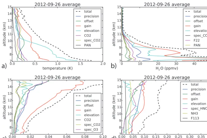
The most important error sources for the primary retrieval targets are depicted in Fig. 4. To mitigate the impact of fil-amentary structures, an averaged error profile is shown. Ob-viously, the remaining uncertainty of elevation angle knowl-edge is the largest contributor to temperature and H2O accu-racy at lower altitudes. Gain and offset are the most impor-tant remaining contributors to accuracy followed by relevant spectroscopic terms and CO2. The error introduced by un-certainty of background CO2VMRs is part of the motivation for the use of WACCM4 data, which capture the general in-crease and also seasonal variations better than the Remedios climatology (Remedios et al., 2007).
The averaging kernels have been diagnosed to provide measurement contribution and vertical resolution (Fig. 5). Due to the nature of the regularisation employed, the mea-surement contribution is very close to 1 over the full alti-tude range, implying that the retrieval results are not biased in absolute value by the regularisation. The vertical resolu-tion is consistently better than 500 m and as low as 250 m close to the aircraft for the trace gases and on the order of 1 km for temperature. The vertical resolution of temperature
P ap er | Discussion P ap er | Discussion P ap er | Disc ussion P ap er | 0 500 1000 1500 2000 0 100 200 300 400500 600 simulation measurement difference 100 10 ra dia nc e ( nW /(c m
2 sr
cm
−
1)
1100 1150 1200 1250 1300 1350 1400
wavenumber (cm−1)
100 10
800 850 wavenumber (cm900 950 −1) 1000 1050
Figure 3.A measured and a simulated dynamics mode spectrum averaged over row 57 (tangent altitude 12.78km) of the detector taken at 14:40:12 (UTC) and 14.45kmaircraft altitude. The spectrum is split at 1090cm−1with the lower panels showing higher wavenumbers. The lines shows the full spectral resolution of the spectra while the markers show the values of the ISWs used in the retrieval. The extent of the ISWs is overlayed as grey bars. The difference plots also contain the target (dots) and threshold (dashes) values for noise. This simulation was performed using the band model. The large discrepancy in the lower panels is caused byN2OandCH4, which are currently not retrieval targets
35
Figure 3. A measured and a simulated dynamics mode spectrum averaged over row 57 (tangent altitude 12.78 km) of the detector taken at 14:40:12 UTC and 14.45 km aircraft altitude. The spec-trum is split at 1090 cm−1with the lower panels showing higher wavenumbers. The lines shows the full spectral resolution of the spectra while the markers show the values of the ISWs used in the retrieval. The extent of the ISWs is overlayed as grey bars. The dif-ference plots also contain the target (dots) and threshold (dashes) values for noise. The vertical red lines separate regions that employ different aerosol/extinction profiles. This simulation was performed using the band model. The large discrepancy in the lower panels is caused by N2O and CH4, which are currently not retrieval targets.
will likely increase, if the CO2Q-branch can be measured to higher precision in the future. The vertical resolution seems to improve again for the lowest altitudes. This is technically correct, but misleading as the shape of the averaging kernels takes on a rather broad base and also partly negative values at lower altitudes. The last two panels of Fig. 5 show the horizontal resolution and displacement. The horizontal reso-lution along the line of sight of retrieved trace gases is on the order of 100 km. The small horizontal displacement for the trace gases asserts that indeed the trace gas VMRs close to the tangent point (the reference point for the displacement) are being retrieved. But the 2-D averaging kernels of temper-ature are shown to be biased towards the instrument location, presumably because the ISWs used to determine the tempature are not optically thin. This discrepancy is another er-ror source introduced by the assumption of horizontal homo-geneity. However, we expect that the effect is mitigated by the application of ECMWF temperature gradients.
2482 J. Ungermann et al.: Level 2 processing for GLORIA dynamics mode
a)
b)
c)
d)
Figure 4. Total error and major error sources for the four primary targets temperature (a), H2O (b), O3(c), and HNO3(d) averaged over the
profiles of the flight of 26 September 2012. A “spec” prefix notes the error induced by spectral uncertainty of line intensities.
b)
a)
d)
c)
Figure 5. Diagnostic quantities for the four primary targets averaged over the profiles of the flight of 26 September 2012: measurement contribution (a), vertical resolution (b), horizontal resolution (c), and horizontal displacement (d). Horizontal resolution and displacement have been computed using the band model; displacement is measured relative to the tangent point location. The resolution is defined as the “full width at half max” of the corresponding row of the averaging kernel matrix.
masses, which were recently mixed from the troposphere into the stratosphere like the filament of comparatively wet air at 12 km around 10:00 UTC.
4.3 Validation
spa-a)
b)
c)
d)
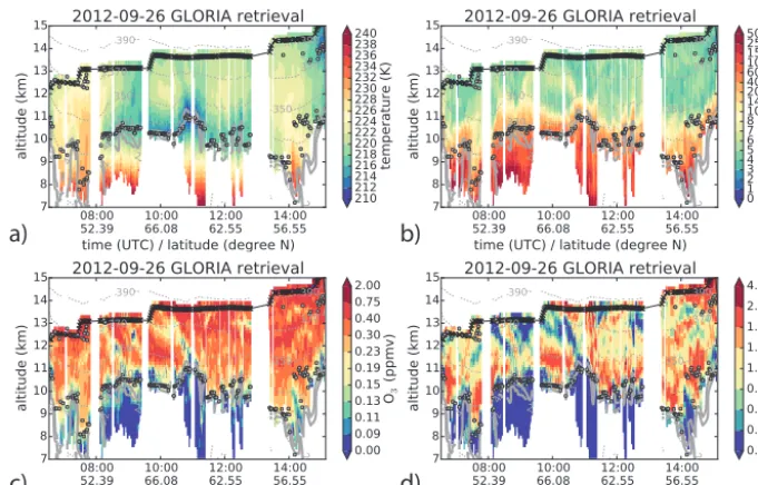
Figure 6. Cross-sections of retrieved quantities for the flight of 26 September 2012: temperature (a), H2O (b), O3(c), and HNO3(d). In
addition, selected isentropes are shown as dotted grey lines, ECMWF potential vorticity (interpolated to the time of measurement) isolines of 2 and 4 PVU are shown as thick grey lines. The thermal tropopause is derived from retrieved temperature profiles and is shown as thick grey dots. Depicted retrieved values are limited below by clouds and above by the flight altitude.
tially and temporally difficult to align. In the given synoptic situation with strong horizontal temperature gradients, also comparing to radiosonde data is difficult due to the sparsity of radiosonde ascents. This leaves the in situ instruments as the best source for validation. Due to the crowded airspace over Oberpfaffenhofen, it was not possible to directly mea-sure with GLORIA the ascent or descent profiles acquired by the in situ instruments. There are measurements of the dive over Norway available, but this situation was selected specif-ically for its large horizontal variability, implying a large sampling uncertainty due to the averaging nature of 1-D re-trievals. The dive will prove valuable for the characterisation of 3-D tomographic retrievals, though, as it is at the centre of a tomographic hexagonal flight pattern.
Comparing the retrieved temperatures (in fact 125 m be-low flight level to mitigate the effect of the top column) against the in situ measurements at flight level is illustrated in Fig. 7. The temperature in Fig. 7a follows closely the measurements, which for this flight agrees also well with ECMWF. Temperatures seem to follow the lower bound of the in situ envelope, which might indicate a low bias (the mean difference is−0.48 K, see Table 5); the most likely ex-planation on the GLORIA side for such a bias would be an imperfection in the calibration of the instrument gain. The correlation of all retrieved values at flight levels for the three processed flights is shown in Fig. 7b. The agreement is within expectation for all flights.
Water vapour agrees within error bars to the FISH mea-surements as shown in Fig. 8a. There seems to be a high bias on the order of 1 ppm (roughly 20 %) after 09:00, which
is according to simulations employing fixed ECMWF tem-peratures related to the low bias in temperature in the same time frame. Another known systematic error source is the use of a standard Voigt line-shape for simulation. Boone et al. (2007) and Schneider et al. (2011) suggest that improved re-sults can be achieved using a speed-dependent Voigt profile. The mean difference for these flights is in the same order but of opposite sign, indicating no consistent systematic prob-lem. The correlation for all processed flights in Fig. 8b shows good agreement. The correlation for the Antarctic flight is lower than for the other flights as the air was very dry and no VMRs above 6 ppm were measured (see also Rolf et al., 2014).
O3 values vary to a much larger degree along the flight path than temperature or H2O. Figure 9a shows that the re-trieval results follow the in situ measurements within given error bars with only few exceptions. These are most likely caused by differences in the measured air masses. Figure 9b shows that the correlation is worse than for temperature and H2O, which may be due to the higher variability of O3 on small spatial scales.
num-2484 J. Ungermann et al.: Level 2 processing for GLORIA dynamics mode Discussion P ap er | Discussion P ap er | Discussion P ap er | Disc ussion P ap er | a) 0 2 4 6 8 10 12 14 16 altitude (km)
2012-09-26
06:00 08:00 10:00 12:00 14:00 16:00 18:00
time (UTC) 210 215 220 225 temperature (K) GLORIA BAHAMAS a priori/ECMWF b)
190 200 210 220 230
GLORIA temperature (K)
190 200 210 220 230
BAHAMAS temperature (K)
2012-09-13 (1.00) 2012-09-23 (0.98) 2012-09-26 (0.91)
Figure 7.Comparison of retrieved temperature 125mbelow flight level and temperature measured by the HALO BAHAMAS system. The error bars of retrieved values use the total error (accuracy plus precision). Panel(a)shows the values over time for the flight of 26 September 2012; in addition the employed a priori information with assumed uncertainty and flight altitude is given. Panel(b)shows the correlation for the three currently processed flights; the Pearson correlation coefficient for the flights is given in the legend. See also Tab. 4.
39
Figure 7. Comparison of retrieved temperature 125 m below flight level and temperature measured by the HALO BAHAMAS system. The error bars of retrieved values use the total error (accuracy plus precision). (a) shows the values over time for the flight of 26 September 2012; in addition the a priori information employed with assumed uncertainty and flight altitude is given. (b) shows the correlation for the three currently processed flights; the Pearson correlation coefficient for the flights is given in the legend. See also Table 5.
Discussion P ap er | Discussion P ap er | Discussion P ap er | Disc ussion P ap er | a) 0 2 4 6 8 10 12 14 16 altitude (km)
2012-09-26
06:00 08:00 10:00 12:00 14:00 16:00 18:00
time (UTC) 1 10 H2 O (p pm v) GLORIA FISH a priori b)
0.5 1 2 5 10 20 50
GLORIA H2O (ppmv)
0.5 1 2 5 10 20 50
FIS
H
H
2O
(p
pm
v)
2012-09-13 (0.59) 2012-09-23 (0.92) 2012-09-26 (0.81)Figure 8.Comparison of retrievedH2O125mbelow flight level andH2Omeasured by FISH. See also Fig. 7 and Tab. 4.
40
Figure 8. Comparison of retrieved H2O 125 m below flight level and H2O measured by FISH. See also Fig. 7 and Table 5.
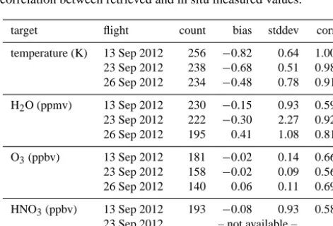
Table 5. Comparison of retrieved targets 125 m below flight level and quantities measured by in situ instruments (BAHAMAS, Fairo, FISH, and AIMS). Shown are the mean difference and the SD. The last column shows the Pearson correlation coefficient for the linear correlation between retrieved and in situ measured values.
target flight count bias stddev corr
temperature (K) 13 Sep 2012 256 −0.82 0.64 1.00 23 Sep 2012 238 −0.68 0.51 0.98 26 Sep 2012 234 −0.48 0.78 0.91
H2O (ppmv) 13 Sep 2012 230 −0.15 0.93 0.59 23 Sep 2012 222 −0.30 2.27 0.92
26 Sep 2012 195 0.41 1.08 0.81
O3(ppbv) 13 Sep 2012 181 −0.02 0.14 0.66
23 Sep 2012 158 −0.02 0.09 0.56
26 Sep 2012 140 0.06 0.11 0.69
HNO3(ppbv) 13 Sep 2012 193 −0.08 0.93 0.58 23 Sep 2012 – not available –
26 Sep 2012 159 0.05 0.40 0.71
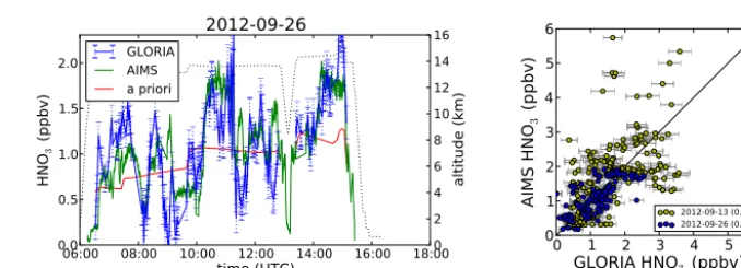
ber of consecutive samples where AIMS measured approxi-mately twice as much HNO3as GLORIA. In the same pro-files, the O3VMR detected by the in situ instrument Fairo is higher than that derived from GLORIA measurements, hence
a very likely explanation is that simply different air masses were measured in the Antarctic polar stratosphere.
The correlation between in situ measurements and GLO-RIA retrieval results is astonishingly low compared to the vi-sual agreement. It is obvious that the GLORIA limb sounder does not measure the radiance emitted at the location of the aircraft, but rather the radiance emitted by an elongated vol-ume around the tangent point. It was found for previous air-craft campaigns that the limb-sounder measurements often lead or lagged behind the in situ measurements as filaments were slanted toward the flight path and were therefore mea-sured earlier or later by the limb sounder than by the in situ instrument (e.g. Ungermann et al., 2012). It is plausible that most anomalies in measured trace gases form elongated fila-ments that are not fully orthogonal to the flight path.
J. Ungermann et al.: Level 2 processing for GLORIA dynamics mode 2485 P ap er | Discussion P ap er | Discussion P ap er | Disc ussion P ap er | a) 0 2 4 6 8 10 12 14 16 altitude (km)
2012-09-26
06:00 08:00 10:00 12:00 14:00 16:00 18:00
time (UTC) 0.0 0.1 0.2 0.3 0.4 0.5 0.6 0.7 O3 (p pm v) GLORIA FAIRO a priori b)
0.0 0.2 0.4 0.6 0.8 1.0 1.2
GLORIA O
3(ppmv)
0.0 0.2 0.4 0.6 0.8 1.0 1.2
FA
IR
O
O
3(p
pm
v)
2012-09-13 (0.66) 2012-09-23 (0.56) 2012-09-26 (0.69)Figure 9.Comparison of retrievedO3125mbelow flight level andO3measured by FAIRO. See also Fig. 7 and Tab. 4.
41
Figure 9. Comparison of retrieved O3125 m below flight level and O3measured by Fairo. See also Fig. 7 and Table 5.
Discussion P ap er | Discussion P ap er | Discussion P ap er | Disc ussion P ap er | a) 0 2 4 6 8 10 12 14 16 altitude (km)
2012-09-26
06:00 08:00 10:00 12:00 14:00 16:00 18:00
time (UTC) 0.0 0.5 1.0 1.5 2.0 HN O3 (p pb v) GLORIA AIMS a priori b)
0 1 2 3 4 5 6
GLORIA HNO3
(ppbv)
0 1 2 3 4 5 6
AI
MS
H
NO
3(p
pb
v)
2012-09-13 (0.58) 2012-09-26 (0.71)Figure 10.Comparison of retrievedHNO3125mbelow flight level andHNO3 measured by AIMS. See also Fig. 7 and Tab. 4. On 23 September 2012, AIMS has been operated in the water vapour mode, therefore noHNO3data are available for that flight.
42
Figure 10. Comparison of retrieved HNO3 125 m below flight level and HNO3 measured by AIMS. See also Fig. 7 and Table 5. On
23 September 2012, AIMS has been operated in the water vapour mode; therefore no HNO3data are available for that flight.
are not subject to such an effect and should deliver more con-sistent results.
5 Conclusions
GLORIA in its present state allows the successful retrieval of several key species and parameters for examining the structure and composition of the highly dynamic UTLS re-gion. The primary targets contain a primarily tropospheric tracer (H2O), a primarily stratospheric tracer (O3), and with a highly resolved temperature product also a quantity to closely examine the thermal tropopause. The vertical reso-lution of 250 to 500 m achieved by GLORIA is a further im-provement over the already highly resolved CRISTA-NF air-borne limb sounder and offers an unprecedented view upon the UTLS. It is expected that the vertical resolution of tem-perature can be further improved when the instrument arte-facts around the CO2 Q-branch have been resolved. The agreement with in situ data is generally good and within range of estimated errors. Discrepancies in correlation can be partially explained by the differences in viewing geome-try and a resulting time-varying lag between the compared instruments.
The results of the last flight on 26 September 2012 demon-strate the Rossby-wave driven intricate structure of the UTLS during summer over Europe that was also observed during
previous campaigns (Ungermann et al., 2013). Future work will expand on this data set by evaluating the remaining TACTS and ESMVal flights after the final level 1 data set is generated for the complete campaign. This paper also pro-vides the basis for the evaluation of upcoming campaigns, which should be even more straightforward due to the in-creased experience with operating the GLORIA instrument.
As has been shown by Kaufmann et al. (2015), one of the major advantages of GLORIA is the capability to use tomographic techniques to create a 3-D reproduction of at-mospheric structure, unaffected by artefacts produced by the assumption of horizontal homogeneity of 1-D retrievals. The current setup provides a sound basis for the tomographic pro-cessing of hexagonal and also linear flight patterns. This will allow exploitation of the full set of GLORIA measurements taken in the dynamics mode.
Acknowledgements. We thank all members of the GLORIA
2486 J. Ungermann et al.: Level 2 processing for GLORIA dynamics mode
providing the WACCM4 model data used in the retrieval. The European Centre for Medium-Range Weather Forecasts (ECMWF) is acknowledged for meteorological data support. The operational implementation of the first tomographic flights was supported by H. Bönisch and A. Engel, who coordinated TACTS. We also gratefully acknowledge the funding of the ESMVal flight hours by DLR and the coordination of ESMVal by H. Schlager. GLORIA retrieval activities were supported under the DFG project RASGLO (HALO-SPP 1294/Ka 2324/1-2) and flight planning by CLaMS model forecasts under the DFG project LASSO (HALO- SPP 1294/GR 3786).
The article processing charges for this open-access publication were covered by a Research
Centre of the Helmholtz Association.
Edited by: C. von Savigny
References
Bange, J., Esposito, M., Lenschow, D. H., Brown, P. R. A., Dreil-ing, V., Giez, A., Mahrt, L., Malinowski, S. P., Rodi, A. R., Shaw, R. A., Siebert, H., Smit, H., and Zöger, M.: Measurement of aircraft state and thermodynamic and dynamic variables, in: Airborne Measurements for Environmental Research: Methods and Instruments, edited by: Wendisch, M., and Brenguier, J.-L., Wiley-VCH Verlag GmbH & Co. KGaA, Weinheim, Germany, 7–75, doi:10.1002/9783527653218.ch2, 2013.
Berthet, G., Esler, J. G., and Haynes, P. H.: A Lagrangian perspective of the tropopause and the ventilation of the lowermost stratosphere, J. Geophys. Res., 112, D18102, doi:10.1029/2006JD008295, 2007.
Birner, T.: Fine-scale structure of the extratropical tropopause region, J. Geophys. Res., 111, D04104, doi:10.1029/2005JD006301, 2006.
Blank, J.: Tomographic Retrieval of Atmospheric Trace Gases Ob-served by GLORIA, Forschungszentrum Jülich, Jülich, PhD the-sis, Wuppertal University, 2013.
Boone, C. D., Walker, K. A., and Bernath, P. F.: Speed-dependent Voigt profile for water vapor in infrared remote sensing applications, J. Quant. Spectrosc. Ra., 105, 525–532, doi:10.1016/j.jqsrt.2006.11.015, 2007.
Chen, P.: Isentropic cross-tropopause mass exchange in the extratropics, J. Geophys. Res., 100, 16661–16673, doi:10.1029/95JD01264, 1995.
Curtis, A. R.: Discussion of “A statistical model for water vapour absorption” by R. M. Goody, Q. J. Roy. Meteor. Soc., 78, 638– 640, 1952.
Dudhia, A., Morris, P. E., and Wells, R. J.: Fast monochromatic ra-diative transfer calculations for limb sounding, J. Quant. Spec-trosc. Ra., 74, 745–756, doi:10.1016/S0022-4073(01)00285-0, 2002.
Fahey, D. W., Gao, R.-S., Möhler, O., Saathoff, H., Schiller, C., Ebert, V., Krämer, M., Peter, T., Amarouche, N., Avallone, L. M., Bauer, R., Bozóki, Z., Christensen, L. E., Davis, S. M., Durry, G., Dyroff, C., Herman, R. L., Hunsmann, S., Khaykin, S. M., Mack-rodt, P., Meyer, J., Smith, J. B., Spelten, N., Troy, R. F., Vömel, H., Wagner, S., and Wienhold, F. G.: The AquaVIT-1
intercom-parison of atmospheric water vapor measurement techniques, At-mos. Meas. Tech., 7, 3177–3213, doi:10.5194/amt-7-3177-2014, 2014.
Fischer, H., Birk, M., Blom, C., Carli, B., Carlotti, M., von Clar-mann, T., Delbouille, L., Dudhia, A., Ehhalt, D., EndeClar-mann, M., Flaud, J. M., Gessner, R., Kleinert, A., Koopman, R., Langen, J., López-Puertas, M., Mosner, P., Nett, H., Oelhaf, H., Perron, G., Remedios, J., Ridolfi, M., Stiller, G., and Zander, R.: MIPAS: an instrument for atmospheric and climate research, Atmos. Chem. Phys., 8, 2151–2188, doi:10.5194/acp-8-2151-2008, 2008. Francis, G. L., Edwards, D. P., Lambert, A., Halvorson, C. M.,
Lee-Taylor, J. M., and Gille, J. C.: Forward modeling and ra-diative transfer for the NASA EOS-Aura High Resolution Dy-namics Limb Sounder (HIRDLS) instrument, J. Geophys. Res., 111, D13301, doi:10.1029/2005JD006270, 2006.
Friedl-Vallon, F., Riese, M., Maucher, G., Lengel, A., Hase, F., Preusse, P., and Spang, R.: Instrument concept and preliminary performance analysis of GLORIA, Adv. Space Res., 37, 2287– 2291, doi:10.1016/j.asr.2005.07.075, 2006.
Friedl-Vallon, F., Gulde, T., Hase, F., Kleinert, A., Kulessa, T., Maucher, G., Neubert, T., Olschewski, F., Piesch, C., Preusse, P., Rongen, H., Sartorius, C., Schneider, H., Schönfeld, A., Tan, V., Bayer, N., Blank, J., Dapp, R., Ebersoldt, A., Fischer, H., Graf, F., Guggenmoser, T., Höpfner, M., Kaufmann, M., Kretschmer, E., Latzko, T., Nordmeyer, H., Oelhaf, H., Orphal, J., Riese, M., Schardt, G., Schillings, J., Sha, M. K., Suminska-Ebersoldt, O., and Ungermann, J.: Instrument concept of the imaging Fourier transform spectrometer GLORIA, Atmos. Meas. Tech., 7, 3565– 3577, doi:10.5194/amt-7-3565-2014, 2014.
Garcia, R. R., Marsh, D., Kinnison, D. E., Boville, B., and Sassi, F.: Simulations of secular trends in the mid-dle atmosphere 1950–2003, J. Geophys. Res., 112, D09301, doi:10.1029/2006JD007485, 2007.
Giez, A.: Effective test and calibration of a trailing cone system on the atmospheric research aircraft HALO, in: Proceedings of the 56th Annual Symposium of the Society of Experimental Test Pilots, Anaheim, USA, 35–46, 2012.
Gille, J. C., Barnett, J., Arter, P., Barker, M., Bernath, P., Boone, C., Cavanaugh, C., Chow, J., Coffey, M., Craft, J., Craig, C., Di-als, M., Dean, V., Eden, T., Edwards, D. P., Francis, G., Halvor-son, C., Harvey, L., Hepplewhite, C., Khosravi, R., KinniHalvor-son, D., Krinsky, C., Lambert, A., Lee, H., Lyjak, L., Loh, J., Mankin, W., Massie, S., McInerney, J., Moorhouse, J., Nardi, B., Pack-man, D., Randall, C., Reburn, J., Rudolf, W., Schwartz, M., Serafin, J., Stone, K., Torpy, B., Walker, K., Waterfall, A., Watkins, R., Whitney, J., Woodard, D., and Young, G.: The high-resolution dynamics limb sounder: experiment overview, recov-ery, and validation of initial temperature data, J. Geophys. Res., 113, D16S43, doi:10.1029/2007JD008824, 2008.
Gille, J., Karol, S., Kinnison, D., Lamarque, J.-F., and Yudin, V.: The role of midlatitude mixing barriers in creating the annual variation of total ozone in high northern latitudes, J. Geophys. Res., 119, 9578–9595, doi:10.1002/2013JD021416, 2014. Glatthor, N., von Clarmann, T., Fischer, H., Funke, B., Grabowski,
(MIPAS), Atmos. Chem. Phys., 7, 2775–2787, doi:10.5194/acp-7-2775-2007, 2007.
Godson, W. L.: The evaluation of infra-red radiative fluxes due to atmospheric water vapour, Q. J. Roy. Meteor. Soc., 79, 367–379, 1953.
Gordley, L. L. and Russell, J. M.: Rapid inversion of limb radiance data using an emissivity growth approximation, Appl. Optics, 20, 807–813, doi:10.1364/AO.20.000807, 1981.
Griessbach, S., Hoffmann, L., Höpfner, M., Riese, M., and Spang, R.: Scattering in infrared radiative transfer: a comparison between the spectrally averaging model JURASSIC and the line-by-line model KOPRA, J. Quant. Spectrosc. Ra., 127, 102–118, doi:10.1016/j.jqsrt.2013.05.004, 2013.
Guggenmoser, T., Blank, J., Kleinert, A., Latzko, T., Ungermann, J., Friedl-Vallon, F., Höpfner, M., Kaufmann, M., Kretschmer, E., Maucher, G., Neubert, T., Oelhaf, H., Preusse, P., Riese, M., Rongen, H., K. Sha, M., Sumin’ska-Ebersoldt, O., and Tan, V.: New calibration noise suppression techniques for the GLORIA limb imager, Atmos. Meas. Tech. Discuss., 7, 12649–12689, doi:10.5194/amtd-7-12649-2014, 2014.
HALO database: available at: https://halo-db.pa.op.dlr.de/, last ac-cess: 1 December 2014.
Hase, F. and Höpfner, M.: Atmospheric ray path modeling for radiative transfer algorithms, Appl. Optics, 38, 3129–3133, doi:10.1364/AO.38.003129, 1999.
Haynes, P. and Shuckburgh, E.: Effective diffusivity as a diagnostic of atmospheric transport: 1. Stratosphere, J. Geophys. Res., 105, 22777–22794, doi:10.1029/2000JD900093, 2000.
Hegglin, M. I., Boone, C. D., Manney, G. L., and Walker, K. A.: A global view of the extratropical tropopause transition layer from Atmospheric Chemistry Experiment Fourier Transform Spec-trometer O3, H2O, and CO, J. Geophys. Res., 114, D00B11, doi:10.1029/2008JD009984, 2009.
Hoffmann, L. and Alexander, M. J.: Retrieval of stratospheric tem-peratures from Atmospheric Infrared Sounder radiance measure-ments for gravity wave studies, J. Geophys. Res., 114, D07105, doi:10.1029/2008JD011241, 2009.
Jurkat, T., Voigt, C., Arnold, F., Schlager, H., Aufmhoff, H., Schmale, J., Schneider, J., Lichtenstern, M., and Dörnbrack, A.: Airborne stratospheric ITCIMS-measurements of SO2, HCl, and HNO3in the aged plume of volcano Kasatochi, J. Geophys. Res., 115, D00L17, doi:10.1029/2010JD013890, 2010.
Jurkat, T., Voigt, C., Kaufmann, S., Zahn, A., Sprenger, A. M., Hoor, P., Bozem, H., Müller, S., Dörnbrack, A., Schlager, H., Bönisch, H., and Engel, A.: A quantitative analysis of strato-spheric HCl, HNO3, and O3 in the tropopause region near the subtropical jet, Geophys. Res. Lett., 41, 3315–3321, doi:10.1002/2013GL059159, 2014.
Kaufmann, M., Blank, J., Friedl-Vallon, F., Gerber, D., Guggen-moser, T., Höpfner, M., Kleinert, A., Sha, M. K., Oelhaf, H., Riese, M., Suminska-Ebersoldt, O., Woiwode, W., Siddans, R., Kerridge, B., Moyna, B., Rea, S., and Oldfield, M.: Technical Assistance for the Deployment of Airborne Limbsounders Dur-ing ESSenCe, Tech. rep., European Space Agency, 2013. Kaufmann, S., Voigt, C., Jeßberger, P., Jurkat, T., Schlager, H.,
Schwarzenboeck, A., Klingebiel, M., and Thornberry, T.: In situ measurements of ice saturation in young contrails, Geophys. Res. Lett., 41, 702–709, doi:10.1002/2013GL058276, 2014.
Kaufmann, M., Blank, J., Guggenmoser, T., Ungermann, J., En-gel, A., Ern, M., Friedl-Vallon, F., Gerber, D., Grooß, J. U., Guenther, G., Höpfner, M., Kleinert, A., Kretschmer, E., Latzko, Th., Maucher, G., Neubert, T., Nordmeyer, H., Oelhaf, H., Olschewski, F., Orphal, J., Preusse, P., Schlager, H., Schneider, H., Schuettemeyer, D., Stroh, F., Suminska-Ebersoldt, O., Vogel, B., M. Volk, C., Woiwode, W., and Riese, M.: Retrieval of three-dimensional small-scale structures in upper-tropospheric/lower-stratospheric composition as measured by GLORIA, Atmos. Meas. Tech., 8, 81–95, doi:10.5194/amt-8-81-2015, 2015. Kleinert, A., Friedl-Vallon, F., Guggenmoser, T., Höpfner, M.,
Neu-bert, T., Ribalda, R., Sha, M. K., Ungermann, J., Blank, J., Eber-soldt, A., Kretschmer, E., Latzko, T., Oelhaf, H., Olschewski, F., and Preusse, P.: Level 0 to 1 processing of the imaging Fourier transform spectrometer GLORIA: generation of radiometrically and spectrally calibrated spectra, Atmos. Meas. Tech., 7, 4167– 4184, doi:10.5194/amt-7-4167-2014, 2014.
Krautstrunk, M. and Giez, A.: The Transition from FAL-CON to HALO era airborne atmospheric research, in: Atmo-spheric Physics, edited by: Schumann, U., Research Topics in Aerospace, Springer Verlag, Berlin, 609–624, doi:10.1007/978-3-642-30183-4_37, 2012.
Kunz, A., Pan, L. L., Konopka, P., Kinnison, D., and Tilmes, S.: Chemical and dynamical discontinuity at the extratropical tropopause based on START08 and WACCM analysis, J. Geo-phys. Res., 116, D24302, doi:10.1029/2011JD016686, 2011. Lamarque, J.-F., Emmons, L. K., Hess, P. G., Kinnison, D. E.,
Tilmes, S., Vitt, F., Heald, C. L., Holland, E. A., Lauritzen, P. H., Neu, J., Orlando, J. J., Rasch, P. J., and Tyndall, G. K.: CAM-chem: description and evaluation of interactive at-mospheric chemistry in the Community Earth System Model, Geosci. Model Dev., 5, 369–411, doi:10.5194/gmd-5-369-2012, 2012.
Lotz, J., Naumann, U., and Ungermann, J.: Hierarchical Algo-rithmic Differentiation – A Case Study, in: Recent Advances in Algorithmic Differentiation, edited by: Forth, S., Hovland, P., Phipps, E., Utke, J., and Walther, A., Lecture Notes in Computational Science and Engineering, Springer, 87, 187–196, doi:10.1007/978-3-642-30023-3_17, 2012.
Marshall, B. T., Gordley, L. L., and Chu, D. A.: BANDPAK: algorithms for modeling broadband transmission and radi-ance, J. Quant. Spectrosc. Ra., 52, 581–599, doi:10.1016/0022-4073(94)90026-4, 1994.
Mlawer, E. J., Payne, V. H., Moncet, J.-L., Delamere, J. S., Al-varado, M. J., and Tobin, D. D.: Development and recent evalua-tion of the MT_CKD model of continuum absorpevalua-tion, Philos. T. Roy. Soc. A, 370, 1–37, doi:10.1098/rsta.2011.0295, 2012. Nakamura, N.: Two-dimensional mixing, edge formation, and
per-meability diagnosed in area coordinates, J. Atmos. Sci., 53, 1524–1537, 1996.
Offermann, D., Grossmann, K.-U., Barthol, P., Knieling, P., Riese, M., and Trant, R.: Cryogenic infrared spectrometers and telescopes for the atmosphere (CRISTA) experiment and mid-dle atmosphere variability, J. Geophys. Res., 104, 16311–16325, doi:10.1029/1998JD100047, 1999.
2488 J. Ungermann et al.: Level 2 processing for GLORIA dynamics mode
Postel, G. A. and Hitchman, M. H.: A climatol-ogy of Rossby wave breaking along the subtropical tropopause, J. Atmos. Sci., 56, 359–373, doi:10.1175/1520-0469(1999)056<0359:ACORWB>2.0.CO;2, 1999.
Remedios, J. J., Leigh, R. J., Waterfall, A. M., Moore, D. P., Sembhi, H., Parkes, I., Greenhough, J., Chipperfield, M.P., and Hauglustaine, D.: MIPAS reference atmospheres and compar-isons to V4.61/V4.62 MIPAS level 2 geophysical data sets, At-mos. Chem. Phys. Discuss., 7, 9973–10017, doi:10.5194/acpd-7-9973-2007, 2007.
Riese, M., Friedl-Vallon, F., Spang, R., Preusse, P., Schiller, C., Hoffmann, L., Konopka, P., Oelhaf, H., von Clarmann, T., and Höpfner, M.: GLObal limb radiance imager for the atmosphere (GLORIA): scientific objectives, Adv. Space Res., 36, 989–995, doi:10.1016/j.asr.2005.04.115, 2005.
Riese, M., Ploeger, F., Rap, A., Vogel, B., Konopka, P., Dameris, M., and Forster, P.: Impact of uncertainties in atmospheric mixing on simulated UTLS composition and related radiative effects, J. Geophys. Res., 117, D16305, doi:10.1029/2012JD017751, 2012. Riese, M., Oelhaf, H., Preusse, P., Blank, J., Ern, M., Friedl-Vallon, F., Fischer, H., Guggenmoser, T., Höpfner, M., Hoor, P., Kauf-mann, M., Orphal, J., Plöger, F., Spang, R., Suminska-Ebersoldt, O., Ungermann, J., Vogel, B., and Woiwode, W.: Gimballed Limb Observer for Radiance Imaging of the Atmosphere (GLO-RIA) scientific objectives, Atmos. Meas. Tech., 7, 1915–1928, doi:10.5194/amt-7-1915-2014, 2014.
Rodgers, C. D.: Inverse Methods for Atmospheric Sounding: The-ory and Practice, Vol. 2 of Series on Atmospheric, Oceanic and Planetary Physics, World Scientific, Singapore, 2000.
Rolf, C., Afchine, A., Bozem, H., Buchholz, B., Ebert, V., Guggen-moser, T., Hoor, P., Konopka, P., Kretschmer, E., Müller, S., Schlager, H., Spelten, N., Sumin’ska-Ebersoldt, O., Unger-mann, J., Zahn, A., and Krämer, M.: Transport of Antarc-tic stratospheric strongly dehydrated air into the troposphere observed during the HALO-ESMVal campaign 2012, Atmos. Chem. Phys. Discuss., 15, 7895–7932, doi:10.5194/acpd-15-7895-2015, 2015.
Rollins, A. W., Thornberry, T. D., Gao, R. S., Smith, J. B., Sayres, D. S., Sargent, M. R., Schiller, C., Kraemer, M., Spelten, N., Hurst, D. F., Jordan, A. F., Hall, E. G., Voemel, H., Diskin, G. S., Podolske, J. R., Christensen, L. E., Rosenlof, K. H., Jensen, E. J., and Fahey, D. W.: Evaluation of UT/LS hygrometer accuracy by intercomparison during the NASA MACPEX mission, J. Geophys. Res., 119, 1915–1935, doi:10.1002/2013JD020817, 2014.
Rothman, L., Gordon, I., Babikov, Y., Barbe, A., Benner, D. C., Bernath, P., Birk, M., Bizzocchi, L., Boudon, V., Brown, L., Campargue, A., Chance, K., Cohen, E., Coudert, L., Devi, V., Drouin, B., Fayt, A., Flaud, J.-M., Gamache, R., Harri-son, J., Hartmann, J.-M., Hill, C., Hodges, J., Jacquemart, D., Jolly, A., Lamouroux, J., Roy, R. L., Li, G., Long, D., Lyulin, O., Mackie, C., Massie, S., Mikhailenko, S., Müller, H., Naumenko, O., Nikitin, A., Orphal, J., Perevalov, V., Per-rin, A., Polovtseva, E., Richard, C., Smith, M., Starikova, E., Sung, K., Tashkun, S., Tennyson, J., Toon, G., Tyuterev, V., and Wagner, G.: The HITRAN2012 molecular spectro-scopic database, J. Quant. Spectrosc. Ra., 130, 4–50, doi:10.1016/j.jqsrt.2013.07.002, HITRAN2012 special is-sue, 2013.
Schiller, C., Kraemer, M., Afchine, A., Spelten, N., and Sitnikov, N.: Ice water content of Arctic, midlatitude, and tropical cirrus, J. Geophys. Res., 113, D24208, doi:10.1029/2008JD010342, 2008.
Schneider, M., Hase, F., and Blumenstock, T.: Water vapour pro-files by ground-based FTIR spectroscopy: study for an optimised retrieval and its validation, Atmos. Chem. Phys., 6, 811–830, doi:10.5194/acp-6-811-2006, 2006.
Schneider, M., Hase, F., Blavier, J.-F., Toon, G. C., and Leblanc, T.: An empirical study on the importance of a speed-dependent Voigt line shape model for tropospheric water vapor pro-file remote sensing, J. Quant. Spectrosc. Ra., 112, 465–474, doi:10.1016/j.jqsrt.2010.09.008, 2011.
Solomon, S., Qin, D., Manning, M., Alley, R., Berntsen, T., Bindoff, N., Chen, Z., Chidthaisong, A., Gregory, J., Hegerl, G., Heimann, M., Hewitson, B., Hoskins, B., Joos, F., Jouzel, J., Kattsov, V., Lohmann, U., Matsuno, T., Molina, M., Nicholls, N., J.Overpeck, Raga, G., Ramaswamy, V., Ren, J., Rusticucci, M., Somerville, R., Stocker, T., Whetton, P., Wood, R. A., and Wratt, D.: Technical summary, in: Climate Change 2007 – The Physical Science Basis. Contribution of Working Group I to the Fourth Assessment Report of the Inter-governmental Panel on Climate Change, Cambridge University Press, Cambridge, United Kingdom and New York, NY, USA, 2007.
Steck, T. and von Clarmann, T.: Constrained profile retrieval ap-plied to the observation mode of the Michelson Interferome-ter for Passive Atmospheric Sounding, Appl. Optics, 40, 3559– 3571, doi:10.1364/AO.40.003559, 2001.
Tikhonov, A. N. and Arsenin, V. Y.: Solutions of Ill-Posed Prob-lems, Winston, Washington DC, USA, 1977.
Ungermann, J.: Improving retrieval quality for airborne limb sounders by horizontal regularisation, Atmos. Meas. Tech., 6, 15–32, doi:10.5194/amt-6-15-2013, 2013.
Ungermann, J., Blank, J., Lotz, J., Leppkes, K., Hoffmann, L., Guggenmoser, T., Kaufmann, M., Preusse, P., Naumann, U., and Riese, M.: A 3-D tomographic retrieval approach with advec-tion compensaadvec-tion for the air-borne limb-imager GLORIA, At-mos. Meas. Tech., 4, 2509–2529, doi:10.5194/amt-4-2509-2011, 2011.
Ungermann, J., Kalicinsky, C., Olschewski, F., Knieling, P., Hoff-mann, L., Blank, J., Woiwode, W., Oelhaf, H., Hösen, E., Volk, C. M., Ulanovsky, A., Ravegnani, F., Weigel, K., Stroh, F., and Riese, M.: CRISTA-NF measurements with unprecedented ver-tical resolution during the RECONCILE aircraft campaign, At-mos. Meas. Tech., 5, 1173–11