https://doi.org/10.5194/amt-10-4965-2017 © Author(s) 2017. This work is distributed under the Creative Commons Attribution 4.0 License.
A new method for estimating UV fluxes at ground level
in cloud-free conditions
William Wandji Nyamsi1,2, Mikko R. A. Pitkänen2,3, Youva Aoun1, Philippe Blanc1, Anu Heikkilä4, Kaisa Lakkala4,5, Germar Bernhard6, Tapani Koskela7, Anders V. Lindfors2, Antti Arola2, and Lucien Wald1
1Mines ParisTech, PSL Research University, Centre Observation, Impacts, Energy, Sophia Antipolis, France 2Finnish Meteorological Institute, Kuopio, Finland
3Department of Applied Physics, University of Eastern Finland, Kuopio, Finland 4Finnish Meteorological Institute, Climate Research, Helsinki, Finland
5Finnish Meteorological Institute, Arctic Research, Sodankylä, Finland 6Biospherical Instruments Inc., San Diego, California, USA
7Independent researcher, Helsinki, Finland
Correspondence:William Wandji Nyamsi ([email protected]) Received: 1 July 2017 – Discussion started: 10 August 2017
Revised: 3 November 2017 – Accepted: 6 November 2017 – Published: 19 December 2017
Abstract. A new method has been developed to estimate the global and direct solar irradiance in the UV-A and UV-B at ground level in cloud-free conditions. It is based on a resampling technique applied to the results of the k -distribution method and the correlated-k approximation of Kato et al. (1999) over the UV band. Its inputs are the aerosol properties and total column ozone that are produced by the Copernicus Atmosphere Monitoring Service (CAMS). The estimates from this new method have been compared to in-stantaneous measurements of global UV irradiances made in cloud-free conditions at five stations at high latitudes in various climates. For the UV-A irradiance, the bias ranges between −0.8 W m−2 (−3 % of the mean of all data) and
−0.2 W m−2 (−1 %). The root mean square error (RMSE) ranges from 1.1 W m−2 (6 %) to 1.9 W m−2 (9 %). The co-efficient of determination R2is greater than 0.98. The bias for UV-B is between−0.04 W m−2(−4 %) and 0.08 W m−2 (+13 %) and the RMSE is 0.1 W m−2 (between 12 and 18 %).R2ranges between 0.97 and 0.99. This work demon-strates the quality of the proposed method combined with the CAMS products. Improvements, especially in the modeling of the reflectivity of the Earth’s surface in the UV region, are necessary prior to its inclusion into an operational tool.
1 Introduction
Ground-based spectroradiometers are one of the means to monitor the intensity of solar UV fluxes. Such measure-ments are rare due to the high costs of the instrumeasure-ments, op-erations and maintenance. To overcome this scarcity, many researchers have looked for proxies and have studied the rela-tionship between UV radiation and the surface downwelling solar radiation integrated from 280 to 2800 nm, called broad-band radiation, since the latter is measured at a greater num-ber of stations or can be estimated at any place from satellite images (Blanc et al., 2011; Lefèvre et al., 2014). Several em-pirical relationships have been published that relate, with the knowledge of the total ozone column (TOC), the broadband irradiance to the erythemal UV (den Outer et al., 2010; Calbó et al., 2005) or the UV-A, UV-B or UV irradiance (Aculinin et al., 2016; Canada et al., 2003; Foyo-Moreno et al., 1998). An alternative way is the use of an appropriate radiative transfer model (RTM) together with accurate inputs describ-ing the state of the atmosphere in cloud-free conditions and the properties of the ground surrounding the instrument, such as libRadtran (Emde et al., 2016; Mayer and Kylling, 2005). A comparison between 1200 measured UV spectra and esti-mates made with a previous version called uvspec – now part of libRadtran – with only ozone and aerosol optical proper-ties as inputs yielded very good performance for simulating the UV irradiance under cloud-free conditions (Mayer et al., 1997). The relative biases ranged between −11 and +2 % for wavelengths between 295 and 400 nm and solar zenithal angles (SZA) up to 80◦. Using measurements from sites in Finland, Norway and Sweden, Lindfors et al. (2007, 2009) showed that erythemal UV and spectral UV irradiances can be accurately modeled using libRadtran and broadband radi-ation, TOC, the total water vapor column from the ERA-40 data set, the surface albedo as estimated from snow depth and the altitude of the location as input.
RTMs are usually computationally expensive; hundreds of spectral calculations are required to compute the UV irradiance in an RTM. Strategies have been built to re-duce the amount of calculations. Among them are the k -distribution method and correlated-kapproximation by Kato et al. (1999). The approach was originally designed for the calculation of the broadband solar irradiance. It consists in calculating the total solar irradiance, i.e., integrated between 240 and 4000 nm, with only 32 spectral calculations in the spectral range between 240 and 4606 nm. The operational McClear model estimating the total irradiance in cloud-free conditions accurately reproduces the irradiance computed by libRadtran based on the Kato et al. (1999) approach (Lefèvre et al., 2013). The McClear model uses several look up ta-bles computed by libRadtran for selected values of inputs and provides the irradiance at each of the 32 spectral intervals. Hereafter, these 32 spectral intervals are named Kato bands and abbreviated KB with the number in subscript. Four KBs cover the whole UV range: KB3 [283, 307] nm, KB4 [307,
328] nm, KB5[328, 363] nm and KB6[363, 408] nm. In KB1
and KB2, atmospheric ozone attenuates the radiation before
it reaches the ground.
Wandji Nyamsi et al. (2014) compared atmospheric trans-missivities obtained by the Kato et al. (1999) approach against those obtained by spectrally resolved computations using two RTMs in each of the 32 KBs. These calculations were performed for a set of 200 000 realistic atmospheres and clouds. As for the UV band, the authors found that the Kato et al. (1999) approach offers very accurate estimates of irradiances in KB5 and KB6. On the contrary, a very
large underestimation of the transmissivity was observed in KB3 [283, 307] nm and KB4[307, 328] nm by respectively
−93 and−16 % in relative value and exhibits a relative root mean square error (RMSE) of 123 and 17 % in clear-sky conditions. Similar relative errors are observed for cloudy conditions. This is due to the assumption made by Kato et al. (1999) that in these bands a single ozone cross section at the central wavelength is sufficient to accurately represent the absorption by ozone over the whole interval. In a sub-sequent work, Wandji Nyamsi et al. (2015b) have proposed a novel parameterization using more than one single ozone cross sections which accurately represents the transmissivity due to ozone absorption. The novel parameterization of the transmissivity using more quadrature points yields maximum errors of respectively 0.0006 and 0.0143 for intervals KB3
and KB4. Version 2.0.1 of libRadtran (Emde et al., 2016)
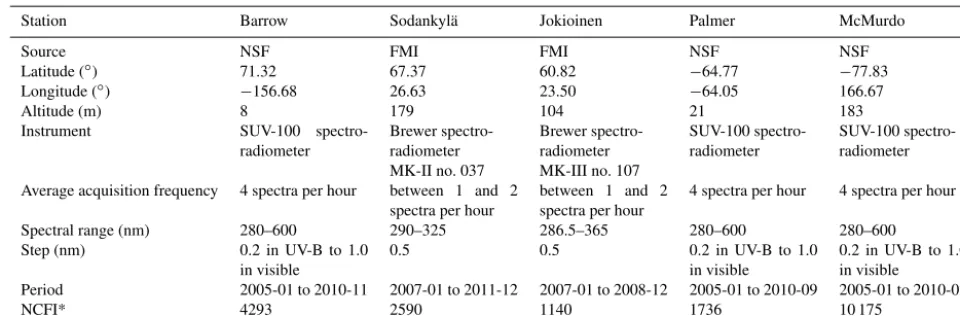
2 Description of measurements used for comparison Ground-based measurements were collected from three sites of the UV network of the National Science Foundation (NSF) of the USA and two sites of the Finnish Meteorological In-stitute (FMI). Table 1 reports the geographical coordinates of the stations, time period of data and their source, type of instruments, spectral interval and step of measurements.
The Barrow site is located approximately 6 km northeast of the Barrow city in Alaska, on the coast of the Chukchi Sea, part of the Arctic Ocean, usually covered by ice be-tween November and July. The snow cover of the surround-ings of the station extends from October until June. Accord-ing to Bernhard et al. (2008), the effective UV albedo of the surface reaches its maximum of approximately 0.8 during March–April. It decreases to 0.05 in summer from August until September.
The Sodankylä site is approximately 6 km south of the vil-lage of Sodankylä. The site is located in the vicinity of the river Kitinen, and the surroundings are boreal pine forest and large peatland areas. A permanent snow cover is present dur-ing the winter and the annual number of snowy days is on average 190. The snow cover starts accumulating in October or November and melts away during May almost every year. The effective UV albedo follows a seasonal variation due to the snow cover. It ranges from very low values in boreal sum-mer up to 0.65 in winter (Arola et al., 2003).
Jokioinen Observatory is located in a fairly flat rural area in the southwest of Finland surrounded by fields of agricul-ture and a boreal forest. The number of snowy days is typi-cally 130. The snow conditions in Jokioinen vary from year to year and also within each winter. At the earliest, snow may appear at the end of October or early November, while it typ-ically melts away in March or April. The effective UV albedo is highly variable; it may rise up to 0.58 in boreal winter but more typical values are 0.2 to 0.5 (Lindfors et al., 2007).
Palmer is situated on Anvers Island, which is on the west-ern side of the Antarctic Peninsula. The ocean surrounding the island is frozen during austral winter and usually ice-free in summer. According to Bernhard et al. (2005), the effective UV albedo varies between 0.6 and 0.95 occurring from Au-gust until November and then decreases down to 0.3 to 0.5 after snowmelt. It is large even in austral summer because of the glaciers surrounding the site.
McMurdo is a coastal site located on Ross Island, a vol-canic island of Antarctica surrounded by a persistence of the ice sheet. The surroundings of the station are mostly made of dark volcanic rocks. McMurdo has an annual cycle of change in effective UV albedo. It ranges between 0.54 (March) and 0.99 (October) (Bernhard et al., 2006).
WMO (2008) reports that uncertainties associated with the measurements in UV by spectrometers are difficult to estimate precisely. Beyond the technical specifics of the site itself, several errors may occur in the calibration of the instrument that include (i) the uncertainties associated
with irradiance transfer standards, (ii) the stability of instru-ments over time and (iii) imperfect directional response. The WMO guide estimates that a 5 % measurement uncertainty at 300 nm can be achieved only under the most rigorous con-ditions at the present time.
The data provided by the NSF are available online and can be downloaded freely. Only data of version 2, which have been corrected for the instruments’ cosine error, have been selected to ensure higher accuracy. Data measured dur-ing clear-sky conditions are flagged (flag “CS”). The number of clear-sky instants is reported in Table 1. Integrated irradi-ances in the UV-A and UV-B range are available and have been downloaded from the website http://uv.biospherical. com/Version2.
The data for the two Finnish sites have been corrected for all known errors following the routine spectral UV data pro-cessing procedure of the FMI (Lakkala et al., 2008; Mäkelä et al., 2016). The irradiance scale of the FMI’s Brewer spec-trophotometers is traceable to that maintained by the Finnish National Standards Laboratory at VTT MIKES Metrology and maintained by a rigorous schedule for measurements of primary standard, secondary standard and working standard lamps (Heikkilä et al., 2016a). In this work, the measured UV spectra were first deconvoluted and then convoluted with a standard triangular slit function with a full width at half max-imum of 1 nm and extrapolated using the SHICrivm software package (http://www.rivm.nl/en/Topics/U/UV_ozone_layer_ and_climate/SHICrivm) (Slaper and Koskela, 1997; Slaper et al., 1995) to cover the full UV spectrum as explained in Heikkilä et al. (2016b). Spectral irradiances are integrated over the UV-B and UV-A. The uncertainties related to the extrapolation are less than 2 and 3 % in the integrated UV-A, for the Jokioinen and Sodankylä Brewers respectively when averaged over daily time window. However, for indi-vidual spectra the uncertainties are estimated to be somewhat higher, up to 5–6 % for Sodankylä Brewer with the highest measured wavelength at 325 nm (H. Slaper, personal com-munication, 2017).
Table 1.Description of stations used for validation, ordered by decreasing latitude.
Station Barrow Sodankylä Jokioinen Palmer McMurdo
Source NSF FMI FMI NSF NSF
Latitude (◦) 71.32 67.37 60.82 −64.77 −77.83
Longitude (◦) −156.68 26.63 23.50 −64.05 166.67
Altitude (m) 8 179 104 21 183
Instrument SUV-100
spectro-radiometer
Brewer spectro-radiometer MK-II no. 037
Brewer spectro-radiometer MK-III no. 107
SUV-100 spectro-radiometer
SUV-100 spectro-radiometer Average acquisition frequency 4 spectra per hour between 1 and 2
spectra per hour
between 1 and 2 spectra per hour
4 spectra per hour 4 spectra per hour
Spectral range (nm) 280–600 290–325 286.5–365 280–600 280–600
Step (nm) 0.2 in UV-B to 1.0
in visible
0.5 0.5 0.2 in UV-B to 1.0
in visible
0.2 in UV-B to 1.0 in visible Period 2005-01 to 2010-11 2007-01 to 2011-12 2007-01 to 2008-12 2005-01 to 2010-09 2005-01 to 2010-02
NCFI* 4293 2590 1140 1736 10 175
* NCFI: number of cloud-free instants.
which may go unnoticed in the broadband range, and that the retained series of cloud-free instants for broadband may comprise cloudy instants for UV. Given the high selectivity of the algorithm of Lefèvre et al. (2013), we believe that such cases are rare and that the conclusions will be unaffected as a whole.
3 Description of the new method
In brief, the method combines the fluxes estimated by li-bRadtran in the four KBs and performs a resampling of these fluxes for retrieving UV fluxes. For all the radiative trans-fer simulations, a plane-parallel atmosphere was assumed and the DISORT 2.0 (discrete ordinate technique) algorithm (Stamnes et al., 2000) with 16 streams was selected to solve the radiative transfer equation because several articles have demonstrated the accuracy of its results when compared to robust and more time-consuming solvers.
3.1 Inputs to libRadtran
In cloud-free conditions, UV irradiance at ground level de-pends mostly on the SZA (θs); the ground albedo; the total
column content of ozone; the vertical profile of ozone, tem-perature, pressure, density and volume mixing ratio for gases as a function of altitude; aerosol optical depth (AOD); the Ångström coefficient; and aerosol type and the elevation of the ground above sea level. As the method shall be used op-erationally, the sources of these inputs have been selected to allow estimation of UV irradiance at any location and any time.
The Copernicus Atmosphere Monitoring Service of the European Commission provides aerosol properties together with physically consistent TOC for any place and any time after 2003. Along with TOC, the AOD at 550 nm, Ångström coefficient and aerosol type are collected from this source of data following exactly the path of the McClear model
(Lefèvre et al., 2013).θs is given by the SG2 algorithm for
the Sun position and angles (Blanc and Wald, 2012). Ground elevation is extracted from the Shuttle Radar Topography Mission database and has been downloaded from the web-site http://srtm.csi.cgiar.org/SELECTION/inputCoord.asp.
un-derestimation in UV albedo, hence in a lesser contribution to diffuse UV irradiance, and therefore in the underestimation of the global UV.
3.2 Resampling technique
Letλbe the wavelength,Gλthe global spectral irradiance at the surface andBλthe direct normal spectral irradiance, i.e., the irradiance received from the direction of the Sun at the surface on a plane normal to the Sun’s rays. The irradiance in a given interval [λ1,λ2] is given by
Gλ1λ2=
λ2
Z
λ1
Gλdλ. (1)
Similar expressions may be obtained for irradiances in UV-A, UV-B, UV or over KBj. For example, the UV irradiance GUVand the direct normal irradianceBUV or the irradiance
GKB4in KB4are given by
GUV=
400
Z
280
Gλdλ, (2)
BUV= 400
Z
280
Bλdλ, (3)
GKB4=
328
Z
307
Gλdλ, (4)
whereλis expressed in nm.
The KBs do not fit the UV spectral ranges exactly. For ex-ample, the UV-B is covered by KB3and a part of KB4. One
solution to estimate the irradiance in a UV interval is the use of weighted sums based on the overlap between KBjand this
interval. Another technique is adopted here whose concept is to determine several 1 nm spectral bands NBi whose
trans-missivities are correlated to those of the KBj and are then
used in a linear interpolation process to compute the UV irra-diance. A similar approach has been used by Wandji Nyamsi et al. (2015a) for the calculation of the photosynthetically ac-tive radiation with better results than a weighted sum.
If one assumes that the optical properties of the atmo-sphere do not change over a given NBi, the integrals of
Eqs. (2)–(4) may be replaced by Riemann sums over NBi.
For example, if λi denotes the central wavelength of NBi, GUVcan be approximated by
GUV=
120
X
i=1
Gλi. (5)
If one defines the clearness index KTias
KTi =
Gλi
Eoicos(2s)
, (6)
where Eoi is the irradiance at the top of atmosphere on a
plane normal to the Sun’s rays for NBi for a given instantt,
Eq. (5) becomes
GUV=cos(2s) 120
X
i=1
EoiKTi. (7)
Similarly, the clearness index KTKBj for KBjis given by
KTKBj =
GKBj
EoKBjcos(2s)
. (8)
The solar spectrum of Gueymard (2004) available in libRad-tran was combined with the algorithm SG2 for computing the Sun position (Blanc and Wald, 2012) to yield Eoiand EoKBj.
For the method presented here, we assume that simple and accurate relations, e.g., affine functions, may be found be-tween each KTKBj and a subset of several KTi, called KTk
hereafter. Then it may be possible to interpolate linearly be-tween KTkto obtain an estimate of KTi for eachλi. By
sum-ming the products of Eoi and these interpolated KTi’s over
a given spectral interval, it is then possible to compute the corresponding irradiance. This is the principle of the resam-pling technique. The set of NBkis selected at the beginning
of the procedure and the same set is used for all processing. The number of NBk should be as small as possible in order
to decrease the amount of calculations but still large enough to allow a good accuracy.
The selection of NBk is empirically determined by means
of libRadtran. The current approach is empirical with no guarantee that the selected set of NBk is the optimum. It
could have been possible to use some mathematical opti-mization tools. This is not a straightforward process as the cost function should take into account that the number of NBk is unknown a priori.
A set of 60 000 clear-sky atmospheric states was built by means of the Monte Carlo technique in order to select NBk.
Each state comprises the nine variables described above, and the value of each variable was randomly selected by taking into account their modeled marginal distribution. The dis-tributions proposed by Lefèvre et al. (2013) and Oumbe et al. (2011) established from observations were adopted here (Table 2). More specially, the uniform distribution is chosen as a model for marginal probability for all variables except AOD, the Ångström exponent coefficient, and total column content of ozone. The chi-square law for AOD, the normal law for the Ångström exponent coefficient, and the beta law for TOC have been selected. The selection of these paramet-ric probability density functions and their corresponding pa-rameters have been empirically determined from the analyses of the observations made in the Aerosol Robotic Network for aerosol properties and from meteorological satellite-based ozone products (Lefèvre et al., 2013).
Table 2.Ranges and statistical distributions of values taken by the cosine of the solar zenith angle, the ground albedo and the 7 variables describing the clear atmosphere.
Variable Value
Cosine of the SZA cos (2s) Uniform between 0 and 89 (degree) for2s
Ground albedoρg Uniform between 0 and 0.9
Elevation of the ground above mean sea level Equiprobable in the set{0,1,2,3}(km)
Total column content of ozone Ozone content is 300×β+200, in Dobson unit. Beta distribution, withA
pa-rameter=2 andBparameter=2, to computeβ
Atmospheric profiles (Air Force Geophysics Laboratory standards)
Equiprobable in the set { midlatitude summer, midlatitude winter, subarctic
summer, subarctic winter, tropical, US standard}
Aerosol optical depth at 550 nm Gamma distribution, with shape parameter=2 and scale parameter=0.13
Ångström exponent coefficient Normal distribution, with mean=1.3 and standard-deviation=0.5
Aerosol type Equiprobable in the set{urban, rural, maritime, tropospheric, desert,
continen-tal, Antarctic}
280 300 320 340 360 380 400
0 0.1 0.2 0.3 0.4 0.5 0.6 0.7 0.8
Wavelength (nm)
Clearness index KT
Kato et al. (1999) approach
Selected node
Proposed technique (1 nm band) Reference (1 nm band)
KTKB6 KTKB5
KTKB4
KTKB3
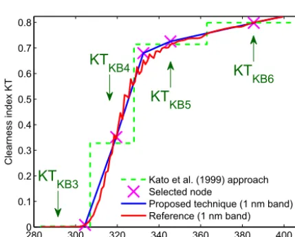
Figure 1.Illustration of the resampling technique.
KTKB4, KTKB5 and KTKB6 and (2) with detailed spectral
computations providing KTievery 1 nm for the interval [283,
408] nm. Several plots were made superimposing KTKB3,
KTKB4, KTKB5 and KTKB6 (in green), and KTi (in red).
Figure 1 is such a graph with the following inputs: θs of
53.76◦, the midlatitude winter atmospheric profile, TOC of 470 DU, AOD of 0.78 at 1000 nm for a maritime polluted aerosol model with an Ångström exponent of 1.93, elevation of 0 m and surface albedo of 0.63. A visual inspection shows that KTKBj and KTi are approximately equal forλj in the
middle of KBj, except for KB5. KTi in this band exhibits a
nonlinear behavior that cannot be accounted for with a single KTk. If one selects 305, 320, 333, 346 and 386 nm as NBk
(magenta crosses), then the linear interpolation (in blue) pro-vides a fairly accurate estimate of KTi. The five NBk’s were
selected by a lengthy visual inspection of such plots and are reported in Table 3. The same NBk’s apply for the global and
direct irradiances. For each NBk, the parameters of the affine
function relating KTKBj and KTk are determined by
least-squares fitting technique (Table 3):
KTk=akKTKBj+bk. (9)
Another set of parameters is determined in the same way for the direct irradiance. In the operational mode, given an atmo-spheric state, a run of libRadtran, or a fast approximation of it, yields four KTKBj, from which the five KTk’s are
com-puted using the affine functions. Then, approximate KT∗i’s are computed for each nm between 280 and 400 nm using a linear interpolation and extrapolation of KTk. In cases where
extrapolation provides negative values, KT∗i is set to 0. Even-tually,GUVis obtained by
GUV=cos(2s) 120
X
i=1
EoiKT∗i. (10)
A similar process is performed for the direct normal irradi-ance BUV as well as for the same quantities in UV-A and
UV-B. As the method provides the spectrum KT∗i, the equa-tion may be extended to include any acequa-tion spectrumS(λ), for example,
GS(λ)=cos(2s)
λ2
X
λ1
EoiS (i)KT∗i. (11)
3.3 Numerical validation
In this section, results of the proposed technique are com-pared with results from the detailed spectral calculations made by libRadtran to assess the accuracy of the proposed technique forGUVA,GUVB,BUVAandBUVB for cloud-free
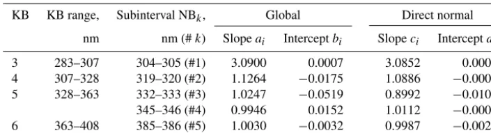
Table 3.KB covering the UV band and selected subintervals NBk; slopes and intercepts of the affine functions between the clearness indices
in KB and subintervals NBk.
KB KB range, Subinterval NBk, Global Direct normal
nm nm (#k) Slopeai Interceptbi Slopeci Interceptdi
3 283–307 304–305 (#1) 3.0900 0.0007 3.0852 0.0003
4 307–328 319–320 (#2) 1.1264 −0.0175 1.0886 −0.0007
5 328–363 332–333 (#3) 1.0247 −0.0519 0.8992 −0.0103
345–346 (#4) 0.9946 0.0152 1.0112 −0.0004
6 363–408 385–386 (#5) 1.0030 −0.0032 0.9987 −0.0023
Table 4.Statistical indicators of the performances of the proposed technique for estimating UV fluxes.
UV Mean Bias RMSE rBias rRMSE R2
fluxes (W m−2) (W m−2) (W m−2) (%) (%)
GUVA 45.6 +0.1 0.1 +0.2 0.2 1.00
BUVA 23.4 −0.1 0.2 −0.6 0.8 1.00
GUVB 2.30 −0.04 0.14 −1.64 6.19 1.00
BUVB 0.73 +0.07 0.15 +10.10 20.48 0.97
compared to the detailed calculations performed by libRad-tran. Following the ISO standard (1995), the deviations were computed by subtracting measurements for each instant from the results of the method. They were summarized by the bias (mean error), the root mean square error, and their values rBias and rRMSE relative to the mean value of the measure-ments. In addition, the coefficient of determination (R2)is computed.
Table 4 reports the statistical indicators for the global and direct normal UV-A and UV-B irradiances. For UV-A fluxes, the bias for the global irradiance and the direct ir-radiance is+0.10 W m−2, i.e.,+0.2 % in relative value, and
−0.15 W m−2, i.e.,−0.7 % in relative value respectively. The RMSE is respectively 0.12 W m−2 (0.3 %) and 0.18 W m−2 (0.8 %). For UV-B fluxes, the bias for the global irradiance and the direct irradiance is −0.04 W m−2, i.e., −1.6 % in relative value, and +0.07 W m−2, i.e.,+10.1 % in relative value respectively. The corresponding RMSE is respectively 0.14 W m−2 (6.2 %) and 0.15 W m−2 (20.5 %). The coeffi-cient of determinationR2is greater than 0.99 except for the direct normal UV-B irradiance which is 0.966. Expectedly, these indicators prove the good level of performance of the proposed technique.
4 Results
The results of the proposed method were compared to mea-surements of UV-A and UV-B irradiances at the surface for cloud-free conditions. Similar statistical indicators as those presented in the previous section are also computed to syn-thetize the errors.
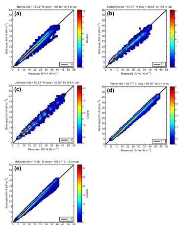
4.1 Performance of the method for UV-A irradiance
Figure 2 exhibits the scatter density plot between ground-based instantaneous measurements made for each station in cloud-free conditions and estimates from the proposed method combined with inputs from CAMS. The station name is indicated at the top of each plot. Figure 2a exhibits the re-sults for Barrow. All points are well located along the identity line. The slope of the fitting line is 0.995, i.e., very close to 1, showing a very good estimation of the measurements by the method.R2is 0.97, meaning that all the variability in the measurements is very well explained by the estimates. The bias is low with a value of−0.2 W m−2, i.e., −1 % of the mean value of the measurements, 20.5 W m−2. The RMSE is small with a value of 1.4 W m−2, which is around 7 % of the mean. These statistical indicators for each station are re-ported in Table 5. The measurements are mostly between March and September. The shortwave albedo is 0.8 from the beginning of March until the middle of May. With the progressive snowmelt, this shortwave albedo decreases from mid-May down to 0.12 in mid-July. This variation corre-sponds well to the climatological evolution reported by Bern-hard et al. (2008) and supports the choice of this approxima-tion by the shortwave albedo.
Even if the points follows the perfect line (Fig. 2a) quite well, a set of points is seen where the method noticeably un-derestimates by more than 20 %. These underestimations oc-curs between the end of May and mid-July. During that pe-riod, the shortwave albedo was less than the effective UV albedo by a factor 0.8. The effective UV albedo is part of the version 2 dataset and was derived by comparing measured clear-sky spectra with corresponding radiative transfer model results (Bernhard et al., 2007). As a smaller albedo means a smaller contribution to the diffuse part of the irradiance, the difference between the shortwave and effective UV albedo may explain these underestimations seen in Fig. 2a.
0 5 10 15 20 25 30 35 40 45 50 55 0
5 10 15 20 25 30 35 40 45 50 55
Measured UV−A (W m−2)
Estimated UV−A (W m
−2)
Barrow (lat = 71.32° N; long = 156.68° W) 8 m asl
(a)
Counts
0 1 2 3 4 5 6 7 8 9 10
1:1
0 5 10 15 20 25 30 35 40 45 50 55 0
5 10 15 20 25 30 35 40 45 50 55
Measured UV−A (W m−2)
Estimated UV−A (W m
−2)
Sodankylä (lat = 67.37° N; long = 26.63° E) 179 m asl
(b)
Counts
0 1 2 3 4 5 6 7 8
1:1
0 5 10 15 20 25 30 35 40 45 50 55 0
5 10 15 20 25 30 35 40 45 50 55
Measured UV−A (W m−2)
Estimated UV−A (W m
−2)
Jokioinen (lat = 60.82° N; long = 23.50° E) 104 m asl
(c)
Counts
0 0.5 1 1.5 2 2.5 3 3.5 4 4.5
1:1
0 5 10 15 20 25 30 35 40 45 50 55 0
5 10 15 20 25 30 35 40 45 50 55
Measured UV−A (W m−2)
Estimated UV−A (W m
−2)
Palmer (lat = 64.77° S; long = 64.05° W) 21 m asl
(d)
Counts
0 0.5 1 1.5 2 2.5 3 3.5 4 4.5 5
1:1
0 5 10 15 20 25 30 35 40 45 50 55 0
5 10 15 20 25 30 35 40 45 50 55
Measured UV−A (W m−2)
Estimated UV−A (W m
−2)
McMurdo (lat = 77.83° S; long = 166.67° E) 183 m asl
(e)
Counts
0 5 10 15 20 25 30
1:1
Figure 2.Scatter density plot between measurements of UV-A and estimates for each station with each station name at the top. The color
bar indicates the number of points in the area within the interval 0.4 W m−2×0.4 W m−2.
Table 5.Statistical indicators of the performances of the method for UV-A irradiance.Nis the number of data points.
Station N Mean Bias RMSE rBias rRMSE R2
(W m−2) (W m−2) (W m−2) (%) (%)
Barrow 4293 20.0 −0.2 1.4 −1.1 6.8 0.98
Sodankylä 2590 20.8 −0.5 1.9 −2.5 9.0 0.98
Jokioinen 1140 22.1 −0.5 1.6 −2.1 7.5 0.98
Palmer 1736 24.9 −0.8 1.2 −3.1 4.9 0.99
0.6 0.8 1 1.2
Esti/meas
Barrow
0 74 1022 1486 1559
Sodankyla
0 219 667 797 770
0.6 0.8 1 1.2
Esti/meas
Jokioinen
48 147 236 353 306
SZA range (°) Palmer
0 216 444 482 530
30–40 40–50 50–60 60–70 70–80 0.6
0.8 1 1.2 1.4
Esti/meas
SZA range (°) McMurdo
0 0 1285 3513 4201
−10 −5 0 5
Esti–meas
Barrow
0 74 1022 1486 1559
Sodankyla
0 219 667 797 770
−10 −5 0 5
Esti–meas
Jokioinen
48 147 236 353 306
SZA range (°) Palmer
0 216 444 482 530
−10 −5 0 5
Esti–meas
SZA range (°) McMurdo
0 0 1285 3513 4201
30–40 40–50 50–60 60–70 70–80
30–40 40–50 50–60 60–70 70–80
30–40 40–50 50–60 60–70 70–80
Figure 3.Dependence of ratio (top) of the estimated (esti) to the measured (meas) UV-A irradiances for each station and the differ-ence between the estimated and measured (bottom) UV-A irradi-ances for each station as a function of SZA range. The red dots indicates the mean; the limits of the boxes are the first, second (me-dian) and third quartiles. The lower whisker is the minimum and the upper one is the maximum. The pink number is the number of data in a single SZA range.
The RMSE is low with a value of 1.9 W m−2(9 %). As for Jokioinen (Fig. 2c), all points are well located along the identity line. R2 is 0.98. The bias is low with a value of
−0.5 W m−2, i.e.,−2 % of the mean value of the
measure-ments, 22.1 W m−2, as well as the RMSE with a value of
1.6 W m−2(8 %).
Results for Palmer are shown in Fig. 2d. One may note that the points are well aligned with low scatter along a straight line whose slope is 0.99 with a slight underestimation by the method. The bias is−0.8 W m−2(−3 % of the mean value of 24.9 W m−2). The RMSE is 1.2 W m−2(5 %).R2is greater than 0.99. Cloud-free conditions occur mostly between
Au-gust and April. The shortwave albedo slightly increases from 0.28 to 0.32 between August and March and then decreases until April up to 0.20. These values are small and close to those of a ground free of snow or ice. The effective UV albedo is usually greater than 0.3 with peaks up to 0.8. This difference between the shortwave and effective UV albedo may explain the slight underestimation indicated in Fig. 5.
Results for McMurdo are shown in Fig. 2e. Cloud-free conditions occur mostly between April and September. The points are aligned along the identity line. R2 is 0.99. The bias is low with a value of−0.3 W m−2(−1 % of the mean value of 21.0 W m−2), as well as the RMSE with a value of 1.2 W m−2(6 %). The shortwave albedo may reach 0.8 and there is no clear discrepancy between the shortwave and ef-fective UV albedo. Nevertheless, the authors believe that the outliers may be explained by a difference in albedo.
The dependence of errors as a function of SZA was in-vestigated. Figure 3 exhibits the ratio (top) and difference (bottom) as function ofθs for each station for UV-A
irradi-ances. For the ratio, the limits of the boxes are close from one quartile to another, meaning a very limited spread of the ratio. The deviations between maximum and minimum are approximately small. The median is similar to the mean. Re-gardless of the number of data (in pink color), the deviations are very close to 1 for all SZA ranges and stations except Sodankylä at highθs. As for the ratio, the similar
observa-tions are also seen in terms of the differences at the bottom of Fig. 3. The difference is very close to 0 for all the SZA ranges. The absolute value of the mean difference shows a tendency to decrease asθsincreases, with the maximum
be-ing reached for lowθs.
The dependence of errors as a function of TOC and albedo was also investigated (not shown). The results have revealed that there is no clear dependence of errors as a function of TOC or albedo for all stations. In addition, the absolute val-ues of the bias (not shown) show a tendency to decrease asθs
increases, with the maximum being reached for lowθs,
ex-cept McMurdo. In the opposite manner, the absolute values of the relative bias show a tendency to increase withθs. This
could be related to the fact that lowθs are reached in
sum-mer, with greater values in UV irradiance and lower values in effective UV albedo.
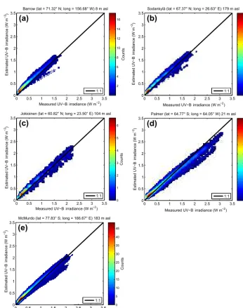
Table 6.Statistical indicators of the performances of the method for UV-B irradiance.Nis the number of data points.
Station N Mean Bias RMSE rBias rRMSE R2
(W m−2) (W m−2) (W m−2) (%) (%)
Barrow 4293 0.57 0.08 0.10 13.41 18.01 0.97
Sodankylä 2590 0.65 0.05 0.09 7.74 13.91 0.98
Jokioinen 1140 0.75 0.05 0.10 6.70 13.74 0.98
Palmer 1736 1.03 −0.04 0.12 −4.24 11.67 0.99
McMurdo 10 175 0.72 0.04 0.09 4.86 12.32 0.98
0 0.5 1 1.5 2 2.5 3 3.5
0 0.5 1 1.5 2 2.5 3 3.5
Measured UV−B irradiance (W m−2)
Estimated UV−B
irradiance (W m
−2)
Barrow (lat = 71.32° N; long = 156.68° W) 8 m asl
(a)
Counts
2 4 6 8 10 12 14 16
1:1
0 0.5 1 1.5 2 2.5 3 3.5
0 0.5 1 1.5 2 2.5 3
3.5 Sodankylä (lat = 67.37° N; long = 26.63° E) 179 m asl
(b)
Counts
0 2 4 6 8 10 12
1:1
0 0.5 1 1.5 2 2.5 3 3.5
0 0.5 1 1.5 2 2.5 3
3.5 Jokioinen (lat = 60.82° N; long = 23.50° E) 104 m asl
(c)
Counts
0 1 2 3 4 5 6
1:1
0 0.5 1 1.5 2 2.5 3 3.5
0 0.5 1 1.5 2 2.5 3
3.5 Palmer (lat = 64.77° S; long = 64.05° W) 21 m asl
(d)
Counts
0 1 2 3 4 5 6 7 8
1:1
0 0.5 1 1.5 2 2.5 3 3.5
0 0.5 1 1.5 2 2.5 3
3.5 McMurdo (lat = 77.83° S; long = 166.67° E) 183 m asl
(e)
Counts
0 5 10 15 20 25 30 35 40 45
1:1
Estimated UV−B
irradiance (W m
−2)
Estimated UV−B
irradiance (W m
−2)
Estimated UV−B
irradiance (W m
−2)
Measured UV−B irradiance (W m−2)
Measured UV−B irradiance (W m−2)
Measured UV−B irradiance (W m−2)
Measured UV−B irradiance (W m−2)
Estimated UV−B
irradiance (W m
−2)
0.5 1 1.5 2
Esti/meas
Barrow
0 74 1022 1486 1559
Sodankyla
0 219 667 797 770
0.5 1 1.5 2
Esti/meas
Jokioinen
48 147 236 353 306
SZA range (°)
Palmer
0 216 444 482 530
0.5 1 1.5 2
Esti/meas
SZA range (°)
McMurdo
0 0 1285 3513 4201
−1
0 1
Esti–meas
Barrow
0 74 1022 1486 1559
Sodankyla
0 219 667 797 770
−1
0 1
Esti–meas
Jokioinen
48 147 236 353 306
SZA range (°)
Palmer
0 216 444 482 530
−1
0 1
Esti–meas
SZA range (°)
McMurdo
0 0 1285 3513 4201 30–40 40–50 50–60 60–70 70–80
30–40 40–50 50–60 60–70 70–80
30–40 40–50 50–60 60–70 70–80
30–40 40–50 50–60 60–70 70–80
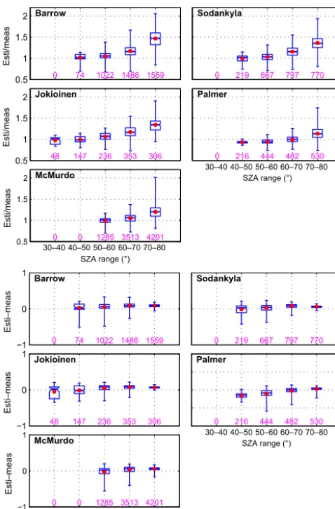
Figure 5.Same as Fig. 3, but for UV-B irradiance.
mostly overestimate when compared to the detailed spectral calculations serving as reference. This observation induces a systematic overestimation at low irradiance from the method. This mainly explains this previous observation. The abso-lute value of the bias is less than 0.1 W m−2. The relative bias ranges between−4 % (Palmer) and 13 % (Barrow). The rRMSE ranges between 12 % and 18 %.
Figure 5 shows the change in ratio and relative difference as a function ofθs. For both ratio and differences, the spread
of limits of the boxes is more or less visible. Nevertheless, the median and the mean are close. The deviations show a tendency to increase withθsfor all stations, probably
mean-ing that a systematic bias from the method is more visible at highθsas mentioned above. These results explained the main
sources of errors for the dependence of errors as a function of TOC and albedo.
In addition, one notices a tendency of the bias to reach a maximum between 65 and 75◦(not shown); this appears in the form of a plateau around 65◦for the RMSE which de-creases asθs increases, i.e., as the irradiance decreases. The
relative bias increases withθsas well as the rRMSE. Both are
closer in the highθsthan in the smallθs.
5 Discussion and conclusion
The comparison has demonstrated a reasonable agreement between the ground-based measurements of UV-A and UV-B and the estimates by the proposed method with CAMS prod-ucts as inputs. The variability in UV fluxes is well reproduced by the method. A good level of accuracy is reached that is close to the uncertainty of the measurements themselves. The computations of the fluxes in the KBs can be performed quite fast with the use of precomputed look up tables as shown by the example of the McClear model. This model is an accu-rate approximation of libRadtran but 105 times faster. The
proposed method extends the results of the McClear model to the UV range and can be used in future operational tools that are both accurate and fast.
Further improvements are needed. A major improvement would be the extension to all sky conditions. In this as-pect, one may build on the work of Oumbe et al. (2014a, b), who demonstrated that, in the case of an infinite plane-parallel single- and double-layered cloud, the solar irradi-ance at ground level computed by a radiative transfer model can be approximated by the product of the irradiance under clear atmosphere and a modification factor that depends on cloud properties and ground albedo only as changes in clear-atmosphere properties have a negligible effect on this factor. Such an approximation has been exploited previously with limited justification by several authors in studies on broad-band irradiance (Huang et al., 2011), UV or photosyntheti-cally active radiation (see e.g., Calbo et al., 2005; den Outer et al., 2010; Krotkov et al., 2001).
Another improvement consists in the modeling of the sur-face albedo in the UV range. Maps of BRDF parameters in the UV range must be created with a satisfactory spatial res-olution of 0.05◦ or better. The MODIS BRDF parameters may be a starting point as they are available at several wave-lengths. It could be possible to apply the technique used by Blanc et al. (2014) to create BRDF maps for each wavelength and for each calendar month with no missing values. The smallest wavelength in the MODIS BRDF is approximately 470 nm, i.e., outside the UV range, and extrapolation towards small wavelengths will be necessary.
Data availability. UV data from Barrow, Palmer station and Mc-Murdo station were provided by the NSF UV Monitoring Net-work operated by Biospherical Instruments Inc. and funded by the US National Science Foundation’s Office of Polar Programs. Ver-sion 2 data used here are available from http://uv.biospherical.com/ Version2/Version2.asp
Products from CAMS can be downloaded from the following website: http://atmosphere.copernicus.eu/
The BRDF maps by Blanc et al. (2014) may be down-loaded from the following website: http://www.oie.mines-paristech. fr/Valorisation/Outils/AlbedoSol/
Competing interests. The authors declare that they have no conflict of interest.
Acknowledgements. William Wandji Nyamsi was partly supported by Fondation Mines ParisTech. We thank Harry Slaper for per-forming studies of uncertainties in SHICrivm.
Edited by: Alexander Kokhanovsky Reviewed by: three anonymous referees
References
Aculinin, A., Brogniez, C., Bengulescu, M., Gillotay, D., Auriol, F., and Wald, L.: Assessment of several empirical relationships for deriving daily means of UV-A irradiance from Meteosat– based estimates of the total irradiance, Remote Sensing, 8, 537, https://doi.org/10.3390/rs8070537, 2016.
Arola, A., Kaurola, J., Koskinen, L., Tanskanen, A., Tikka-nen, T., Taalas, P., and Fioletov, V.: A new approach to estimating the albedo for snow-covered surfaces in the satellite UV method, J. Geophys. Res.-Atmos., 108, https://doi.org/10.1029/2003JD003492, 2003.
Bernhard, G., Booth, C. R., and Ehramjian, J. C.: UV cli-matology at Palmer Station, Antarctica, based on ver-sion 2 NSF network data, Proc. SPIE, 5886, 588607-01, https://doi.org/10.1117/12.614172, 2005.
Bernhard, G., Booth, C. R., Ehramjian, J. C., and Nichol, S. E.: UV climatology at McMurdo station, Antarctica, based on version 2 data of the National Science Foundation’s ultraviolet radiation monitoring network, J. Geophys. Res.-Atmos., 111, 2006. Bernhard, G., Booth, C. R., Ehramjian, J. C., Stone, R. and Dutton,
E. G.: Ultraviolet and visible radiation at Barrow, Alaska: Clima-tology and influencing factors on the basis of version 2 National Science Foundation network data, J. Geophys. Res.-Atmos., 112, D09101, https://doi.org/10.1029/2006JD007865, 2007. Bernhard, G., Booth, C. R., and Ehramjian, J. C.: Comparison of
UV irradiance measurements at Summit, Greenland; Barrow, Alaska; and South Pole, Antarctica, Atmos. Chem. Phys., 8, 4799–4810, https://doi.org/10.5194/acp-8-4799-2008, 2008. Blanc, P. and Wald, L.: The SG2 algorithm for a fast and accurate
computation of the position of the Sun, Sol. Energy, 86, 3072– 3083, https://doi.org/10.1016/j.solener.2012.07.018, 2012. Blanc, P., Gschwind, B., Lefèvre, M., and Wald, L.: The HelioClim
project: Surface solar irradiance data for climate applications, Remote Sensing, 3, 343–361, https://doi.org/10.3390/rs3020343, 2011.
Blanc, P., Gschwind, B., Lefèvre, M., and Wald, L.: Twelve monthly maps of ground albedo parameters derived from MODIS data sets, in: Proceedings of IGARSS 2014, 13–18 July 2014, Que-bec, Canada, USBKey, 3270–3272, available at: http://www.oie.
mines-paristech.fr/Valorisation/Outils/AlbedoSol/ (last access: 1 December 2017), 2014.
Calbó, J., Pages, D., and González, J. A.: Empirical studies of cloud effects on UV radiation: A review, Rev. Geophys., 43, RG2002, https://doi.org/10.1029/2004RG000155, 2005.
Canada, J., Pedros, G., Lopez, A., and Bosca, J. V.: Influences of the clearness index for the whole spectrum and of the relative optical air mass on UV solar irradiance for two locations in the Mediter-ranean area, Valencia and Cordoba, J. Geophys. Res., 105, 4759– 4766, 2003.
Coste, A., Goujon, S., Boniol, M., Marquant, F., Faure, L., Doré, J.-F., Hémon, D., and Clavel, J.: Residential exposure to solar ultraviolet radiation and incidence of childhood hematological malignancies in France, Cancer Cause. Control, 26, 1339–1349, 2015.
de Gruijl, F. R., Sterenborg, H. J., Forbes, P. D., Davies, R. E., Cole, C., Kelfkens, G., van Weelden, H., Slaper, H., and van der Leun, J. C.: Wavelength dependence of skin cancer induction by ultra-violet irradiation of albino hairless mice, Cancer Res., 53, 53–60, 1993.
Delcourt, C., Cougnard-Grégoire, A., Boniol, M., Carrière, I., Doré, F., Delyfer, M.-N. Rougier, M.-B., Le Goff, M., Dartigues, J.-F., Barberger-Gateau, P., and Korobelnik, J. F.: Lifetime exposure to ambient ultraviolet radiation and the risk for cataract extrac-tion and age-related macular degeneraextrac-tion: The Alienor study, Investig. Ophthalmol. Vis. Sci., 55, 7619–7627, 2014.
den Outer, P. N., Slaper, H., Kaurola, J., Lindfors, A., Kazantzidis, A., Bais, A. F., Feister, U., Junk, J., Janouch, M., and Josefsson, W.: Reconstructing of erythemal ultraviolet radiation levels in Europe for the past 4 decades, J. Geophys. Res.-Atmos., 115, D10102, https://doi.org/10.1029/2009JD012827, 2010. Emde, C., Buras-Schnell, R., Kylling, A., Mayer, B., Gasteiger, J.,
Hamann, U., Kylling, J., Richter, B., Pause, C., Dowling, T., and Bugliaro, L.: The libRadtran software package for radia-tive transfer calculations (version 2.0.1), Geosci. Model Dev., 9, 1647–1672, https://doi.org/10.5194/gmd-9-1647-2016, 2016. Fortes, C., Mastroeni, S., Bonamigo, R., Mannooranparampil, T.,
Marino, C., Michelozzi, P., Passarelli, F., and Boniol, M.: Can ultraviolet radiation act as a survival enhancer for cutaneous melanoma?, Eur. J. Cancer Prev., 25, 34–40, 2016.
Foyo-Moreno, I., Vida, J., and Alados-Arboledas, L.: Ground-based ultraviolet (290–385 nm) and broadband solar radiation measure-ments in South-eastern Spain, Int. J. Climatol., 18, 1389–1400, 1998.
Gueymard, C.: The sun’s total and the spectral irradiance for solar energy applications and solar radiations models, Sol. Energy, 76, 423–452, 2004.
Heikkilä, A., Sakari Mäkelä, J., Lakkala, K., Meinander, O., Kaurola, J., Koskela, T., Karhu, J. M., Karppinen, T., Kyrö, E., and de Leeuw, G.: In search of traceability: two decades of calibrated Brewer UV measurements in Sodankylä and Jokioinen, Geosci. Instrum. Method. Data Syst., 5, 531–540, https://doi.org/10.5194/gi-5-531-2016, 2016a.
Herman, J. R. and Celarier, E. A.: Earth surface reflectivity clima-tology at 340 nm to 380 nm from TOMS data, J. Geophys. Res., 102, 28003–28011, 1997.
Huang, G. H., Ma, M. G., Liang, S. L., Liu, S. M., and Li, X.: A LUT-based approach to estimate surface solar irradiance by com-bining MODIS and MTSAT data, J. Geophys. Res.-Atmos., 116, D22201, https://doi.org/10.1029/2011JD016120, 2011. ISO Guide to the Expression of Uncertainty in Measurement: first
edition, International Organization for Standardization, Geneva, Switzerland, 1995.
Juzeniene, A., Brekke, P., Dahlback, A., Andersson-Engels, S., Re-ichrath, J., Moan, K., Holick, M. F., Grant, W. B., and Moan, J.: Solar radiation and human health, Rep. Prog. Phys. 74, 066701, https://doi.org/10.1088/0034-4885/74/6/066701, 2011.
Kato, S., Ackerman, T., Mather, J., and Clothiaux, E.: The k
-distribution method and correlated-k approximation for
short-wave radiative transfer model, J. Quant. Spectrosc. Ra., 62, 109– 121, 1999.
Kravietz, A., Ka, S., Wald, L., Dugravot, A., Singh-Manoux, A., Moisan, F., and Elbaz, A.: Association of UV
ra-diation with Parkinson disease incidence: a
nation-wide French ecologic study, Environ. Res., 154, 50–56, https://doi.org/10.1016/j.envres.2016.12.008, 2017.
Krotkov, N. A., Herman, J. R., Bhartia, P. K., Fioletov, V., and Ah-mad, Z.: Satellite estimation of spectral surface UV irradiance: 2. Effects of homogeneous clouds and snow, J. Geophys. Res.-Atmos., 106, 11743–11759, 2001.
Lakkala, K., Arola, A., Heikkilä, A., Kaurola, J., Koskela, T., Kyrö, E., Lindfors, A., Meinander, O., Tanskanen, A., Gröbner, J., and Hülsen, G.: Quality assurance of the Brewer spectral UV measurements in Finland, Atmos. Chem. Phys., 8, 3369–3383, https://doi.org/10.5194/acp-8-3369-2008, 2008.
Lefèvre, M., Oumbe, A., Blanc, P., Espinar, B., Gschwind, B., Qu, Z., Wald, L., Schroedter-Homscheidt, M., Hoyer-Klick, C., Arola, A., Benedetti, A., Kaiser, J. W., and Morcrette, J.-J.: Mc-Clear: a new model estimating downwelling solar radiation at ground level in clear-sky conditions, Atmos. Meas. Tech., 6, 2403–2418, https://doi.org/10.5194/amt-6-2403-2013, 2013. Lefèvre, M., Blanc, P., Espinar, B., Gschwind, B., Ménard, L.,
Ranchin, T., Wald, L., Saboret, L., Thomas, C., and Wey, E.: The HelioClim-1 database of daily solar radiation at Earth surface: an example of the benefits of GEOSS Data-CORE, IEEE J-STARS, 7, 1745–1753, https://doi.org/10.1109/JSTARS.2013.2283791, 2014.
Lindfors, A., Kaurola, J., Arola, A., Koskela, T., Lakkala, K., Josef-sson, W., Olseth, J. A., and Johnsen, B.: A method for reconstruc-tion of past UV radiareconstruc-tion based on radiative transfer modeling: Applied to four stations in northern Europe, J. Geophys. Res., 112, D23201, https://doi.org/10.1029/2007JD008454, 2007. Lindfors, A., Heikkilä, A., Kaurola, J., Koskela, T., and Lakkala,
K.: Reconstruction of solar spectral surface UV irradiances using radiative transfer simulations, Photochem. Photobiol., 85, 1233– 1239, 2009.
Mäkelä, J. S., Lakkala, K., Koskela, T., Karppinen, T., Karhu, J. M., Savastiouk, V., Suokanerva, H., Kaurola, J., Arola, A., Lindfors, A. V., Meinander, O., de Leeuw, G., and Heikkilä, A.: Data flow of spectral UV measurements at Sodankylä and Jokioinen, Geosci. Instrum. Method. Data Syst., 5, 193–203, https://doi.org/10.5194/gi-5-193-2016, 2016.
Mayer, B. and Kylling, A.: Technical note: The libRadtran soft-ware package for radiative transfer calculations – description and examples of use, Atmos. Chem. Phys., 5, 1855–1877, https://doi.org/10.5194/acp-5-1855-2005, 2005.
Mayer, B., Seckmeyer, G., and Kylling, A.: Systematic long-term comparison of spectral UV measurements and UVSPEC model-ing results, J. Geophys. Res.-Atmos., 102, 8755–8768, 1997. McKinlay, A. F. and Diffey, B. L.: A reference action spectrum for
ultraviolet induced erythema in human skin, The CIE Journal, 6, 17–22, 1987.
Mesrine, S., Kvaskoff, M., Bah, T., Wald, L., Clavel–
Chapelon, F., and Boutron-Ruault, M.-C.: Nevi,
am-bient ultraviolet radiation and thyroid cancer risk: a
French prospective study, Epidemiology, 28, 694–702,
https://doi.org/10.1097/EDE.0000000000000673, 2017. Norval, M.: The effect of ultraviolet radiation on human viral
infec-tions, Photochem. Photobiol., 82, 1495–1504, 2006.
Norval, M. and Halliday, G. M.: The consequences of UV-induced immunosuppression for human health, Photochem. Photobiol., 87, 965–977, https://doi.org/10.1111/j.1751-1097.2011.00969.x, 2011.
Orton, S.-M., Wald, L., Confavreux, C., Vukusic, S., Krohn, J. P., Ramagopalan, S. V., Herrera, B. M., Sadovnick, A. D., and Ebers, G. C.: Association of UV radiation with multiple sclero-sis prevalence and sex ratio in France, Neurology, 76, 425–431, https://doi.org/10.1212/WNL.0b013e31820a0a9f, 2011. Oumbe, A., Blanc, Ph., Gschwind, B., Lefevre, M., Qu, Z.,
Schroedter-Homscheidt, M., and Wald, L.: Solar irradiance in clear atmosphere: study of parameterisations of change with al-titude, Adv. Sci. Res., 6, 199–203, https://doi.org/10.5194/asr-6-199-2011, 2011.
Oumbe, A., Qu, Z., Blanc, P., Lefèvre, M., Wald, L., and Cros, S.: Decoupling the effects of clear atmosphere and clouds to simplify calculations of the broadband solar irra-diance at ground level, Geosci. Model Dev., 7, 1661–1669, https://doi.org/10.5194/gmd-7-1661-2014, 2014a.
Oumbe, A., Qu, Z., Blanc, P., Lefèvre, M., Wald, L., and Cros, S.: Corrigendum to “Decoupling the effects of clear atmo-sphere and clouds to simplify calculations of the broadband solar irradiance at ground level” published in Geosci. Model Dev., 7, 1661–1669, 2014, Geosci. Model Dev., 7, 2409–2409, https://doi.org/10.5194/gmd-7-2409-2014, 2014b.
Schaaf, C. B., Gao, F., Strahler, A. H., Lucht, W., Li, X. W., Tsang, T., Strugnell, N. C., Zhang, X. Y., Jin, Y. F., Muller, J. P., Lewis, P., Barnsley, M., Hobson, P., Disney, M., Roberts, G., Dun-derdale, M., Doll, C., d’Entremont, R. P., Hu, B. X., Liang, S. L., Privette, J. L., and Roy, D.: First operational BRDF, albedo nadir reflectance products from MODIS, Remote Sens. Environ., 83, 135–148, https://doi.org/10.1016/S0034-4257(02)00091-3, 2002.
Setlow, R. B., Grist, E., Thompson, K. and Woodhead, A. D.: Wave-lengths effective in induction of malignant melanoma, P. Natl. Acad. Sci. USA, 90, 6666–6670, 1993.
Kjeldstad, B., Johnson, B., and Koskela, T., Finnish Meteorolog-ical Institute, 89 pp., 1997.
Slaper, H., Reinen, H., Blumthaler, M., Huber, M., and Kuik, F.: Comparing ground-level spectrally resolved solar UV measure-ments using various instrumeasure-ments: A technique resolving effects of wavelength shift and slit width, Geophys. Res. Lett., 22, 2721– 2724, 1995.
Stamnes, K., Tsay, S.-C., Wiscombe, W., and Laszlo, I.: DISORT, a general purpose Fortran program for discrete ordinate method radiative transfer in scattering and emitting layered media: Doc-umentation of methodology, Tech. Rep., Dept. of Physics and Engineering Physics, Stevens Institute of Technology, Hoboken, NJ07030, USA, 2000.
Varotsos, C. A., Melnikova, I. N., Cracknell, A. P., Tzanis, C., and Vasilyev, A. V.: New spectral functions of the near-ground albedo derived from aircraft diffraction spectrometer observations, At-mos. Chem. Phys., 14, 6953–6965, https://doi.org/10.5194/acp-14-6953-2014, 2014.
Wandji Nyamsi, W., Espinar, B., Blanc, P., and Wald, L.: How
close to detailed spectral calculations is the k-distribution
method and correlated-k approximation of Kato et al. (1999)
in each spectral interval?, Meteorol. Z., 23, 547–556,
https://doi.org/10.1127/metz/2014/0607, 2014.
Wandji Nyamsi, W., Espinar, B., Blanc, P., and Wald, L.: Es-timating the photosynthetically active radiation under clear skies by means of a new approach, Adv. Sci. Res., 12, 5–10, https://doi.org/10.5194/asr-12-5-2015, 2015a.
Wandji Nyamsi, W., Arola, A., Blanc, P., Lindfors, A. V., Cesnulyte, V., Pitkänen, M. R. A., and Wald, L.: Technical Note: A novel parameterization of the transmissivity due to ozone absorption
in thek-distribution method and correlated-k approximation of
Kato et al. (1999) over the UV band, Atmos. Chem. Phys., 15, 7449–7456, https://doi.org/10.5194/acp-15-7449-2015, 2015b. WMO: Guide to Meteorological Instruments and Methods of