A multi-model ensemble method that combines imperfect models through learning

(1)

Earth Syst. Dynam., 2, 161–177, 2011 www.earth-syst-dynam.net/2/161/2011/ doi:10.5194/esd-2-161-2011

Earth System

Dynamics

A multi-model ensemble method that combines imperfect models

through learning

L. A. van den Berge1, F. M. Selten1, W. Wiegerinck2, and G. S. Duane3

1_{Royal Netherlands Meteorological Institute, Wilhelminalaan 10, 3732 GK De Bilt, The Netherlands} 2_{Donders Institute for Brain, Cognition and Behaviour, Radboud University Nijmegen, Geert Grooteplein 21,} 6525 EZ Nijmegen, The Netherlands

3_{Department of Atmospheric and Oceanic Sciences, University of Colorado, Boulder, CO 80309, USA} Received: 6 July 2010 – Published in Earth Syst. Dynam. Discuss.: 1 October 2010

Revised: 15 June 2011 – Accepted: 16 June 2011 – Published: 30 June 2011

Abstract. In the current multi-model ensemble approach

cli-mate model simulations are combined a posteriori. In the method of this study the models in the ensemble exchange in-formation during simulations and learn from historical obser-vations to combine their strengths into a best representation of the observed climate. The method is developed and tested in the context of small chaotic dynamical systems, like the Lorenz 63 system. Imperfect models are created by perturb-ing the standard parameter values. Three imperfect models are combined into one super-model, through the introduction of connections between the model equations. The connec-tion coefficients are learned from data from the unperturbed model, that is regarded as the truth.

The main result of this study is that after learning the super-model is a very good approximation to the truth, much better than each imperfect model separately. These illustra-tive examples suggest that the super-modeling approach is a promising strategy to improve weather and climate simula-tions.

1 Introduction

There is a broad scientific consensus that our climate is warming due to anthropogenic emissions of greenhouse gasses (IPCC, 2007). Due to the large impacts of climate change on society there is a growing need to widely sample and assess the possible climate change related to the plausi-ble scenarios for future emissions. At about a dozen climate

Correspondence to: F. M. Selten

([email protected])

institutes around the world complex climate models have been developed over the past decades. Despite the improve-ments in the quality of the model simulations, the models are still far from perfect. For instance a temperature bias of sev-eral degrees in annual mean temperatures in large regions of the globe is not uncommon in the simulations of the present climate (IPCC, 2007).

Nevertheless these models are used to simulate the re-sponse of the climate system to future emission scenarios of greenhouse gasses. It turns out that the models differ substantially in their simulation of the response: the global mean temperature rise varies by as much as a factor of 2 and on regional scales the response can be reversed, e.g. de-creased precipitation instead of an increase. It is not clear how to combine these outcomes to obtain the most realistic response. The standard approach is to take some form of a weighted average of the individual outcomes (Tebaldi and Knutti, 2007), but is this the best strategy?

We think we can do better by letting the models exchange information during the simulation instead of combining the results of the individual models afterwards. We propose to combine the individual models into one super-model by pre-scribing connections between the model equations. The con-nection coefficients are learned from historical observations. This way the super-model learns to combine the strengths of the individual models in order to optimally reproduce the historical climate. Is this approach feasible?

An example of combining models successfully is found in the study by Kirtman et al. (2003) in which they coupled two different atmospheric models to one ocean model. It turned out that the most realistic simulation in terms of the annual mean, annual cycle and interannual variability of sea sur-face temperatures over the tropical pacific was obtained by

(2)

162 L. A. Van den Berge et al.: Combining imperfect models through learning coupling the momentum fluxes from one model and the heat

and fresh water fluxes from the other to the ocean model. Another indication that this approach might be feasible is found in the practice of data assimilation (Compo et al., 2006). It turns out that with a limited amount of informa-tion, the complete state of the atmosphere can be recovered. Synchronization in chaotic systems provides an explanation why this is at all possible, since linking chaotic systems with a signal from one system to the other is known to lead to syn-chronization of their states (Pecora and Carroll, 1990; Duane et al., 2006). Therefore we expect that in the super-modeling approach only limited information needs to be exchanged to effectively influence the combined behaviour of the imper-fect models.

In this paper we use simple chaotic systems to develop and demonstrate the super-modeling approach. We regard the model with standard parameter values as ground truth and create imperfect models by perturbing the parameter values. Three imperfect models are connected and combined into a super-model. The strength of the connections are determined from data from the ground truth through a learning process. The learning process takes the form of the minimisation of a cost function that measures the difference between the truth and the super-model during short integrations.

In Sect. 2 the form of the connections is introduced, fol-lowed by the introduction of the cost function and the min-imisation method. The super-modeling approach is applied to the Lorenz 63, R¨ossler and Lorenz 84 systems in Sects. 3 and 4. Discussion and conclusion of the method and ideas for improvement can be found in Sect. 5.

2 The super-modeling approach

To introduce the super-modeling approach we use the Lorenz 63 system (Lorenz, 1963). The Lorenz 63 system is often used as a metaphore for the atmosphere, because of its abrupt regime changes and unstable nature. The equations for the Lorenz 63 system are

˙

x=σ (y −x)

˙

y=x (ρ −z) −y (1)

˙

z=xy −βz.

The standard parameter values are σ= 10, β=8₃ and

ρ= 28. Numerical solutions are obtained by a fourth order Runge-Kutta time stepping scheme, with a time step of 0.01.

2.1 Connecting imperfect models

Imperfect models are created by taking three copies of the Lorenz 63 system with perturbed parameter values. A super-model is created by the introduction of linear connection terms

˙

xk =σk (yk −xk) + X j6=k

C_kjx xj − xk

˙

yk =xk (ρk −zk) −yk + X j6=k

C_kjy yj −yk (2)

˙

zk =xk yk−βkzk + X j6=k

C_kjz zj−zk

, k = 1,2,3,

wherek indexes the three imperfect models with perturbed parameter values σk, βk andρk andC_kjx, C_kjy and C_kjz are

referred to as connection coefficients.

Each variable of each model is connected to the other two models. This gives two connection coefficients for each of the variables and a total number of 2×3×3 = 18 connec-tion coefficients. These 18 coefficients will be learned from data that sample the truth. The solution of the super-model, denoted by subscript “s”, is taken to be the average of the imperfect models

xs = 1

3 (x1 +x2 +x3)

ys = 1

3 (y1 +y2 +y3) (3)

zs = 1

3 (z1+z2 +z3).

Note that Eqs. (2) define a new dynamical system with three times the number of degrees of freedom. The super-model is not merely a sort of average system. Depending on the connections, it can have a very different dynamics. The super-model has the potential to outperform the ensem-ble averaged simulations of the individual models because it can display richer dynamical behavior. The learning must ensure that the behavior after learning is more realistic.

2.2 Cost function

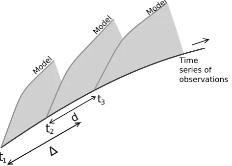
We assume that we have a long time series of observations of the truthxo. We pick initial conditionsxo(ti)from this

long time series atKtimesti,i= 1, ...,K, separated by fixed

distancesd. Short integrations of length 1are performed with the super-model starting from these K initializations (see Fig. 1). To measure the ability of the super-model to follow the truth we introduce the following cost functionF, that depends on the vector of connection coefficientsC.

F (C)= 1

K1

K X

i=1

Z ti+1

ti

|xs(C, t )−xo(t )|2γt dt (4)

The cost function is normalized by _K11 , so that it repre-sents the time averaged mean squared error. The factor γt

with 0< γ≤1 is introduced to give stronger weight to the errors close to the initial conditions. The idea behind this is that the Lorenz 63 system displays sensitive dependence on initial conditions. Trajectories diverge not only due to model imperfections, but also due to internal error growth: even a perfect model deviates from the truth if started from slightly

(3)

L. A. Van den Berge et al.: Combining imperfect models through learning

Van den Berge et al.: Combining imperfect models through learning

163

3

Fig. 1.The cost function is based on short integrations of the super-model starting from observed initial conditions of the truth at times

tiand measures the mean-squared difference between the short

evo-lutions of the super-model and the truth as indicated by the shaded areas. The short integrations span a time interval∆andddenotes the fixed time interval between the initial conditionsti.

model errors, the factor

γ

t

discounts the errors at later times

to decrease the contribution of internal error growth.

We base the choice of

γ

on the doubling time of errors.

From a large number of runs (

10

7

) from randomly perturbed

initial conditions we estimate the average doubling time

τ

of the initial error. We choose

γ

such that

γ

τ

=

1₂

, so at

time

τ

the weight is reduced to

1₂

. For the Lorenz 63

sys-tem

τ

= 0

.

75

, which gives

γ

= 0

.

4

. The length of the short

integrations is taken to be

∆ = 1

, which is a little bit longer

than the doubling time. By comparison the average time for

one rotation in the Lorenz 63 system is 0.8. The separation

d

between the initializations is 0.2 time units.

2.3

Minimisation

For a fixed choice of the number of initializations

K

the cost

function solely depends on the connection coefficients

C

in

equation (4). The super-model can be determined by finding

a minimum in the cost function in the 18 dimensional space

of

C

. For this we employ the Fletcher-Reeves-Polak-Ribiere

Conjugate Gradient method (Fletcher and Reeves, 1963). It

uses the gradient of the cost function to approach minima and

stops when the gradient is (close to) zero.

We found it advantageous to make use of the dependence

of the cost function on the number of initializations

K

to

avoid shallow local minima. We minimize the cost function

first for a small number of initializations. Subsequently we

take this solution as the initial guess of the minimum for an

increased number of initializations to find the minimum for

this set. This process is repeated until we found that the

min-imum did not change any longer by increasing the number of

initializations. This issue is discussed further in section 3.

To avoid negative solutions for the connection coefficients

we added an extra term in the cost function in case one of

σ ρ β

Truth 10 28 8₃

Model 1 13.25 (32%) 19 (32%) 3.5 (31%)

Model 2 7 (30%) 18 (36%) 3.7 (39%)

Model 3 6.5 (35%) 38 (36%) 1.7 (36%)

Table 1.Standard and perturbed parameters for the Lorenz 63 sys-tem.

the coefficients becomes negative. This term is just the

abso-lute value of the negative connection coefficient, which easily

dominates the value of the cost function.

3

Results Lorenz 63

Three imperfect models are created by perturbing the

stan-dard parameter values as displayed in table 1. The perturbed

values differ from the standard values by 30% to 40% and in

each imperfect model parameter values have been increased

as well as decreased. With these perturbations the

imper-fect models behave quite differently from the truth as can be

seen in figure 2. Both model 1 and 2 are attracted to a point,

whereas model 3 has a chaotic solution that resembles the

truth, but the attractor is displaced and larger. All models

were initiated from the same state and the transient evolution

towards the attractor is plotted as well.

By using bifurcation methods, it can be analytically shown

that there exists a Hopf bifurcation for the Lorenz 63 system

at

ρ

H

=

σ(3+_σ₋₁σ₋+_ββ)

. This bifurcation marks different kinds of

dynamical behaviour. Both model 1 and 2 have values for

ρ

below the Hopf bifurcation, whereas model 3 has a value for

ρ

that lies far above the Hopf bifurcation. For the truth the

value of

ρ

lies above the Hopf bifurcation as well, which is

why model 3 and the truth have similar behaviour.

The minimization procedure outlined above successfully

identified a minimum of the cost function with a value of

0.02. By comparison the value of the cost function for an

ar-bitrary choice of all connection coefficients equal to unity

is 0.5. With the connection coefficients of this minimum

we performed a long integration with the super-model and

plotted the trajectory in figure 3. The attractor of the

super-model is very close to the true attractor. While integrating

the super-model, the imperfect models fall into an

approx-imate synchronous behaviour due to the connections: the

temporal correlations between the

x

,

y

, and

z

variables of

the three models are in excess of

0

.

95

(not shown) and the

sum of the time-mean distances between the three model

states normalized by the sum of the standard deviations of

x

s

,

y

s

and

z

s

is 0.34. In particular the

z

-values of the third

model are systematically larger than those of the other two

models (see figure 4). The improvement in the behaviour of

the connected imperfect model solutions as depicted in

fig-ure 4 (to be compared with figfig-ure 2) is a clear indication of

Fig. 1. The cost function is based on short integrations of the

super-model starting from observed initial conditions of the truth at times tiand measures the mean-squared difference between the short evo-lutions of the super-model and the truth as indicated by the shaded areas. The short integrations span a time interval1andddenotes the fixed time interval between the initial conditionsti.

different initial conditions and leads to a non-zero cost func-tion due to chaos. This implies that the cost funcfunc-tion mea-sures a mixture of model errors and internal error growth. Model errors dominate the inital divergence between model and truth, but at later times in the short term integrations in-ternal error growth dominates. Since we wish to measure the model errors, the factorγt discounts the errors at later times to decrease the contribution of internal error growth.

We base the choice ofγ on the doubling time of errors. From a large number of runs (107) from randomly perturbed initial conditions we estimate the average doubling timeτ of the initial error. We chooseγ such thatγτ=1₂, so at time

τ the weight is reduced to 1₂. For the Lorenz 63 system

τ= 0.75, which gives γ= 0.4. The length of the short inte-grations is taken to be1= 1, which is a little bit longer than the doubling time. By comparison the average time for one rotation in the Lorenz 63 system is 0.8. The separation d

between the initializations is 0.2 time units.

2.3 Minimisation

For a fixed choice of the number of initializationsKthe cost function solely depends on the connection coefficientsC in Eq. (4). The super-model can be determined by finding a minimum in the cost function in the 18 dimensional space ofC. For this we employ the Fletcher-Reeves-Polak-Ribiere Conjugate Gradient method (Fletcher and Reeves, 1963). It uses the gradient of the cost function to approach minima and stops when the gradient is (close to) zero.

We found it advantageous to make use of the dependence of the cost function on the number of initializations K to avoid shallow local minima. We minimize the cost function

Table 1. Standard and perturbed parameters for the Lorenz 63

system.

σ ρ β

Truth 10 28 8₃

Model 1 13.25 (32 %) 19 (32 %) 3.5 (31 %) Model 2 7 (30 %) 18 (36 %) 3.7 (39 %) Model 3 6.5 (35 %) 38 (36 %) 1.7 (36 %)

first for a small number of initializations. Subsequently we take this solution as the initial guess of the minimum for an increased number of initializations to find the minimum for this set. This process is repeated until we found that the min-imum did not change any longer by increasing the number of initializations. This issue is discussed further in Sect. 3.

To avoid negative solutions for the connection coefficients we added an extra term in the cost function in case one of the coefficients becomes negative. This term is just the abso-lute value of the negative connection coefficient, which easily dominates the value of the cost function.

3 Results Lorenz 63

Three imperfect models are created by perturbing the stan-dard parameter values as displayed in Table 1. The perturbed values differ from the standard values by 30 % to 40 % and in each imperfect model parameter values have been increased as well as decreased. With these perturbations the imperfect models behave quite differently from the truth as can be seen in Fig. 2. Both model 1 and 2 are attracted to a point, whereas model 3 has a chaotic solution that resembles the truth, but the attractor is displaced and larger. All models were initi-ated from the same state and the transient evolution towards the attractor is plotted as well.

By using bifurcation methods, it can be analytically shown that there exists a Hopf bifurcation for the Lorenz 63 system atρH=σ (_σ3−+1σ−+ββ). This bifurcation marks different kinds of

dynamical behaviour. Both model 1 and 2 have values forρ

below the Hopf bifurcation, whereas model 3 has a value for

ρ that lies far above the Hopf bifurcation. For the truth the value ofρ lies above the Hopf bifurcation as well, which is why model 3 and the truth have similar behaviour.

The minimisation procedure outlined above successfully identified a minimum of the cost function with a value of 0.02. By comparison the value of the cost function for an arbitrary choice of all connection coefficients equal to unity is 0.5. With the connection coefficients of this minimum we performed a long integration with the super-model and plotted the trajectory in Fig. 3. The attractor of the super-model is very close to the true attractor. While integrating the super-model, the imperfect models fall into an approx-imate synchronous behaviour due to the connections: the

(4)

164 L. A. Van den Berge et al.: Combining imperfect models through learning

4

Van den Berge et al.: Combining imperfect models through learning

x y 10 20 30 40 50 60 70 z Truth Model 1 -20 -15 -10 -5 0 5 10 15

20 -40-30-20-10 0 10 20 30

z

(a) Model 1

x y 10 20 30 40 50 60 70 z Truth Model 2 -20 -15 -10 -5 0 5 10 15

20 -40-30-20-10 0 10 20 30

z

(b) Model 2

x y 0 10 20 30 40 50 60 70 z Truth Model 3 -20 -15 -10 -5 0 5 10 15

20 -40-30-20-10 0 10 20 30

z

(c) Model 3

Fig. 2.

Trajectories for the three unconnected imperfect models

(black) and the standard Lorenz 63 system (grey). The trajectory

for the imperfect models includes the transient evolution from the

initial condition towards the attractor.

the feasibility of super-modeling in the context of this

low-dimensional chaotic system.

In addition to this minimum, we found that by choosing

different initial values for the connection coefficients in the

minimization procedure different local minima in the cost

function are obtained with values of the cost function that are

of comparable magnitude. In the remainder of this section we

will test the robustness of the learning process, research the

issue of local minima and develop measures to determine the

quality of the different super-model solutions.

3.1

Robustness

The minimum of the cost function is determined on a limited

period of observations of length

(

K

−

1)

·

d

+ ∆

that we refer

to as the training set. We have chosen

K

= 200

to determine

the minimum and subsequently evaluate the cost function

us-ing the

C

values of this minimum for subsets of the training

set of length corresponding to

K

= 20

,

50

,

100

,

150

. Cross

sections of the cost function around the minimum can be

cre-ated by changing one connection coefficient and keeping the

others fixed at the values of the minimum. The cross sections

-20 -15 -10 -5 0 5 10 15 20 -30 -20 -10 0 10 20 30 0 10 20 30 40 50 z

Lorenz 63 (connected, after learning)

Truth Super-model

x

y z

(a) Point of view 1

x y 0 10 20 30 40 50 z

Truth Super-model -20 -15 -10 -5 0 5 10 15

20 -30-20-10 0 10 20 30

z

(b) Point of view 2

Fig. 3.

Trajectories for the super-model (black) and the standard

Lorenz 63 system (grey) from two different points of view.

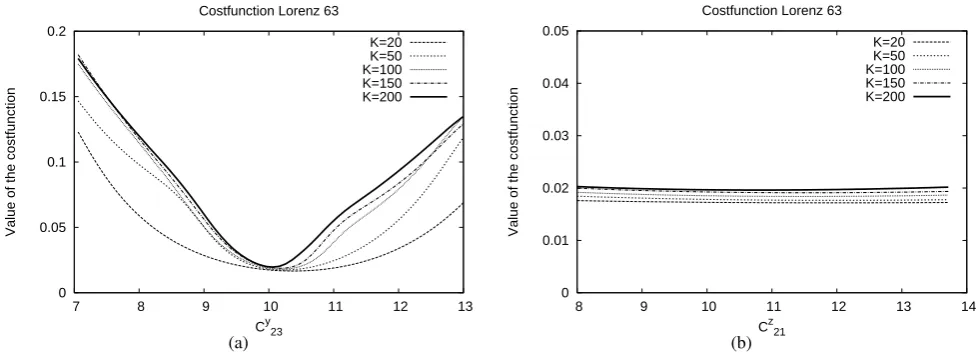
for the different subsets are plotted in figure 5 for connection

coefficients

C

₂₃y

and

C

₂₁z

, since these are typical examples.

In figure 5(a) the cost function for

K

= 200

displays one

well defined minimum

C

₂₃y

= 10

.

1

. The position of the

min-imum does not change much when the cost function is

cal-culated using the different subsets. The minimum becomes

more pronounced as the training set is enlarged. The values

of the cost function monotonically converge and

K

= 200

seems a reasonable size of the training set. Figure 5(b) does

not show a well defined minimum for any

K

. Note that the

scale is smaller than in figure 5(a). The values of the cost

function do not change much in the different subsets and the

slopes are very flat. Changing connection coefficient

C

₂₁z

ap-parently does not change the quality of the solutions much.

A family of super-models of similar quality can be found by

changing connection coefficient

C

₂₁z

between 8 and 14.

Ideally the super-model found by the learning process is

not dependent on the training set. To test whether

K

= 200

is large enough for this to be true the cost function is plotted

in figure 6 for different periods of observations: the training

set and independent sets of the same size that were obtained

from a longer consecutive integration of the truth. Again the

cross sections for connection coefficients

C

₂₃y

and

C

₂₁z

are

shown (figure 6). In figure 6(a) the position and value of the

minimum remain close to that of the training set. In figure

6(b) the cost function is flat for all sets of observations. We

conclude that with

K

= 200

the cost function verifies rather

well on independent data, so

K

= 200

seems a reasonable

4

Van den Berge et al.: Combining imperfect models through learning

x y 10 20 30 40 50 60 70 z Truth Model 1 -20 -15 -10 -5 0 5 10 15

20 -40-30-20-10 0 10 20 30

z

(a) Model 1

x y 10 20 30 40 50 60 70 z Truth Model 2 -20 -15 -10 -5 0 5 10 15

20 -40-30-20-10 0 10 20 30

z

(b) Model 2

x y 0 10 20 30 40 50 60 70 z Truth Model 3 -20 -15 -10 -5 0 5 10 15

20 -40-30-20-10 0 10 20 30

z

(c) Model 3

Fig. 2.

initial condition towards the attractor.

the feasibility of super-modeling in the context of this

of comparable magnitude. In the remainder of this section we

3.1

Robustness

(

K

−

1)

·

d

+ ∆

that we refer

K

= 200

to determine

us-ing the

C

K

= 20

,

50

,

100

,

150

. Cross

cre-ated by changing one connection coefficient and keeping the

-20 -15 -10 -5 0 5 10 15 20 -30 -20 -10 0 10 20 30 0 10 20 30 40 50 z

Truth Super-model

x

y z

(a) Point of view 1

x y 0 10 20 30 40 50 z

20 -30-20-10 0 10 20 30

z

(b) Point of view 2

Fig. 3.

for the different subsets are plotted in figure 5 for connection

coefficients

C

₂₃y

and

C

₂₁z

K

= 200

displays one

C

₂₃y

= 10

.

1

more pronounced as the training set is enlarged. The values

K

= 200

K

. Note that the

function do not change much in the different subsets and the

C

₂₁z

C

₂₁z

between 8 and 14.

not dependent on the training set. To test whether

K

= 200

cross sections for connection coefficients

C

₂₃y

and

C

₂₁z

are

conclude that with

K

= 200

well on independent data, so

K

= 200

seems a reasonable

4

x y 10 20 30 40 50 60 70 z Truth Model 1 -20 -15 -10 -5 0 5 10 15

20 -40-30-20-10 0 10 20 30

z

(a) Model 1

x y 10 20 30 40 50 60 70 z Truth Model 2 -20 -15 -10 -5 0 5 10 15

20 -40-30-20-10 0 10 20 30

z

(b) Model 2

x y 0 10 20 30 40 50 60 70 z Truth Model 3 -20 -15 -10 -5 0 5 10 15

20 -40-30-20-10 0 10 20 30

z

(c) Model 3

Fig. 2.

initial condition towards the attractor.

of comparable magnitude. In the remainder of this section we

3.1

Robustness

(

K

−

1)

·

d

+ ∆

that we refer

K

= 200

to determine

us-ing the

C

K

= 20

,

50

,

100

,

150

. Cross

cre-ated by changing one connection coefficient and keeping the

-20 -15 -10 -5 0 5 10 15 20 -30 -20 -10 0 10 20 30 0 10 20 30 40 50 z

Truth Super-model

x

y z

(a) Point of view 1

x y 0 10 20 30 40 50 z

20 -30-20-10 0 10 20 30

z

(b) Point of view 2

Fig. 3.

for the different subsets are plotted in figure 5 for connection

coefficients

C

₂₃y

and

C

₂₁z

K

= 200

displays one

C

₂₃y

= 10

.

1

more pronounced as the training set is enlarged. The values

K

= 200

K

. Note that the

function do not change much in the different subsets and the

C

₂₁z

C

₂₁z

between 8 and 14.

not dependent on the training set. To test whether

K

= 200

cross sections for connection coefficients

C

₂₃y

and

C

₂₁z

are

conclude that with

K

= 200

well on independent data, so

K

= 200

seems a reasonable

Fig. 2. Trajectories for the three unconnected imperfect models

(black) and the standard Lorenz 63 system (grey). The trajectory for the imperfect models includes the transient evolution from the initial condition towards the attractor.

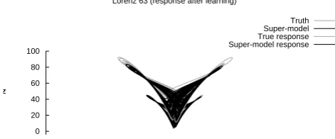
temporal correlations between thex,y, andzvariables of the three models are in excess of 0.95 (not shown) and the sum of the time-mean distances between the three model states normalized by the sum of the standard deviations ofxs, ys andzs is 0.34. In particular thez-values of the third model are systematically larger than those of the other two models (see Fig. 4). The improvement in the behaviour of the con-nected imperfect model solutions as depicted in Fig. 4 (to be compared with Fig. 2) is a clear indication of the feasibil-ity of super-modeling in the context of this low-dimensional chaotic system.

In addition to this minimum, we found that by choosing different initial values for the connection coefficients in the minimisation procedure different local minima in the cost function are obtained with values of the cost function that are of comparable magnitude. In the remainder of this section we will test the robustness of the learning process, research the issue of local minima and develop measures to determine the quality of the different super-model solutions.

4

Van den Berge et al.: Combining imperfect models through learning

x y 10 20 30 40 50 60 70 z Truth Model 1 -20 -15 -10 -5 0 5 10 15

20 -40-30-20-10 0 10 20 30 z

(a) Model 1

x y 10 20 30 40 50 60 70 z Truth Model 2 -20 -15 -10 -5 0 5 10 15

20 -40-30-20-10 0 10 20 30 z

(b) Model 2

x y 0 10 20 30 40 50 60 70 z Truth Model 3 -20 -15 -10 -5 0 5 10 15

20 -40-30-20-10 0 10 20 30 z

(c) Model 3

Fig. 2.

initial condition towards the attractor.

the feasibility of super-modeling in the context of this

of comparable magnitude. In the remainder of this section we

3.1

Robustness

(

K

−

1)

·

d

+ ∆

that we refer

K

= 200

to determine

us-ing the

C

K

= 20

,

50

,

100

,

150

. Cross

cre-ated by changing one connection coefficient and keeping the

-20 -15 -10 -5 0 5 10 15 20 -30 -20 -10 0 10 20 30 0 10 20 30 40 50 z

Lorenz 63 (connected, after learning) Truth Super-model

x

y z

(a) Point of view 1

x y 0 10 20 30 40 50 z

20 -30-20-10 0 10 20 30 z

(b) Point of view 2

Fig. 3.

for the different subsets are plotted in figure 5 for connection

coefficients

C

₂₃y

and

C

₂₁z

K

= 200

displays one

C

₂₃y

= 10

.

1

more pronounced as the training set is enlarged. The values

K

= 200

K

. Note that the

function do not change much in the different subsets and the

C

₂₁z

C

₂₁z

between 8 and 14.

not dependent on the training set. To test whether

K

= 200

cross sections for connection coefficients

C

₂₃y

and

C

₂₁z

are

conclude that with

K

= 200

well on independent data, so

K

= 200

seems a reasonable

4

x y 10 20 30 40 50 60 70 z Truth Model 1 -20 -15 -10 -5 0 5 10 15

20 -40-30-20-10 0 10 20 30 z

(a) Model 1

x y 10 20 30 40 50 60 70 z Truth Model 2 -20 -15 -10 -5 0 5 10 15

20 -40-30-20-10 0 10 20 30 z

(b) Model 2

x y 0 10 20 30 40 50 60 70 z Truth Model 3 -20 -15 -10 -5 0 5 10 15

20 -40-30-20-10 0 10 20 30 z

(c) Model 3

Fig. 2.

initial condition towards the attractor.

of comparable magnitude. In the remainder of this section we

3.1

Robustness

(

K

−

1)

·

d

+ ∆

that we refer

K

= 200

to determine

us-ing the

C

K

= 20

,

50

,

100

,

150

. Cross

cre-ated by changing one connection coefficient and keeping the

-20 -15 -10 -5 0 5 10 15 20 -30 -20 -10 0 10 20 30 0 10 20 30 40 50 z

Truth Super-model

x

y z

(a) Point of view 1

x y 0 10 20 30 40 50 z

20 -30-20-10 0 10 20 30 z

(b) Point of view 2

Fig. 3.

for the different subsets are plotted in figure 5 for connection

coefficients

C

23

y

and

C

21

z

K

= 200

displays one

C

23

y

= 10

.

1

more pronounced as the training set is enlarged. The values

K

= 200

K

. Note that the

function do not change much in the different subsets and the

C

21

z

C

21

z

between 8 and 14.

not dependent on the training set. To test whether

K

= 200

cross sections for connection coefficients

C

23

y

and

C

21

z

are

conclude that with

K

= 200

well on independent data, so

K

= 200

seems a reasonable

Fig. 3. Trajectories for the super-model (black) and the standard

3.1 Robustness

The minimum of the cost function is determined on a limited period of observations of length(K−1)·d+1that we refer to as the training set. We have chosenK= 200 to determine the minimum and subsequently evaluate the cost function us-ing theCvalues of this minimum for subsets of the training set of length corresponding toK= 20, 50, 100, 150. Cross sections of the cost function around the minimum can be cre-ated by changing one connection coefficient and keeping the others fixed at the values of the minimum. The cross sections for the different subsets are plotted in Fig. 5 for connection coefficientsC₂₃y andC₂₁z , since these are typical examples.

In Fig. 5a the cost function forK= 200 displays one well defined minimumC₂₃y = 10.1. The position of the minimum does not change much when the cost function is calculated using the different subsets. The minimum becomes more pronounced as the training set is enlarged. The values of the cost function monotonically converge andK= 200 seems a reasonable size of the training set. Figure 5b does not show a well defined minimum for anyK. Note that the scale is smaller than in Fig. 5a. The values of the cost function do not change much in the different subsets and the slopes are very flat. Changing connection coefficient C₂₁z apparently does not change the quality of the solutions much. A family

(5)

L. A. Van den Berge et al.: Combining imperfect models through learning 165

Van den Berge et al.: Combining imperfect models through learning

5

x y 0 10 20 30 40 50 60 z

Lorenz 63 (model 1, connected, after learning) Truth Model 1 -20 -15 -10 -5 0 5 10 15

20 -30-20-10 0 10 20 30 z

(a) Model 1

x y 0 10 20 30 40 50 60 z

20 -30-20-10 0 10 20 30 z

(b) Model 2

x y 0 10 20 30 40 50 60 z

Lorenz 63 (model 3, connected, after learning)

Truth Model 3 -20 -15 -10 -5 0 5 10 15

20 -30-20-10 0 10 20 30 z

(c) Model 3

Fig. 4.

Trajectories for the three connected imperfect models with

connections determined by the learning process (black) and the

standard Lorenz 63 system (grey).

size of the training set.

3.2

Local minima

In the previous section we noted that there is a large

fam-ily of super-model solutions with similar values of the cost

function connected to the minimum found by the

minimiza-tionncd c. The minimization was repeated starting from

ran-dom values for the connection coefficients between

[0

,

10]

that were drawn from a uniform probability distribution. In

this way we found other minima that are distinct in many

more connection coefficients. For one of these minima, the

connection coefficients are shown in table 2, together with

the values for the first minimum. In the fourth column the

difference between the connection coefficients of minima 1

and 2 indicates that the minima are clearly distinct and do not

belong to the same family of solutions.

A plot of the attractor of the second super-model solution

in its phase space (not shown) looks almost exactly the same

as the plots of the first super-model solution in figures 3 and

4. The value of the cost function for the second solution is

0 0.05 0.1 0.15 0.2

7 8 9 10 11 12 13

Value of the costfunction

Cy₂₃

Costfunction Lorenz 63

K=20 K=50 K=100 K=150 K=200

(a)

0 0.01 0.02 0.03 0.04 0.05

8 9 10 11 12 13 14

Cz₂₁

K=20 K=50 K=100 K=150 K=200

(b)

Fig. 5.

Cross section of the cost function for the super-model of

the Lorenz 63 system calculated for different subsets of the original

training set that was based on

K

= 200

initializations. The subsets

vary in the number of initializations, i.e.

K

= 20

,

50

,

100

,

150

. A

cross sections is created by changing connection coefficients

C

₂₃y

in

(a) and

C

₂₁z

in (b) and keeping the other coefficients fixed at the

val-ues of the minimum found by the learning process using the training

set.

5

x y 0 10 20 30 40 50 60 z

20 -30-20-10 0 10 20 30 z

(a) Model 1

x y 0 10 20 30 40 50 60 z

Truth Model 2 -20 -15 -10 -5 0 5 10 15

20 -30-20-10 0 10 20 30 z

(b) Model 2

x y 0 10 20 30 40 50 60 z

20 -30-20-10 0 10 20 30 z

(c) Model 3

Fig. 4.

3.2

Local minima

In the previous section we noted that there is a large

[0

,

10]

that were drawn from a uniform probability distribution. In

difference between the connection coefficients of minima 1

4. The value of the cost function for the second solution is

0 0.05 0.1 0.15 0.2

7 8 9 10 11 12 13

Cy₂₃

K=20 K=50 K=100 K=150 K=200

(a)

0 0.01 0.02 0.03 0.04 0.05

8 9 10 11 12 13 14

Cz₂₁

K=20 K=50 K=100 K=150 K=200

(b)

Fig. 5.

K

= 200

initializations. The subsets

K

= 20

,

50

,

100

,

150

. A

C

₂₃y

in

(a) and

C

₂₁z

set.

5

x y 0 10 20 30 40 50 60 z

20 -30-20-10 0 10 20 30 z

(a) Model 1

x y 0 10 20 30 40 50 60 z

Truth Model 2 -20 -15 -10 -5 0 5 10 15

20 -30-20-10 0 10 20 30 z

(b) Model 2

x y 0 10 20 30 40 50 60 z

20 -30-20-10 0 10 20 30 z

(c) Model 3

Fig. 4.

3.2

Local minima

In the previous section we noted that there is a large

[0

,

10]

that were drawn from a uniform probability distribution. In

difference between the connection coefficients of minima 1

4. The value of the cost function for the second solution is

0 0.05 0.1 0.15 0.2

7 8 9 10 11 12 13

Cy₂₃

K=20 K=50 K=100 K=150 K=200

(a)

0 0.01 0.02 0.03 0.04 0.05

8 9 10 11 12 13 14

Cz₂₁

K=20 K=50 K=100 K=150 K=200

(b)

Fig. 5.

K

= 200

initializations. The subsets

K

= 20

,

50

,

100

,

150

. A

C

₂₃y

in

(a) and

C

₂₁z

set.

Fig. 4. Trajectories for the three connected imperfect models with

connections determined by the learning process (black) and the standard Lorenz 63 system (grey).

of super-models of similar quality can be found by changing connection coefficientC₂₁z between 8 and 14.

Ideally the super-model found by the learning process is not dependent on the training set. To test whetherK= 200 is large enough for this to be true the cost function is plotted in Fig. 6 for different periods of observations: the training set and independent sets of the same size that were obtained from a longer consecutive integration of the truth. Again the cross sections for connection coefficientsC₂₃y and C₂₁z are shown (Fig. 6). In Fig. 6a the position and value of the min-imum remain close to that of the training set. In Fig. 6b the cost function is flat for all sets of observations. We conclude that withK= 200 the cost function verifies rather well on in-dependent data, soK= 200 seems a reasonable size of the training set.

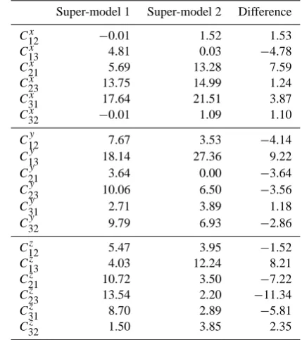
Table 2. The connection coefficients of two super-model solutions

of the Lorenz 63 system and their differences.

Super-model 1 Super-model 2 Difference

C₁₂x −0.01 1.52 1.53

C₁₃x 4.81 0.03 −4.78

C₂₁x 5.69 13.28 7.59

C₂₃x 13.75 14.99 1.24

C₃₁x 17.64 21.51 3.87

C₃₂x −0.01 1.09 1.10

C₁₂y 7.67 3.53 −4.14

C₁₃y 18.14 27.36 9.22

C₂₁y 3.64 0.00 −3.64

C₂₃y 10.06 6.50 −3.56

C₃₁y 2.71 3.89 1.18

C₃₂y 9.79 6.93 −2.86

C₁₂z 5.47 3.95 −1.52

C₁₃z 4.03 12.24 8.21

C₂₁z 10.72 3.50 −7.22

C₂₃z 13.54 2.20 −11.34

C₃₁z 8.70 2.89 −5.81

C₃₂z 1.50 3.85 2.35

3.2 Local minima

In the previous section we noted that there is a large fam-ily of super-model solutions with similar values of the cost function connected to the minimum found by the minimisa-tion. The minimisation was repeated starting from random values for the connection coefficients between [0, 10] that were drawn from a uniform probability distribution. In this way we found other minima that are distinct in many more connection coefficients. For one of these minima, the con-nection coefficients are shown in Table 2, together with the values for the first minimum. In the fourth column the differ-ence between the connection coefficients of minima 1 and 2 indicates that the minima are clearly distinct and do not be-long to the same family of solutions.

A plot of the attractor of the second super-model solu-tion in its phase space (not shown) looks almost exactly the same as the plots of the first super-model solution in Figs. 3 and 4. The value of the cost function for the second solution is slightly lower (0.003 instead of 0.02) and is a first indi-cation that the second solution might be better. In the next section we will use various measures to evaluate the quality of these two super-model solutions.

3.3 Quality measures

The cost function is a measure of the quality of the short term behaviour of the super-model in which the initial conditions play a role as is the case in weather predictions. To evaluate

(6)

166 L. A. Van den Berge et al.: Combining imperfect models through learning

Van den Berge et al.: Combining imperfect models through learning 5

x y

0 10 20 30 40 50 60

z

Truth Model 1

-20 -15 -10 -5 0 5 10 15

20 -30-20-10 0 10 20 30 z

(a) Model 1

x y

0 10 20 30 40 50 60

z

Truth Model 2

-20 -15 -10 -5 0 5 10 15

20 -30-20-10 0 10 20 30 z

(b) Model 2

x y

0 10 20 30 40 50 60

z

Truth Model 3

-20 -15 -10 -5 0 5 10 15

20 -30-20-10 0 10 20 30 z

(c) Model 3

Fig. 4. Trajectories for the three connected imperfect models with connections determined by the learning process (black) and the standard Lorenz 63 system (grey).

3.2 Local minima

In the previous section we noted that there is a large fam-ily of super-model solutions with similar values of the cost function connected to the minimum found by the minimiza-tionncd c. The minimization was repeated starting from ran-dom values for the connection coefficients between[0,10]

that were drawn from a uniform probability distribution. In this way we found other minima that are distinct in many more connection coefficients. For one of these minima, the connection coefficients are shown in table 2, together with the values for the first minimum. In the fourth column the difference between the connection coefficients of minima 1 and 2 indicates that the minima are clearly distinct and do not belong to the same family of solutions.

A plot of the attractor of the second super-model solution in its phase space (not shown) looks almost exactly the same as the plots of the first super-model solution in figures 3 and 4. The value of the cost function for the second solution is

0 0.05 0.1 0.15 0.2

7 8 9 10 11 12 13

Cy₂₃

K=20 K=50 K=100 K=150 K=200

(a)

0 0.01 0.02 0.03 0.04 0.05

8 9 10 11 12 13 14

Cz₂₁

K=20 K=50 K=100 K=150 K=200

(b)

Fig. 5. Cross section of the cost function for the super-model of the Lorenz 63 system calculated for different subsets of the original training set that was based onK= 200initializations. The subsets vary in the number of initializations, i.e. K= 20,50,100,150. A cross sections is created by changing connection coefficientsC₂₃y in (a) andC21z in (b) and keeping the other coefficients fixed at the

val-ues of the minimum found by the learning process using the training set.

Van den Berge et al.: Combining imperfect models through learning 5

x y

0 10 20 30 40 50 60

z

Truth Model 1

-20 -15 -10 -5 0 5 10 15

20 -30-20-10 0 10 20 30 z

(a) Model 1

x y

0 10 20 30 40 50 60

z

Truth Model 2

-20 -15 -10 -5 0 5 10 15

20 -30-20-10 0 10 20 30 z

(b) Model 2

x y

0 10 20 30 40 50 60

z

Truth Model 3

-20 -15 -10 -5 0 5 10 15

20 -30-20-10 0 10 20 30 z

(c) Model 3

Fig. 4. Trajectories for the three connected imperfect models with connections determined by the learning process (black) and the standard Lorenz 63 system (grey).

3.2 Local minima

In the previous section we noted that there is a large fam-ily of super-model solutions with similar values of the cost function connected to the minimum found by the minimiza-tionncd c. The minimization was repeated starting from ran-dom values for the connection coefficients between [0,10]

that were drawn from a uniform probability distribution. In this way we found other minima that are distinct in many more connection coefficients. For one of these minima, the connection coefficients are shown in table 2, together with the values for the first minimum. In the fourth column the difference between the connection coefficients of minima 1 and 2 indicates that the minima are clearly distinct and do not belong to the same family of solutions.

A plot of the attractor of the second super-model solution in its phase space (not shown) looks almost exactly the same as the plots of the first super-model solution in figures 3 and 4. The value of the cost function for the second solution is

0 0.05 0.1 0.15 0.2

7 8 9 10 11 12 13

Cy₂₃

K=20 K=50 K=100 K=150 K=200

(a)

0 0.01 0.02 0.03 0.04 0.05

8 9 10 11 12 13 14

Cz₂₁

K=20 K=50 K=100 K=150 K=200

(b)

Fig. 5. Cross section of the cost function for the super-model of the Lorenz 63 system calculated for different subsets of the original training set that was based onK= 200initializations. The subsets vary in the number of initializations, i.e. K= 20,50,100,150. A cross sections is created by changing connection coefficientsC₂₃y in (a) andC21z in (b) and keeping the other coefficients fixed at the

val-ues of the minimum found by the learning process using the training set.

Fig. 5. Cross section of the cost function for the super-model of the Lorenz 63 system calculated for different subsets of the original training

set that was based onK= 200 initializations. The subsets vary in the number of initializations, i.e.K= 20, 50, 100, 150. A cross sections is created by changing connection coefficientsC₂₃y in (a) andC₂₁z in (b) and keeping the other coefficients fixed at the values of the minimum found by the learning process using the training set.

Table 3. Mean, standard deviation (SD) and covariance for the three

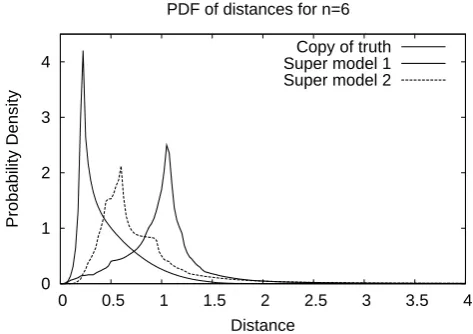
unconnected imperfect models of the Lorenz 63 system. The values for the first two models are calculated analytically. Statistics for model 3 are based on 500 runs of 5000 time units. Between brackets the 95 % error estimation is given.

Model 1 Model 2 Model 3

Meanx ±7.94 ±7.93 0.003 (0.002) Meany ±7.94 ±7.93 0.003 (0.010) Meanz 18.00 17.00 34.23 (0.030)

SDx 0 0 7.628 (0.002)

SDy 0 0 9.416 (0.010)

SDz 0 0 8.765 (0.030)

Cov. xy 0 0 58.19 (0.036)

Cov. xz 0 0 0.007 (0.44)

Cov. yz 0 0 0.012 (0.68)

the quality of the super-model beyond the range that is in-fluenced by the initial conditions, different measures can be used as in climate simulations.

The most straightforward measures are the different mo-ments of the probability density function of the states in phase space, such as the mean, variance and covariance of the state variables. Since these do not take into account the temporal evolution through phase space, we will also evalu-ate the ability of the super-model to reproduce the autocorre-lation functions of the state variables. As a final measure we will check the ability of the super-model to synchronize with the truth at the end of this section.

Table 4. Mean, standard deviation (SD) and covariance for the truth

and for the two super-models of the Lorenz 63 system. Statistics are based on 500 runs of 5000 time units. Between brackets the 95 % error estimation is given.

Truth Super-model 1 Super-model 2

Meanx −0.006 (0.22) 0.007 (0.21) −0.000 (0.25) Meany −0.006 (0.22) 0.007 (0.21) −0.000 (0.25) Meanz 23.549 (0.02) 22.93 (0.02) 23.19 (0.03)

SDx 7.924 (0.005) 7.717 (0.003) 7.812 (0.005) SDy 9.011 (0.008) 8.791 (0.009) 8.723 (0.009) SDz 8.623 (0.025) 8.596 (0.016) 8.549 (0.032)

Cov. xy 62.786 (0.07) 58.952 (0.05) 60.6416 (0.08) Cov. xz −0.020 (0.76) 0.023 (0.74) 0.000 (0.88) Cov. yz −0.016 (0.61) 0.021 (0.65) −0.001 (0.69)

Mean, standard deviation and covariance

The calculation of these statistics is based on 500 runs of 5000 time units of the truth, the imperfect models and both super-models. An error estimation of these quantities is based on the spread of the 500 estimates of each quantity. The results for the imperfect models are given in Table 3 and for the truth and both super-models in Table 4.

For the parameter values of model 1 and 2 the attractor reduces to two stable point attractors. Thex,y andz val-ues of these fixed points can be calculated analytically from Eqs. (1) by setting the time derivatives to zero. Since the sys-tem settles in one of these point attractors depending on the initial condition, the mean values are equal to these values.

(7)

L. A. Van den Berge et al.: Combining imperfect models through learning 167

6 Van den Berge et al.: Combining imperfect models through learning

0 0.05 0.1 0.15 0.2

7 8 9 10 11 12 13

Cy₂₃

(a)

0 0.01 0.02 0.03 0.04 0.05

8 9 10 11 12 13 14

Cz₂₁

(b)

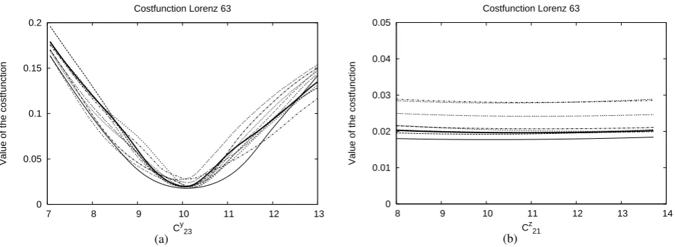
Fig. 6. As in figure 5, except that the cost function is calculated for the training set withK= 200initializations (thick line) and 9 additional independent sets of observations of the same length (thin lines) that were taken from a consecutive longer integration of the truth.

slightly lower (0.003 instead of 0.02) and is a first indication that the second solution might be better. In the next section we will use various measures to evaluate the quality of these two super-model solutions.

3.3 Quality measures

The cost function is a measure of the quality of the short term behaviour of the super-model in which the initial conditions play a role as is the case in weather predictions. To evaluate the quality of the super-model beyond the range that is in-fluenced by the initial conditions, different measures can be used as in climate simulations.

The most straightforward measures are the different mo-ments of the probability density function of the states in phase space, such as the mean, variance and covariance of

C12x -0.01 1.52 1.53

Cx

13 4.81 0.03 -4.78

C21x 5.69 13.28 7.59

C23x 13.75 14.99 1.24

Cx

31 17.64 21.51 3.87

C32x -0.01 1.09 1.10

C₁₂y 7.67 3.53 -4.14

C13y 18.14 27.36 9.22

C₂₁y 3.64 0.00 -3.64

C₂₃y 10.06 6.50 -3.56

C31y 2.71 3.89 1.18

C₃₂y 9.79 6.93 -2.86

Cz

12 5.47 3.95 -1.52

C13z 4.03 12.24 8.21

C21z 10.72 3.50 -7.22

Cz

23 13.54 2.20 -11.34

C31z 8.70 2.89 -5.81

Cz

32 1.50 3.85 2.35

Table 2.The connection coefficients of two super-model solutions of the Lorenz 63 system and their differences.

the state variables. Since these do not take into account the temporal evolution through phase space, we will also evalu-ate the ability of the super-model to reproduce the autocorre-lation functions of the state variables. As a final measure we will check the ability of the super-model to synchronize with the truth at the end of this section.

3.3.1 Mean, standard deviation and covariance

The calculation of these statistics is based on 500 runs of 5.000 time units of the truth, the imperfect models and both super-models. An error estimation of these quantities is based on the spread of the 500 estimates of each quantity. The results for the imperfect models are given in table 3 and for the truth and both super-models in table 4.

For the parameter values of model 1 and 2 the attractor reduces to two stable point attractors. Thex, y andz val-ues of these fixed points can be calculated analytically from equation (1) by setting the time derivatives to zero. Since the system settles in one of these point attractors depending on the initial condition, the mean values are equal to these values. The statistics of the chaotic solution of model 3 (see table 3) differ substantially from the truth (see table 4), espe-cially the mean value ofzis much larger.

Both super-models (see table 4) have statistics that are close to that of the truth with the largest differences of order 5% in the covariance betweenxandy. The second super-model is somewhat closer to the truth, especially in the co-variance ofxandy.

3.4 Autocorrelation

The autocorrelation is a statistical measure of the temporal evolution. It gives an indication of the memory and time

6 Van den Berge et al.: Combining imperfect models through learning

0 0.05 0.1 0.15 0.2

7 8 9 10 11 12 13

Cy₂₃

(a)

0 0.01 0.02 0.03 0.04 0.05

8 9 10 11 12 13 14

Cz₂₁

(b)

Fig. 6. As in figure 5, except that the cost function is calculated for the training set withK= 200initializations (thick line) and 9 additional independent sets of observations of the same length (thin lines) that were taken from a consecutive longer integration of the truth.

slightly lower (0.003 instead of 0.02) and is a first indication that the second solution might be better. In the next section we will use various measures to evaluate the quality of these two super-model solutions.

3.3 Quality measures

The cost function is a measure of the quality of the short term behaviour of the super-model in which the initial conditions play a role as is the case in weather predictions. To evaluate the quality of the super-model beyond the range that is in-fluenced by the initial conditions, different measures can be used as in climate simulations.

The most straightforward measures are the different mo-ments of the probability density function of the states in phase space, such as the mean, variance and covariance of

C12x -0.01 1.52 1.53

C13x 4.81 0.03 -4.78

C21x 5.69 13.28 7.59

C23x 13.75 14.99 1.24

Cx

31 17.64 21.51 3.87

C32x -0.01 1.09 1.10

C₁₂y 7.67 3.53 -4.14

C13y 18.14 27.36 9.22

C₂₁y 3.64 0.00 -3.64

C23y 10.06 6.50 -3.56

C₃₁y 2.71 3.89 1.18