Clim. Past, 9, 1089–1110, 2013 www.clim-past.net/9/1089/2013/ doi:10.5194/cp-9-1089-2013
© Author(s) 2013. CC Attribution 3.0 License.
EGU Journal Logos (RGB)
Advances in
Geosciences
Open Access
Natural Hazards
and Earth System
Sciences
Open Access
Annales
Geophysicae
Open Access
Nonlinear Processes
in Geophysics
Open Access
Atmospheric
Chemistry
and Physics
Open Access
Atmospheric
Chemistry
and Physics
Open Access
Discussions
Atmospheric
Measurement
Techniques
Open Access
Atmospheric
Measurement
Techniques
Open Access
Discussions
Biogeosciences
Open Access Open Access
Biogeosciences
Discussions
Climate
of the Past
Open Access Open Access
Climate
of the Past
Discussions
Earth System
Dynamics
Open Access Open Access
Earth System
Dynamics
Discussions
Geoscientific
Instrumentation
Methods and
Data Systems
Open Access
Geoscientific
Instrumentation
Methods and
Data Systems
Open Access
Discussions
Geoscientific
Model Development
Open Access Open Access
Geoscientific
Model Development
Discussions
Hydrology and
Earth System
Sciences
Open Access
Hydrology and
Earth System
Sciences
Open Access
Discussions
Ocean Science
Open Access Open Access
Ocean Science
DiscussionsSolid Earth
Open Access Open Access
Solid Earth
DiscussionsThe Cryosphere
Open Access Open Access
The Cryosphere
Discussions
Natural Hazards
and Earth System
Sciences
Open Access
Discussions
Climate of the last millennium: ensemble consistency of simulations
and reconstructions
O. Bothe1,2,*, J. H. Jungclaus1, D. Zanchettin1, and E. Zorita3,4
1Max Planck Institute for Meteorology, Bundesstr. 53, 20146 Hamburg, Germany 2University of Hamburg, KlimaCampus Hamburg, Hamburg, Germany
3Institute for Coastal Research, Helmholtz Centre Geesthacht, Geesthacht, Germany 4Bert Bolin Centre for Climate Research, University of Stockholm, Stockholm, Sweden
*now at: Leibniz Institute for Atmospheric Physics at the University of Rostock, K¨uhlungsborn, Germany
Correspondence to: O. Bothe ([email protected])
Received: 31 May 2012 – Published in Clim. Past Discuss.: 22 June 2012 Revised: 28 February 2013 – Accepted: 16 April 2013 – Published: 16 May 2013
Abstract. Are simulations and reconstructions of past
cli-mate and its variability consistent with each other? We assess the consistency of simulations and reconstructions for the cli-mate of the last millennium under the paradigm of a statisti-cally indistinguishable ensemble. In this type of analysis, the null hypothesis is that reconstructions and simulations are statistically indistinguishable and, therefore, are exchange-able with each other. Ensemble consistency is assessed for Northern Hemisphere mean temperature, Central European mean temperature and for global temperature fields. Recon-structions available for these regions serve as verification data for a set of simulations of the climate of the last millen-nium performed at the Max Planck Institute for Meteorology. Consistency is generally limited to some sub-domains and some sub-periods. Only the ensemble simulated and recon-structed annual Central European mean temperatures for the second half of the last millennium demonstrates unambigu-ous consistency. Furthermore, we cannot exclude consis-tency of an ensemble of reconstructions of Northern Hemi-sphere temperature with the simulation ensemble mean.
If we treat simulations and reconstructions as equitable hy-potheses about past climate variability, the found general lack of their consistency weakens our confidence in inferences about past climate evolutions on the considered spatial and temporal scales. That is, our available estimates of past cli-mate evolutions are on an equal footing but, as shown here, inconsistent with each other.
1 Introduction
Inferences about the spatiotemporal climate variability in periods without instrumental coverage rely on two tools: (i) reconstructions from biogeochemical and cultural (e.g. documentary) data that approximate the climate during the time of interest at a certain location in terms of a pseudo-observation; (ii) simulators (i.e. models) of varying complex-ity that produce discretely resolved spatiotemporal climate variables considered to represent a climate aggregation over regional spatial scales.
Thus we have no direct observational knowledge on the pre-industrial climate. Confidence in the inference on a past climate state requires reconciling models and reconstruc-tions. As a first step towards this goal, we may apply methods from numerical weather forecast verification (see, e.g. Toth et al., 2003; Marzban et al., 2011; Persson, 2011) to eval-uate the consistency of an ensemble of estimates with rele-vant verification data. These methods are less subjective than by-eye evaluations. Practically, we select a verification data target from the available reconstructions to verify an avail-able ensemble of simulations, and vice versa. For a specific task at hand, the analysis identifies whether the ensemble and the verification target are consistent realisations of the un-known past climatology or of the unun-known past climate evo-lution. We consider ensemble consistency as used in the field of weather-forecast verification (e.g. Marzban et al., 2011). Such consistency has to consider probabilistic and climato-logical properties (see below for a more detailed explanation of these two terms in the current context). Reconstructions and simulations are therefore treated as different but equi-table hypotheses, and their consistency is assessed within the framework of a statistically indistinguishable ensemble (Toth et al., 2003). The concept of indistinguishability or ex-changeability bases on the assumption that the true climate system or the target system is sampled from a distribution of model systems (compare, e.g. Toth et al., 2003; Annan and Hargreaves, 2010; Sanderson and Knutti, 2012). The target and the ensemble are indistinguishable with respect to their statistics if they are sampled from the same (or at least simi-lar) distributions. Note, to be consistent does not imply to be identical (see for example Annan et al., 2011).
The following analysis is similar to the ensemble fore-cast verification in numerical weather prediction (Toth et al., 2003) and extends the application of the paradigm of statisti-cal indistinguishability in the climate modelling context. An-nan and Hargreaves (2010) and Hargreaves et al. (2011) dis-cuss, respectively, the consistency of the CMIP3 ensemble and the ensemble consistency of the PMIP1/2 (Joussaume and Taylor, 2000; Braconnot et al., 2007) simulations in terms of this probabilistic interpretation. We adopt the Annan and Hargreaves (2010) approach to assess the mutual consis-tency among ensembles of reconstructed and simulated esti-mates of Northern Hemisphere mean temperature for the last millennium. Relevant ensembles are available for reconstruc-tions (Frank et al., 2010) and for the PMIP3-compliant Com-munity Simulations of the last millennium (COSMOS-Mill, Jungclaus et al., 2010). We further evaluate the consistency of the temporal evolutions over the last millennium of the COSMOS-Mill simulation ensemble with reconstructions for Central European mean temperature (Dobrovoln´y et al., 2010) and a temperature field reconstruction (Mann et al., 2009). Probabilistic reconstruction-simulation consistency is assessed using rank histograms (e.g. Anderson, 1996) and the decomposition of the χ2 goodness-of-fit test statistic (Jolliffe and Primo, 2008). The climatological component
of ensemble consistency is evaluated by presenting residual quantile-quantile plots (Marzban et al., 2011; Wilks, 2011). The methods are discussed in Sect. 2. Section 3 presents re-sults concerning the consistency of reconstructions and simu-lations. Appendix B discusses the robustness of the approach.
2 Methods and data
This study details case studies for the validation of ensembles of paleoclimate estimates from simulations and reconstruc-tions. We assess whether the ensembles of interest can be considered to be consistent with a relevant verification data target. We detail herein criteria for rejecting such consistency and evaluate the ensembles with respect to these criteria. This section introduces the methods and the criteria.
An ensemble of (climate) estimates can be validated against a suitable verification data target either by consider-ing individually the accuracy of each ensemble member or by evaluating the consistency of the full ensemble (e.g. Marzban et al., 2011). The latter approach may follow the methods applied in the verification of numerical weather forecast en-sembles. These are based on the concept of statistical indis-tinguishability of the ensemble, which is interpreted prob-abilistically. We assume that the verification target and the simulations are samples from a larger distribution (compare, e.g. Toth et al., 2003; Annan and Hargreaves, 2010; Persson, 2011; Sanderson and Knutti, 2012) so that their statistics are exchangeable.
Practically, exchangeability – or, analogously, indistin-guishability – refers to the assumption that the verification data may be exchanged for any member of the ensemble without changing the characteristics of the ensemble. For a consistent ensemble, the verification target and ensemble es-timated (e.g. forecasted) frequencies agree (Murphy, 1973). Thus an ensemble is probabilistically consistent if we can-not reject the hypothesis that the frequencies agree. In fore-cast ensemble verifications, an ensemble is called reliable, if we cannot reject this hypothesis according to appropri-ate tests. Since we deal with highly uncertain data, we do not use the term “reliability” here but only refer to consis-tency. The assessment of ensemble consistency provides a necessary condition for our evaluation of ensemble accuracy in paleoclimate-studies (following Annan and Hargreaves, 2010) under large uncertainties and due to the lack of an ob-served target.
2.1 Methods
2.1.1 Evaluation of probabilistic consistency
Probabilistic consistency is commonly evaluated by rank-ing the verification target data against the ensemble data (Anderson, 1996; Jolliffe and Primo, 2008; Annan and Hargreaves, 2010; Marzban et al., 2011; Hargreaves et al., 2011). Target data and ensemble data are sorted by value and the calculated ranks counted and plotted as a rank histogram (Anderson, 1996). If we expect equiprobable outcomes for an ideal, indistinguishable ensemble, the ranking should re-sult in a uniform, flat histogram.
We can test the goodness-of-fit of a rank histogram relative to the flat expectation, i.e. with respect to the null hypothe-sis of a uniform outcome. An ensemble is probabilistically consistent if we fail to reject the hypothesis of a uniform histogram. One suitable test is theχ2test (e.g. Jolliffe and Primo, 2008). Jolliffe and Primo (2008) detail how we can decompose the test statistic enabling tests for individual devi-ations from flatness which are due to different statistics of the distributions. Please see Jolliffe and Primo (2008) for a com-prehensive delineation. Appendix A presents more details on the test and discusses the chosen approach.
Besides the possibility to test for deviations from a uni-form outcome, the rank histograms already visually assist in identifying discrepancies between the ensemble data and the verification data. An apparent dome-shaped histogram in-dicates that the ensemble data is sampling from a distribu-tion which is wider than the verificadistribu-tion data distribudistribu-tion. A u-shape signals an ensemble distribution which is nar-rower than the verification data distribution. The spread of the ensemble is, respectively, overly wide or overly narrow. That is, the ensemble data differs in its variance from the verification data. We refer to too wide distributions as be-ing over-dispersive and to too narrow distributions as under-dispersive. If the ensemble is biased to large values, the rank counts display a negative trend. If it is biased to low values, the trend is positive in the rank counts. Consequently, if the ensemble data has a negative bias, the verification data will cluster in the high classes of the histogram and vice versa. Jolliffe and Primo (2008) give details on other possible de-viations, but we focus here only on biases and differences in the spread of the ensemble data.
In summary, rank histograms are a tool to disclose whether a probabilistically interpreted ensemble and its verification data represent different climates. They provide a means for evaluating the consistency of the joint distribution for the en-semble and verification data (see Wilks, 2011).
The ranking further allows mapping the ranks of the ver-ification data and thereby helps in validating gridded spa-tial data. That is, the position of the verification data within the ensemble can be visualized in maps (see Sects. 3.2.1 and 3.2.2). The rank of the verification data is plotted at each grid-point for individual time steps or for climatological
averages. Local low rank counts of the target indicate that the ensemble is biased high at the grid-point, and high ranks im-ply a low bias.
2.1.2 Evaluation of climatological consistency
Following Marzban et al. (2011, see also Wilks, 2011), we use residual quantile-quantile plots (r-q-q plots) to study the climatological consistency of the distributions for the ensem-ble with the target. Common quantile-quantile plots assess the quantiles of a distribution against a reference. For ex-ample, the quantile estimates of a hindcast simulation are plotted on the y-axis against the observed quantiles on the x-axis. Residual quantile-quantile plots only differ from this common approach by plotting the differences between the simulated distribution quantiles and the chosen verification data quantiles on the y-axis. Thereby they emphasise the de-viations between the simulated and the verification quantile distributions.
This visualisation allows assessing whether the climato-logical distribution of an estimate of interest is similar to the distribution of the target. Thus we are able to identify whether the empirical quantiles for each individual ensem-ble member agree with the verification data sample. Plotting the residuals eases the interpretation since ideal agreement between estimated and verification quantiles leads to vanish-ing residuals, i.e. a horizontal line crossvanish-ing the y-axis at zero. Thus disagreements are also easily identified. Differences in the tails of the distributions, their skewness or their means are of particular interest among the possible deviations.
Biases of the estimated distributions lead to horizontal dis-placements from the expectation of vanishing residual quan-tiles in the residual quantile-quantile plot since the mean of the estimated distribution differs from the verification refer-ence. The residuals show a positive slope if the estimated climatological distribution is wider than the verification cli-matology distribution, and a negative slope if it is narrower (Marzban et al., 2011). This reflects differences in estimated and target climatological variances. Thus if the climatologi-cal variance of the estimate is larger than that of the target, the ensemble systematically overestimates the distance be-tween the mean and the quantile locations. This results in a positive slope in the residual quantile. Smaller climatologi-cal variance results in a negative slope since the quantiles are closer to the mean. Marzban et al. (2011) give more details on the interpretation of the pattern of residual quantiles. We refer to differences in the width as over- and under-dispersion for too wide and too narrow distributions, respectively.
of the climatologies of individual simulations with the veri-fication data.
2.2 Data
We apply the described methods to the following data sets. The simulations are the COSMOS-Mill model data for the last millennium performed with the Max Planck Institute Earth System Model (ESM). This version of MPI-ESM is based on the atmosphere model ECHAM5, the ocean model MPI-OM, a land-surface module including vegetation (JSBACH), a module for ocean biogeochemistry (HAMOCC) and an interactive carbon cycle. Details of the simulations have been published by Jungclaus et al. (2010).
The set specifically includes single forcing simulations for volcanic, strong solar and weak solar forcing. Furthermore, there are five full-forcing simulations with weak solar ing and three full-forcing simulations with strong solar forc-ing. The full ensemble has eleven members. We assume that our estimates of the forcing series are highly uncertain and that this uncertainty propagates to our knowledge of their in-fluence on the pre-industrial climate. Therefore, we include the single forcing simulations as valid hypotheses about the pre-industrial climate trajectory. We denote the full ensem-ble by SIM. WSIM and SSIM refer to the full-forcing simu-lations with weak and strong solar forcing, respectively (i.e. the weak and strong ensembles). Additionally, we take ad-vantage of the 3100 yr control run describing an unperturbed climate.
The reconstructions are all for annual mean temperature. We use the regional mean time series for Central Europe by Dobrovoln´y et al. (2010), the ensemble of Northern Hemi-sphere means by Frank et al. (2010) and the global field re-construction by Mann et al. (2009). All series have an annual resolution, but some are temporally smoothed (e.g. Mann et al., 2009).
The Frank et al. (2010) data is the only available ensemble of reconstructions. Frank et al. (2010) recalibrate a number of previous reconstructions to various periods of instrumen-tal observations, thereby obtaining an ensemble of 521 recal-ibrated reconstruction series (see Frank et al., 2010, for dis-cussions on the ensemble construction). The ensemble bases on the reconstructions by Jones et al. (1998), Briffa (2000), Mann and Jones (2003), Moberg et al. (2005), D’Arrigo et al. (2006), Hegerl et al. (2007), Frank et al. (2007), Juckes et al. (2007) and Mann et al. (2008). The original reconstructions end at different dates, that is, their last available annual data differ. We refer to the full 521 member ensemble as FRA. The choice of the calibration window strongly influences the variability of the reconstructions which is going to influence subsequent analyses. The 1920–1960 period likely presents the most reliable observational data if we want to use all nine reconstructions. Therefore, in the following, we use the sub-ensemble re-calibrated to the period 1920 to 1960 and refer to it as FRS.
We interpolate the spatial field data on a 5◦×5◦grid. Our
general interest is in the consistency of paleoclimate recon-structions and simulations for the last millennium. There-fore we take anomalies with respect to the common period of reconstructions and simulations but exclude the period of overlap with the modern observations. European anomalies are for the period 1500 to 1854 relative to the mean from 1500 to 1849. For the Northern Hemisphere data, we com-pute anomalies for the period 1000 to 1849 and relative to the mean for the same period. The decadally smoothed global fields for the years 805 to 1845 are centred relative to the mean for the period 800 to 1849. We further consider four sub-periods in the analyses of the global field data. These consist of 250 non-overlapping records from the full pe-riod 805 to 1845. The first three pepe-riods cover the first 750 records, and the last period covers the last 250 records.
The rank histogram approach (see Sect. 2.1) assumes that the validation data sets include errors (Anderson, 1996) that have to be included in the ensemble data. If the reconstruc-tions are reported with an uncertainty estimate, this is used to inflate the simulated data.
For the Central European data, the uncertainty is sampled from a normal distribution with zero mean and standard de-viation equal to the one standard error estimate given by Do-brovoln´y et al. (2010). No uncertainty estimate is given for the global field data. However, Mann et al. (2009) provide standard errors for their unscreened Northern Hemisphere mean temperature series. We assume that the largest standard error reported for this data is a reasonable guess for an un-certainty estimate for the field data as well. Thus we choose to inflate the ensemble at each grid-point by a random uncer-tainty estimate drawn from a Gaussian distribution with stan-dard deviation equal to this stanstan-dard error (i.e.σ=0.1729). The SIM and the FRS data are ensembles. Thus we can randomly sample an “observational” uncertainty for their en-semble means from a distribution with zero mean and stan-dard deviation equal to the ensemble stanstan-dard deviation at each point. For the analyses relative to an ensemble mean, we additionally use additive internal variability estimates for the target data (see Sect. 2.3 for details).
As mentioned above, the way we construct the FRS en-semble influences the enen-semble spread and thus the results. We account for this sensitivity by basing the uncertainties for the ensemble-mean reconstruction on the full FRA-ensemble spread.
2.3 Discussion of the chosen approach
et al. (2011) further discuss the influence of intra-ensemble correlations and correlations between the ensemble and the verification target on the rank histogram.
One of the most important limitations of the rank his-togram approach is that uniformity in rank hishis-tograms may result from opposite biases or opposite deviations in spread in different periods which may cancel out (Hamill, 2001). Fur-thermore, temporal correlations in the data can result in pre-mature rejection of consistency (Marzban et al., 2011). We use bootstrapped estimates and analyse different sub-periods at individual grid points to address these problems.
Rank histograms may be misleading since they are af-fected by the amount of correlations between verification and ensemble or within the ensemble and the differences between both (Marzban et al., 2011). We assume that these caveats increase the general uncertainty in the comparison between simulations and reconstructions of past climate states and variability.
We may evaluate the consistency of simulations and re-constructions on three levels of resolution: area-averaged time series, gridded spatio(-temporal) data, or individual grid points of gridded data sets. Obviously, results may differ be-tween these levels. Further, it is not easy to know a priori whether we should expect larger consistency at one of the resolutions. Note that even if we find an ensemble of sim-ulations to be consistent at the grid-point level, we cannot say whether the covariance between individual grid points is consistent with the covariability in the verification data.
We assume that the data sets represent inter-annual varia-tions of a temperature index. This is not necessarily valid. If the target is an ensemble mean, it displays reduced variability compared to the ensemble members especially on the inter-annual time scale. Thus using an ensemble mean as verifica-tion target impacts the ensemble consistency. We argue that the inherent uncertainty of the target may compensate for this reduced variability caused by ensemble averaging. Assum-ing that reconstruction and simulation ensemble estimates in-clude the same externally forced variability, the target ensem-ble mean should essentially recover the forced signal within the propagated uncertainties. Furthermore, the probabilistic ensemble estimates should reliably represent the target dis-tribution if the ensemble includes the target uncertainty.
Nonetheless, in the following we pursue an alternative approach to compensate for the reduced variability of an ensemble-mean target and add an estimate of the inter-nal variability to the ensemble-mean estimate. In assessing the consistency of the SIM ensemble, we first compute the residual deviations of the full FRA-reconstruction ensemble from its ensemble mean. Then, we fit autoregressive-moving-average models to the residuals. Thereby we obtain 521 pos-sible fits. We produce 10 random representations of the pro-cess for each fit. If we add these 5210 estimates of residual internal variability to the ensemble mean, we obtain a set of targets. For the assessment of the FRS ensemble, we add one section of the MPI-ESM control run (Jungclaus et al., 2010)
to the SIM-ensemble mean. Since we further account for the sampling variability, using one segment is robust enough for evaluating the unforced internal variability of the simula-tions.
Finally, FRA- and FRS-ensemble members are to some extent time-filtered. They exhibit by construction reduced variability on inter-annual time-scales (compare, e.g. Franke et al., 2013). As the filter-properties differ, we do not account for this filtering. On the other hand, we use decadal mov-ing means for the SIM data to compensate for the decadal smoothing of the global field data (Mann et al., 2009).
Appendix B supplements our assessment of mutual simulation-reconstruction consistency by presenting eval-uations of the self-consistency for both the control run and the FRS ensemble. The first allows assessing the self-consistency of the unperturbed simulated climate and the sensitivity of our tests. The second allows evaluating the large uncertainty in our reconstructed estimates and of the available targets for evaluating the simulations.
3 Results
We first evaluate the consistency of the SIM ensemble rela-tive to two reconstruction targets: the Central European tem-perature data by Dobrovoln´y et al. (2010) and the ensem-ble mean of the Northern Hemisphere temperature FRA en-semble. In a reverse analysis, we then test whether the FRS ensemble is consistent with the ensemble mean of the SIM-ensemble. SIM, WSIM and SSIM are further analysed for their consistency with individual members of the FRS-data. Finally, we assess the ensemble consistency of the SIM-ensemble with the global field reconstruction by Mann et al. (2009).
3.1 Area-averaged time series
Figures 1 to 3 provide a first impression of the ensemble data sets and the respective verification target series. We display the target time series and their variability together with the range of the ensembles.
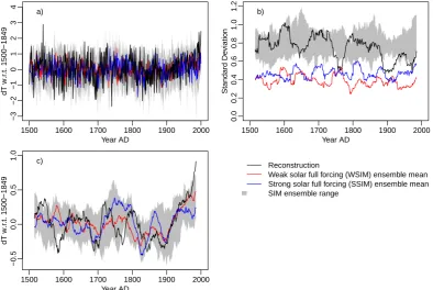
The European data for the SIM ensemble and its recon-structed verification target cover a similar range and show similar variability (Fig. 1). Note that the SSIM and WSIM ensemble means exhibit a reduced variability compared to the full ensemble range of variability (Fig. 1b).
1500 1600 1700 1800 1900 2000
−3
−2
−1
0
1
2
3
4
Year AD
dT w.r
.t. 1500−1849
a)
1500 1600 1700 1800 1900 2000
0.0
0.2
0.4
0.6
0.8
1.0
1.2
Year AD
Standard De
viation
b)
1500 1600 1700 1800 1900 2000
−0.5
0.0
0.5
1.0
Year AD
dT w.r
.t. 1500−1849
c)
Reconstruction
Weak solar full forcing (WSIM) ensemble mean Strong solar full forcing (SSIM) ensemble mean SIM ensemble range
Fig. 1. (a) Time series, (b) moving 31 yr standard deviations and (c) moving 31 yr means for the Central European annual temperature data. Black is the target data and transparent light grey shading is the range of the ensemble. Red (blue) lines are for the WSIM (SSIM) full-forcing simulation ensemble means.
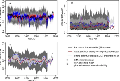
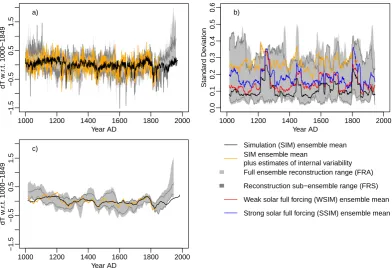
Including the estimates of internal variability increases the range of possible temporal evolutions of the reconstructed verification targets for the SIM ensemble (Fig. 2). In con-trast, the verification target for the FRS ensemble does not change too much if we include an estimate of internal vari-ability (Fig. 3). Nevertheless, we see a pronounced increase in the variability of the SIM ensemble mean. Sections 3.1.2 and 4 discuss the influence of the resolved variability on the results.
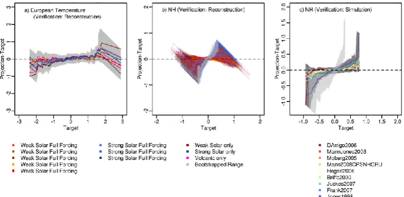
Figures 4 and 5 illustrate the analyses of, respectively, the probabilistic and the climatological consistency for these three ensemble-data sets. Both figures account for the un-certainty in the verification target as described in Sect. 2.2. Uncertainty estimates are the reported standard errors for the Central European temperature target (Dobrovoln´y et al., 2010) and the spread of the mutual ensembles for the North-ern Hemisphere data targets. If we neglect these “observa-tional” uncertainties in the verification data the conclusions change for the hemispheric data (not discussed).
3.1.1 Ensemble consistency of area-averaged estimates
The rank counts plotted in Fig. 4a indicate that we cannot reject consistency of the SIM ensemble data for the annual mean Central European temperature with the reconstruction verification target. Nevertheless, the test statistics for a devia-tion in spread are significant, implying a lack of consistency.
Interestingly, the bootstrapped rank count intervals enclose the possibility of a uniform rank count, i.e. of consistency. The contrast between bootstrap and goodness-of-fit test pos-sibly highlights the problem of sampling variability.
The results differ for the assessment of probabilistic con-sistency of the hemispheric estimates depending on whether or not we account for internal variability in the ensemble-mean target data (Fig. 4b,c). We first consider the case where the assessment does not include the estimates of internal vari-ability described in Sect. 2.3. Then, for the evaluation of the SIM ensemble, the dome-shaped histogram in Fig. 4b shows that the verification target occupies too often the central ranks, i.e. the SIM ensemble is significantly over-dispersive. The bootstrapped intervals confirm this (cyan overlay in Fig. 4b). Similarly the FRS ensemble is too wide relative to the Northern Hemisphere target of the simulation-ensemble mean if we do not account for the reduced internal variability (cyan overlay in Fig. 4c).
1000 1200 1400 1600 1800 2000
−1.5
−0.5
0.5
1.0
1.5
Year AD
dT w.r
.t. 1000−1849
a)
1000 1200 1400 1600 1800 2000
0.0
0.2
0.4
0.6
Year AD
Standard De
viation
b)
1000 1200 1400 1600 1800 2000
−0.5
0.0
0.5
1.0
Year AD
dT w.r
.t. 1500−1849
c)
Reconstruction ensemble (FRA) mean
Weak solar full forcing (WSIM) ensemble mean
Strong solar full forcing (SSIM) ensemble mean
SIM ensemble range FRA ensemble mean
plus estimates of internal variability
Fig. 2. (a) Time series, (b) moving 31 yr standard deviations and (c) moving 31 yr means for the SIM Northern Hemisphere temperature data against the reconstructed target. Black is the verification data target and transparent light grey shading is the range of the SIM ensemble. Red (blue) lines are for the WSIM (SSIM) full-forcing simulation ensemble means. Dark grey shading is the range of the reconstruction ensemble-mean target with added internal variability estimates. Here and in Fig. 3, the data including the estimate for internal variability is only shown for the period of analysis from the start of the millennium to the mid-19th century.
On the other hand, FRS is consistent with the ensemble-mean simulation target when we include the estimate of in-ternal variability for the simulation. That is, deviations from a flat histogram are negligible for the continuous black line in Fig. 4c and the test statistics are also not significant. The bootstrapped ranks (grey shading in Fig. 4c) further highlight the good probabilistic agreement under the made assump-tions. The reconstructions by Hegerl et al. (2007), Mann and Jones (2003) and Mann et al. (2008) are filtered estimates, but the conclusions do not change if we include an arbitrarily chosen estimate of internal variability in these three series.
The climatological quantiles support the probabilistic as-sessment. They agree rather well between the SIM ensem-ble members and the Central European temperature target data. The residual quantiles align more or less close to zero in Fig. 5a. Some simulations appear to underestimate very warm anomalies and overestimate very cold anomalies. A slight positive slope occurs in the residual quantiles but we conclude that this over-dispersive tendency is not significant since the bootstrapped intervals still include the zero line.
The climatological deviations between the quantiles for the Northern Hemisphere temperature in SIM and the tar-get are larger than for the Central European data. The SIM members give positively sloped residual quantiles, i.e. overly wide climatological distributions, if we do not account for
the reduced internal variability in the relevant target (the FRA ensemble mean) (grey overlay in Fig. 5b). Similarly, FRS en-semble members generally overestimate at least the positive anomaly quantiles relative to the target (the SIM ensemble mean) if we exclude the internal variability estimate (trans-parent grey in Fig. 5c).
1000 1200 1400 1600 1800 2000
−1.5
−0.5
0.5
1.5
Year AD
dT w.r
.t. 1000−1849
a)
1000 1200 1400 1600 1800 2000
0.0
0.1
0.2
0.3
0.4
0.5
0.6
Year AD
Standard De
viation
b)
1000 1200 1400 1600 1800 2000
−1.5
−0.5
0.5
1.5
Year AD
dT w.r
.t. 1000−1849
c) Simulation (SIM) ensemble mean
SIM ensemble mean
plus estimates of internal variability Full ensemble reconstruction range (FRA)
Reconstruction sub−ensemble range (FRS)
Weak solar full forcing (WSIM) ensemble mean
Strong solar full forcing (SSIM) ensemble mean
Fig. 3. (a) Time series, (b) moving 31 yr standard deviations and (c) moving 31 yr means for the FRA Northern Hemisphere temperature reconstruction ensemble against the simulated target. Black is the verification data target and transparent light grey shading is the range of the FRA ensemble. Dark grey lines mark the range of the FRS reconstruction sub-ensemble recalibrated to the period 1920–1960. The orange line is the estimate of the target with added internal variability estimate. In (b) red (blue) lines are for the weak (strong) solar full-forcing simulation ensemble means.
2 4 6 8 10 12
0
20
40
60
Rank
Counts
● ●
● ●
● ●
●
● ●
● ●
● ●
● ● ●
● ● ●
● ● ●
●
● Bias 0.04
Spread 3.17 a)
2 4 6 8 10 12
0
50
100
150
200
250
Rank
Counts
● ●
● ●
● ●
●
●
● ●
● ● ●
● ●
● ●
● ●
●
● ●
● ● Median Bias 0.13
Median Spread 55.81 b) NH (Verification: Reconstruction)
2 4 6 8 10
0
50
100
150
200
250
Rank
Counts
● ●
● ● ●
● ●
●
● ● ●
● ●
● ●
● ●
●
● ● Bias 0.05
Spread 0.25
c) NH (Verification: Model)
Fig. 5. Evaluation of climatological consistency: residual quantile-quantile plots for temperature data: (a) SIM members against Central Eu-ropean annual temperature target, (b) SIM members against Northern Hemisphere temperature target, (c) FRS against Northern Hemisphere temperature target. Panels account for the uncertainties in the target. See legend for individual ensemble members. Grey shading in (a) and transparent grey overlay in (b–c) are 0.5 % and 99.5 % quantiles for block-bootstrapped residual quantiles (2000 replicates, block length of 50 yr). In (b) we plot all results relative to all used targets including an estimate of internal variability. In (c) the dark grey shading are the bootstrapped quantiles relative to the target including an estimate of simulated internal variability. Middle grey (c) is due to the transparency.
(see above, Fig. 4b) where we also find a generally over-dispersive character of the SIM ensemble.
For the FRS ensemble, we generally find good agreement between the quantiles of the ensemble members and the sim-ulation target if we include an estimate of internal variabil-ity in the target (Fig. 5c). For most members, large residuals occur only in the tails of the distribution. The bootstrapped intervals emphasise this general consistency by including the zero line of vanishing residuals. The deviations in the tails are most pronounced for large negative anomalies in the re-construction by D’Arrigo et al. (2006). An exception to this general description is the data set by Jones et al. (1998). For this reconstruction a strong positive slope in the residuals in-dicates a strong dispersive character. Much of the over-dispersion comes from the large associated uncertainties.
The next paragraphs complement the above results by shortly looking at some sub-divisions of the considered SIM and FRS ensemble. Since the SIM ensemble encapsulates the SSIM and WSIM ensembles, we shortly discuss the con-sistency of these two sub-ensembles. We consider the un-certainty and, for the hemispheric data, also include inter-nal variability estimates. For the sake of brevity, we just re-port the results. Generally, results for the two sub-ensembles agree well with those found for the full SIM ensemble rel-ative to the Central European temperature. However, both, SSIM and WSIM, display specific behaviours. WSIM is un-ambiguously probabilistically consistent with the European reconstructions, but SSIM is slightly too wide. SSIM devia-tions in the spread are significant according to the goodness-of-fit test. However, the bootstrapped intervals suggest that
this may be due to sampling variability. Results for the cli-matological consistency are similar for SSIM and WSIM as seen in the SIM assessment in Fig. 5a.
With respect to the Northern Hemisphere mean target, the WSIM ensemble is probabilistically too wide while we are only able to make ambiguous statements for SSIM. Since the SSIM ensemble has only three members, we have any-way to be careful when interpreting the results. The single deviation test for spread suggests significant over-dispersion. However, the bootstrapped rank intervals do not allow reject-ing consistency since they safely include the possibility of a flat histogram. The residual quantiles display a wide range of possible deviations for SSIM (compare Fig. 5b).
For the reversed verification, the single deviation tests in-dicate significant spread deviations of the FRS reconstruc-tion ensemble. It is slightly too narrow if the target is the WSIM ensemble mean, but strongly too narrow if the tar-get is the SSIM ensemble mean. However, the bootstrapped intervals again allow for consistency relative to both SSIM and WSIM. Climatologically, most FRS ensemble members are consistent with both targets but again the results are dis-tinct for the reconstruction by Jones et al. (1998). That is, for all FRS members the climatological deviations relative to the SSIM and WSIM ensemble-mean targets are similar to those relative to the SIM ensemble mean (compare Fig. 5c), but the residuals are larger when evaluated against the SIM ensemble-mean target.
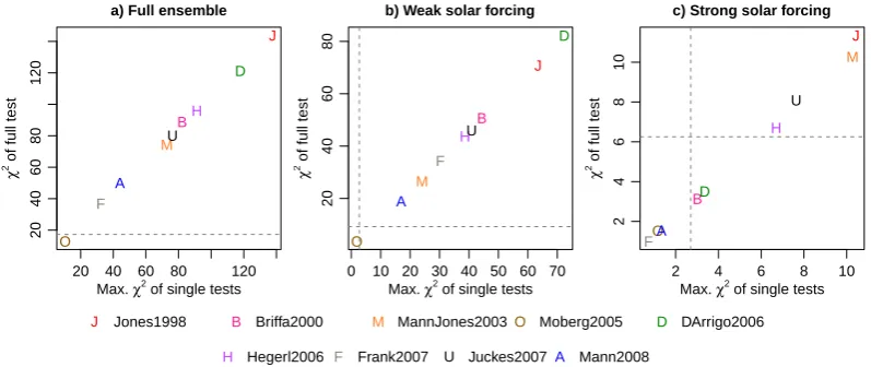
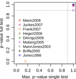
ensemble relative to individual reconstructions. We shortly present results on the assessment of SIM, SSIM and WSIM relative to the FRS ensemble members as targets. Here, we include uncertainty estimates. Furthermore, we add an arbi-trary member of the ensemble of estimates of internal vari-ability estimates (see Sect. 2.3) to the three filtered recon-structions by Hegerl et al. (2007), Mann and Jones (2003) and Mann et al. (2008). Figure 6 presents theχ2values for the tests.
Obviously, the SIM ensemble lacks probabilistic consis-tency with all reconstructions according to theχ2test (con-sidering our assumptions on internal variability and uncer-tainty). The bootstrapped intervals confirm this (not shown). The full test gives no significant results relative to the recon-struction by Moberg et al. (2005). Climatological quantiles confirm the probabilistic findings (not shown).
WSIM appears to be probabilistically consistent with the Moberg et al. (2005) reconstruction. The bootstrapped inter-vals suggest that the ensemble is not inconsistent with the data by Mann et al. (2008) under the made assumptions (not shown). Residual quantiles are large except relative to the re-construction by Moberg et al. (2005).
The three-member SSIM ensemble is a special case. Boot-strapped intervals do not allow to reject probabilistic consis-tency for any of the nine reconstructions under the assump-tions on internal variability and uncertainty. Test statistics in Fig. 6c indicate consistency of the ensemble with the data by Frank et al. (2007), Moberg et al. (2005) and Mann et al. (2008). Again, residual quantiles are large except for the re-construction by Moberg et al. (2005).
In summary, verification of the SIM ensemble suggests that it is likely too wide relative to the ensemble mean of the Northern Hemisphere mean temperature reconstructions. Discrepancies arise not only probabilistically but also in the climatologies. The climatological results may depend on the representation of the internal variability in the verification target. The FRS ensemble for Northern Hemisphere temper-ature, on the other hand, appears to be consistent with its target (the SIM ensemble mean) if we account for uncer-tainties and internal variability. Nevertheless, most ensem-ble members display climatological deviations in the tails of the distribution. In the end, the large uncertainties in the en-sembles and in the verification targets generally prohibit re-jecting consistency for the Northern Hemisphere estimates. The results are more encouraging for the considered regional temperature estimate. The SIM estimates for the Central Eu-ropean temperature appear to be unambiguously consistent with the respective target.
3.1.2 Addressing lack of consistency of area-averaged estimates
Returning to Figs. 1 to 3, the following notes are worth re-peating. First, while the SIM ensemble covers a similar range of temperature values as the Central European reconstruction
target and while their variability is also similar, the low-frequency variability differs notably between the ensemble and the target (Fig. 1b). Secondly, differences between SIM and the northern hemispheric target are prominent and also between FRS and its target (Figs. 2 and 3). Furthermore, with respect to the hemispheric data, the range of the re-constructed targets is relatively wide compared to the SIM ensemble spread if we account for the reduced internal vari-ability in the original FRA ensemble-mean target. The mov-ing standard deviations emphasise the disagreement in vari-ability (Fig. 2b). For the FRS ensemble, on the other hand, including an estimate of internal variability does not unduly change the respective target (Fig. 3a). However, the variabil-ity of the target increases notably (Fig. 3b).
Thus ensemble data can be statistically indistinguishable from a verification target although their trajectories evolve notably different over much of the considered time-span. This is seen for the Central European temperature data (Figs. 1c, 4a, 5a) in both the probabilistic and the climato-logical assessment. That is, the strong differences in the 18th century (or similarly the late 1500s) are consistent with our knowledge about internal and externally forced climate vari-ability for the continent under the uncertainties associated with reconstructions, climate simulations and the forcing re-constructions.
This obviously does not hold for the hemispheric data of the SIM ensemble for which the probabilistic and climato-logical evaluations reveal disagreements with the target. The time series in Fig. 2 clarify that part of the over-dispersive character of the hemispheric SIM data may relate to (i) biases in the periods 1000 to 1300 and 1500 to 1650, when recon-structions and simulations evolve to some extent in opposite way, and to (ii) less warming in the target in the 18th century. The same biases act in opposite directions in the evaluation of the hemispheric data of the FRS ensemble. However, here the biases are not large enough to allow rejecting consistency. Indeed, they compensate over the full period.
20 40 60 80 120
20
40
60
80
120
a) Full ensemble
Max. χ2 of single tests
χ
2 of full test
J
B
M
O
D
H
F U
A
0 10 20 30 40 50 60 70
20
40
60
80
b) Weak solar forcing
Max. χ2 of single tests
χ
2 of full test
J
B
M
O
D
H
F U
A
2 4 6 8 10
2
4
6
8
10
c) Strong solar forcing
Max. χ2 of single tests
χ
2 of full test
J
B
M
O D
H
F
U
A
J Jones1998 B Briffa2000 M MannJones2003O Moberg2005 D DArrigo2006
H Hegerl2006 F Frank2007 U Juckes2007A Mann2008
Fig. 6. Assessing SIM, WSIM and SSIM ensembles against individual reconstructions of Northern Hemisphere temperature (members of FRS ensemble). Uncertainties are considered, and internal variability estimates are included in the data by Hegerl et al. (2007), Mann and Jones (2003) and Mann et al. (2008) to account for the temporal filtering of the individual reconstructions. (a) SIM:χ2statistics for the full test against the maximum of the decomposedχ2statistics obtained for the tests for bias and spread deviations. (b) as in (a) but for the five-member WSIM ensemble. (c) as in (a) but for three-member SSIM. Vertical and horizontal grey lines mark thoseχ2statistics for which leftpvalues are larger than 0.9 for the distributional degrees of freedom.
for an ensemble-mean reconstruction as target still represent the different methodologies and the different types of proxy data although the estimates are generated as stochastic pro-cesses.
Our presented analyses deal with data sets which either have similar variability (the Central European data) or for which we have to account for reductions in internal variabil-ity since we employ ensemble-mean targets. However, strong discrepancies occur also between SIM and reconstructions which are resolved at inter-annual time-scales (not shown).
3.2 Spatial fields
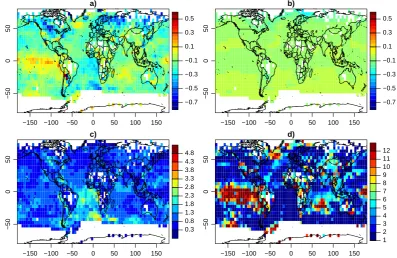
Figure 7 gives some information on the global temperature data for an arbitrarily chosen sub-period (1390s to 1690s) as they are depicted by reconstructions (Fig. 7a) and simu-lations (ensemble mean in Fig. 7b, compare also Fig. 7 of Fern´andez-Donado et al., 2013). Comparison of Fig. 7a and b highlights how strongly mean anomalies of the SIM en-semble may disagree with the target pattern for this specific period.
While the ensemble mean, of course, smoothes out the patterns found in individual runs, it is noteworthy, that not only the SIM ensemble but also a multi-model ensemble (Fern´andez-Donado et al., 2013, compare their Fig. 7) cap-ture basically none of the reconstructed feacap-tures for this pe-riod. This potentially highlights the limited value of such simple comparisons. The most prominent mismatch between the ensemble and the target is found in the tropical Pacific (compare Fig. 7a, b, d). This strong signal is less due to the strong ENSO variability in MPI-ESM (compare Jungclaus et al., 2006), but more due to the contrast between the warm
mean anomaly of the target and the diverse but generally much weaker mean anomalies in the SIM ensemble. Simula-tions incorporating a strong solar forcing even display nega-tive anomalies (not shown). Such a La Ni˜na-like response not only conflicts with the target, but also contrasts with the find-ings during solar forcing minima by Meehl et al. (2009) and Emile-Geay et al. (2007); see also the discussions by Misios and Schmidt (2012) on the relationship between solar insola-tion maxima and tropical Pacific sea surface temperatures.
In the following, we evaluate the consistency of the SIM ensemble relative to the decadally smoothed global temper-ature fields. We repeat that deviations from a uniform rank histogram count may be due to biases or differing spread in particular periods, while the ensemble is consistent with the target in other periods. Discrepancies can easily be identified when analysing single time series but assessments of consis-tency are not easily visualised at the grid-point level of spatial fields. We use different time periods to account for possible changes in deviations over time. We employ sub-periods of non-overlapping 250 records in the range from 805 to 1845. The first three periods cover the first 750 records of the full data (about 805 to 1055, 1055 to 1305, 1305 to 1555) while the last period covers the last 250 records of the data sets (about 1595 to 1845). Thus there is a gap between the earlier three periods and the late period.
−150 −100 −50 0 50 100 150
−50
0
50
a)
Longitude
Latitude[3:34]
−0.7 −0.5 −0.3 −0.1 0.1 0.3 0.5 0.7
−150 −100 −50 0 50 100 150
−50
0
50
b)
Longitude
Latitude[3:34]
−0.7 −0.5 −0.3 −0.1 0.1 0.3 0.5 0.7
−150 −100 −50 0 50 100 150
−50
0
50
c)
0.3 0.8 1.3 1.8 2.3 2.8 3.3 3.8 4.3 4.8
−150 −100 −50 0 50 100 150
−50
0
50
d)
1 2 3 4 5 6 7 8 9 10 11 12
Fig. 7. Global fields of decadally smoothed temperature: (a) reconstructed mean anomaly map for a cold period (for the 1390s to 1690s), (b) ensemble-mean simulated anomaly map for the same period, (c) ensemble mean of relative standard deviations (reconstruction standard deviation divided by simulation standard deviation at each grid-point for the full period), (d) mapped target ranks for evaluating SIM against the target for the cold period (1390s to 1690s).
to this standard error. Without uncertainty inflation, the ex-pected effective rank frequencies can be very small due to the temporal auto-correlations in the data. The number of in-dependent samples is always largest over the tropical Pacific (not shown) probably due to the too strong and too regular ENSO in MPI-ESM (Jungclaus et al., 2006).
3.2.1 Ensemble consistency of spatial fields
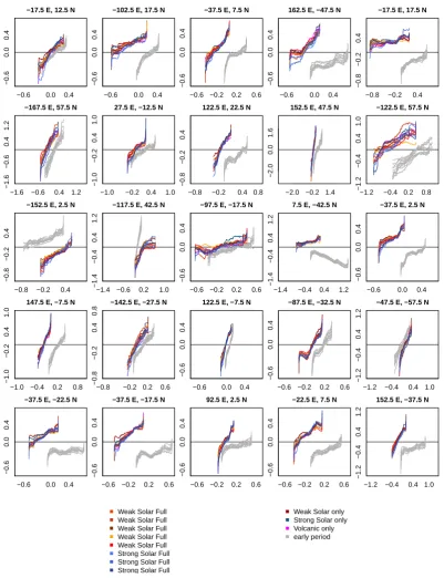
Figures 8 to 10 display a selection of results for the eval-uation of consistency of the SIM ensemble with the global temperature field reconstruction by Mann et al. (2009) at in-dividual grid points. As for the time series data, the most common deviation is a too wide ensemble. This holds for the probabilistic assessment via rank counts in Fig. 8 (for a ran-dom selection of grid points) and for the climatological eval-uation via residual quantiles in Fig. 9 (for the same selection of grid points). However, we also find grid points where the rank counts suggest an under-dispersive, too narrow ensem-ble. These are mostly due to opposite probabilistic biases. There are also grid points at which flat rank counts do not allow to reject consistency over sub-periods and over the full period. Again, full-period consistency may be due to oppo-site biases in different sub-periods.
There are notable shifts in the rank counts between sub-periods (Fig. 8). That is, consistency changes over time.
Opposing biases are especially prominent, and the SIM en-semble is moderately (or even extremely) biased in at least one sub-period.
The climatological residuals highlight even more strongly the lack of consistency between the ensemble and the target (Fig. 9). Deviations from the target are similar for the in-dividual SIM ensemble members. The prominent slopes in residual quantiles highlight the stronger variability in SIM even for decadal moving averages. At certain grid points, however, the analyses suggest under-dispersion or even con-sistent climatologies. Differences in residuals between sub-periods are diverse but can be rather small between the first and the last 250 records (compare Fig. 9). Residuals can be small or even nearly vanish in the last sub-period. However, there are also grid points where biases increase, change sign or where deviating spread characteristics become more pro-nounced. Furthermore, target and SIM distributions, or both, may be completely different between the first and the last sub-period (compare Fig. 9). This complies with the shifts in the probabilistic analyses (Fig. 8). Thus results are often not comparable between sub-periods either probabilistically or climatologically. The subsequent shifting emphasises the general lack of a common signal, and specifically, differences in the long-term trend component.
2 4 6 8 10
0
20
40
60
−17.5 E, 12.5 N
2 4 6 8 10
0
20
40
60
−102.5 E, 17.5 N
2 4 6 8 10
0
20
40
60
−37.5 E, 7.5 N
2 4 6 8 10
0
20
40
60
80
162.5 E, −47.5 N
2 4 6 8 10
0
20
60
100
−17.5 E, 17.5 N
2 4 6 8 10
0
20
40
60
−167.5 E, 57.5 N
2 4 6 8 10
0
20
40
60
27.5 E, −12.5 N
2 4 6 8 10
0
20
40
60
122.5 E, 22.5 N
2 4 6 8 10
0
20
60
152.5 E, 47.5 N
2 4 6 8 10
0
20
40
60
−122.5 E, 57.5 N
2 4 6 8 10
0
20
40
60
−152.5 E, 2.5 N
2 4 6 8 10
0
20
40
60
80
−117.5 E, 42.5 N
2 4 6 8 10
0
20
40
60
−97.5 E, −17.5 N
2 4 6 8 10
0
50
100
150
7.5 E, −42.5 N
2 4 6 8 10
0
20
40
60
80
−37.5 E, 2.5 N
2 4 6 8 10
0
20
40
60
147.5 E, −7.5 N
2 4 6 8 10
0
20
40
60
−142.5 E, −27.5 N
2 4 6 8 10
0
20
40
60
122.5 E, −7.5 N
2 4 6 8 10
0
20
40
60
−87.5 E, −32.5 N
2 4 6 8 10
0
20
40
60
−47.5 E, −57.5 N
2 4 6 8 10
0
40
80
−37.5 E, −22.5 N
2 4 6 8 10
0
40
80
120
−37.5 E, −17.5 N
2 4 6 8 10
0
20
40
60
92.5 E, 2.5 N
2 4 6 8 10
0
20
40
60
80
−22.5 E, 7.5 N
2 4 6 8 10
0
20
40
60
80
152.5 E, −37.5 N
Fig. 8. Rank histogram counts for a random selection of 25 grid points from the decadal smooth global temperature data and the first, second, third and last 250 non-overlapping records of the decadally smoothed annual data (grey to black lines, about 800 to 1050, 1050 to 1300, 1300 to 1550, and 1595 to 1845). Large (small) red squares mark grid points where spread or bias deviations are significant over the full period (the individual sub-period). Blue squares indicate non-significant deviations. Squares in each panel from left to right for the first, second, third and last sub-period. Locations given in titles of individual panels.
of grid points display only very small quantile-ranges due to very weak inter-decadal variability (not shown). Narrow quantile distributions of the target result in particularly strong climatological over-dispersion at certain grid points. The tar-get and ensemble quantile distributions can be broader in higher Northern Hemisphere latitudes than at other locations. The selection of grid points in Figs. 8 and 9 provides only a snapshot of the results for the global temperature field data. Figure 10 summarises the full and single-deviation goodness-of-fit test statistics for the full period and the
sub-periods defined above. We account for the target uncer-tainties in all displayed results. We use a moderate random estimate to account for the target uncertainties (σ=0.1729, see Sect. 2.2).
−0.6 0.0 0.4
−0.6
0.0
0.4
−17.5 E, 12.5 N
−0.6 0.0 0.4
−0.6
0.0
0.4
−102.5 E, 17.5 N
−0.6 −0.2 0.2 0.6
−0.6
0.0
0.4
−37.5 E, 7.5 N
−0.6 0.0 0.4
−0.6
0.0
0.4
162.5 E, −47.5 N
−0.8 −0.2 0.4
−0.8
−0.2
0.4
−17.5 E, 17.5 N
−1.6 −0.6 0.4 1.2
−1.6
−0.6
0.4
1.2
−167.5 E, 57.5 N
−1.0 −0.2 0.4 1.0
−1.0
−0.2
0.4
1.0
27.5 E, −12.5 N
−0.8 −0.2 0.4 0.8
−0.8
−0.2
0.4
122.5 E, 22.5 N
−2.0 −0.2 1.4
−2.0
0.0
1.6
152.5 E, 47.5 N
−1.2−1.2 −0.4 0.2 0.8
−0.4
0.4
1.0
−122.5 E, 57.5 N
−0.8 −0.2 0.4
−0.8
−0.2
0.4
−152.5 E, 2.5 N
−1.4−1.4 −0.6 0.2 1.0
−0.4
0.4
1.2
−117.5 E, 42.5 N
−0.6 −0.2 0.2 0.6
−0.6
0.0
0.4
−97.5 E, −17.5 N
−1.4 −0.4 0.4 1.2
−1.4
−0.4
0.4
1.2
7.5 E, −42.5 N
−0.6 0.0 0.4
−0.6
0.0
0.4
−37.5 E, 2.5 N
−1.0 −0.4 0.2 0.8
−1.0
−0.2
0.4
1.0
147.5 E, −7.5 N
−0.8−0.8 −0.2 0.2 0.6
−0.2
0.4
0.8
−142.5 E, −27.5 N
−0.6 0.0 0.4
−0.6
0.0
0.4
122.5 E, −7.5 N
−0.6 −0.2 0.2 0.6
−0.6
0.0
0.4
−87.5 E, −32.5 N
−1.2 −0.4 0.4 1.0
−1.2
−0.4
0.4
1.2
−47.5 E, −57.5 N
−0.6 0.0 0.4
−0.6
0.0
0.4
−37.5 E, −22.5 N
−0.6 −0.2 0.2 0.6
−0.6
0.0
0.4
−37.5 E, −17.5 N
−0.6 −0.2 0.2 0.6
−0.6
0.0
0.4
92.5 E, 2.5 N
−0.6 −0.2 0.2 0.6
−0.6
0.0
0.4
−22.5 E, 7.5 N
−1.2 −0.4 0.4 1.0
−1.2
−0.4
0.4
1.2
152.5 E, −37.5 N
Weak Solar Full Weak Solar Full Weak Solar Full Weak Solar Full Weak Solar Full Strong Solar Full Strong Solar Full Strong Solar Full
Weak Solar only Strong Solar only Volcanic only early period
Fig. 9. Residual quantile-quantile plots for a random selection of 25 grid points from the decadal smooth global temperature data and the first (grey) and the last (colours) 250 records. Locations given in titles of individual panels. For representation see legend.
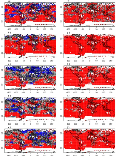
the sub-periods of 250 records. For example, SIM is con-sistent with the target in the North Atlantic sub-polar gyre region for the early sub-period (about 800 to 1050, Fig. 10b) but not for the following one (Fig. 10c). Overall, opposite results are common in the full test for these early two pe-riods. SIM is consistent with the target over wide regions
−150 −100 −50 0 50 100 150
−50
0
50
a)
Latitude[3:34]
−150 −100 −50 0 50 100 150
−50
0
50
f)
Latitude[3:34]
−150 −100 −50 0 50 100 150
−50
0
50
b )
Latitude[3:34]
−150 −100 −50 0 50 100 150
−50
0
50
g )
Latitude[3:34]
−150 −100 −50 0 50 100 150
−50
0
50
c )
Latitude[3:34]
−150 −100 −50 0 50 100 150
−50
0
50
h )
Latitude[3:34]
−150 −100 −50 0 50 100 150
−50
0
50
d )
Latitude[3:34]
−150 −100 −50 0 50 100 150
−50
0
50
i )
Latitude[3:34]
−150 −100 −50 0 50 100 150
−50
0
50
e )
Latitude[3:34]
−150 −100 −50 0 50 100 150
−50
0
50
j )
Latitude[3:34]
Fig. 10. Global assessment of the goodness-of-fit test for the decadal smooth data considering uncertainties in the target. Plotted are lower pvalues. In the left column: fullχ2test, in the right column: maximum ofpvalues for single deviation tests for bias and spread. Blue for smaller than 0.1, dark to light grey in steps of 0.2 for the range between 0.1 and 0.9, red for larger than 0.9. (a, f) full period and (b–e) and (g–j) for the first, second, third and last period of 250 records.
test again suggests that the SIM ensemble is consistent with the target over Eurasia and the North Atlantic according to the full test. On the other hand, single deviations are nearly always and everywhere significant (Fig. 10f–j). Deviations
target-uncertainties, we again find notable probabilistic over-dispersion (not shown) and also the climatological assess-ment indicates general over-dispersion (not shown).
In summary, even more prominent than for the area-averaged time series, the SIM ensemble displays a lack of consistency with its target for decadally smoothed global temperature field data. The different diagnosed biased, under- and over-dispersive discrepancies suggest that the re-lations between ensemble and target differ strongly in differ-ent regions. However, we cannot reject a uniform outcome of the rank counts for some regions and certain periods based on the full test. This may be to some extent due to a very small number of independent samples. Lack of consistency is most prominent over the southern oceans. Tests for the single de-viations of bias and spread are nearly everywhere significant. Thus general consistency between the SIM ensemble and its field data target remains very weak. Note that the (lack of) consistency is not homogeneous in time, but may differ be-tween selected periods. It is not necessarily valid to assume an increase in consistency with decreasing temporal distance to the present.
3.2.2 Addressing lack of consistency in spatial fields
Figure 7a presented the reconstructed mean anomaly map for an arbitrary sub-period (1390s to 1690s) encompassing part of the Little Ice Age (LIA). The LIA was chosen as it depicts one period of special interest in the literature. This period is only partially captured in the previous assessments of consis-tency. However, Fig. 10 indicates that we cannot expect too many differences between the considered sub-periods and this partially independent one. Based on Fig. 7, we are go-ing to trace possible sources of lack of consistency.
The reconstructed estimate basically fully relies on a sta-tistical relation between observations and the proxies. The simulated estimate relies on our knowledge on the physics of the climate system as coded in the simulator.
We note that the amplitudes of mean anomalies are compa-rable between reconstructions and SSIM simulations except in the tropical Pacific, but the WSIM ensemble members dis-play less cooling in the selected period (not shown, compare reconstruction in Fig. 7a, SIM ensemble mean in Fig. 7b and rank map in Fig. 7d). Mapped ranks in Fig. 7d exemplify the potential differences in simulated and reconstructed mean anomaly patterns. Obviously, there are large discrepancies between both approaches as highlighted by the cold bias of the SIM ensemble in the tropical Pacific and further spatially extended biases in most oceanic regions. SIM is biased low over the tropical Pacific ocean but a high bias is seen over most other oceanic regions, North America and eastern and western Eurasia. These biases are not representative for the full period as we discuss above (compare Fig. 10). Rather, Fig. 7c highlights how strongly mean anomalies of SIM may disagree with the target patterns for specific periods.
On the other hand, variability is often regionally compara-ble over the full period of the data (compare the ensemcompara-ble- ensemble-mean relative standard deviations in Fig. 7c) but also over sub-periods (not shown). Nevertheless, the reconstructed variability is strongly overestimated in the South Atlantic or more generally southern hemispheric ocean regions. Simi-larly, the SIM members often display more variability than the target over the other oceanic regions (see Fig. 7c). Sub-periods give comparable patterns, but slight changes may of course be found in the specific size of over or underestima-tion of variaunderestima-tions. Differences in variability between target and ensemble are rather small-scale over the continents. The rank counts in Fig. 8 reflect these regional differences in vari-ability. For instance, grid points in the southern hemispheric Atlantic sector suggest opposite biases in different periods, while, for the mid- to high-latitude North Pacific grid points, they suggest largest over-dispersion for the model-ensemble. The mapped ranks (Fig. 7d) highlight another feature that also appears in other sub-periods and even for some further field reconstructions (not shown): the reconstruction target generally represents the largest absolute mean anomalies in the set of SIM ensemble and target.
Thus reconstructions and simulations commonly differ in the mean and in the variability for certain periods. The SIM ensemble generally underestimates the size of the mean anomalies with reconstructed warm anomalies being warmest and cold anomalies coldest, which results in en-semble biases. Further, the enen-semble members vary more strongly in the averaging periods, which leads to common over-dispersive relations. The latter feature is amplified in the analyses of consistency by considering the uncertainty of the target. The underestimating biases possibly relate to general differences in the long-term trend between the en-semble members and the target field reconstruction. These, in turn, are spatially explicit expressions of the differences in the long-term tendencies that were similarly found in the large-scale mean data (compare Figs. 2 and 3). Franke et al. (2013) report a general overestimation of low-frequency vari-ability in proxies and reconstructions. This, in turn, possibly explains our finding of more variability in the simulations, also on the decadal scale, compared to the reconstruction.
Both, differences in trend and in variability, express a gen-eral misrepresentation of the climate statistics. Therefore, comparing anomaly patterns is of reduced value due to a general dissimilarity between reconstructions and simula-tions. Thus the assessment of ensemble consistency not only reduces the subjectivity of a comparison between simula-tions and reconstrucsimula-tions but, in turn, may help in clarifying sources of disagreement in the statistics.
4 Discussions of the results
long-term trends before applying tests of consistency (simi-lar to traditional simulation-reconstruction comparisons, e.g. Jansen et al., 2007; Br´azdil et al., 2010; Luterbacher et al., 2010; Jungclaus et al., 2010; Zorita et al., 2010; Zanchettin et al., 2013). For instance, Jungclaus et al. (2010) show good agreement between the full-forcing simulations in the COSMOS-Mill ensemble and the HadCRUT3v Northern Hemisphere temperature data for the 20th century. They also highlight periods in which the simulations are rather warm compared to temperature reconstructions when temperature deviations are considered with respect to the period 1961– 1990 (e.g. in the 12th and 13th centuries). We accept that the choice of the reference period influences the results.
Strong probabilistic and climatological deviations arise, in some cases, between the considered ensembles of simula-tions and reconstrucsimula-tions for the hemispheric data. Results are to some extent dependent on the utilized uncertainty es-timates and the reference periods. For the Northern Hemi-sphere data, the choice of the specific sub-ensemble also has an influence. The simulation ensemble is also generally over-dispersive for the seasonal European temperature recon-structions by Luterbacher et al. (2002, 2004) and Xoplaki et al. (2005) or the South American austral summer temper-ature reconstructions by Neukom et al. (2011) as targets (not shown). Even if the ensemble is consistent according to our analyses at the grid-point level or for area-averaged index-series, the associated uncertainties usually lessen the value of such consistency. Only the annual Central European tem-perature time series data arises as fully consistent between the simulation ensemble and the reconstruction. Thus the SIM ensemble is only consistent with an estimate for the last 500 yr and, therefore, may benefit from a more stable number of reliable available proxy indicators compared to longer pe-riod reconstructions. The forcing data used to drive the simu-lations can also be assumed to be less uncertain in this shorter period compared to the full millennium. However, part of the large simulated climate variability is possibly due to the well known too strong and too regular El Ni˜no variability and the related teleconnections in the considered climate simulator (Jungclaus et al., 2006). On the other hand, Franke et al. (2013) highlight the general overestimation of low-frequency variability in proxies and reconstructions compared to obser-vations and simulations.
As noted in Sect. 2.3, it is convenient, but not necessar-ily appropriate, to employ the raw ensemble reconstructions by Frank et al. (2010) as representing inter-annual varia-tions. Similarly, it is arguable whether or not an ensemble mean represents inter-annual variability. Results change no-tably when uncertainties are included or excluded and/or when internal variability in the assessment of the FRS en-semble against the target of the SIM enen-semble mean is con-sidered. Although the temporal evolutions notably deviate, it appears likely that the FRS and most of its members are in-deed consistent with the target of the SIM ensemble mean under the assumptions made on internal variability and the
uncertainties. On the other hand, the SIM ensemble displays pronounced deviations from consistency relative to the target of the FRA ensemble mean including different estimates of internal variability. Interestingly, the moving standard devi-ations of the ensemble means (simuldevi-ations and reconstruc-tions) evolve to some extent similarly in the period 1400 to 1900 (compare Figs. 1–3). The 20th century disagreement is possibly due to the evolution of the simulations within the SSIM ensemble (i.e. with strong solar forcing). The consid-erations on internal variability introduce an additional source of uncertainty. While the consideration of internal variability reduces the problems in employing ensemble-mean targets, it also highlights the ambiguity of our estimates of past climate trajectories.
Sundberg et al. (2012) and Hind et al. (2012) provide a sta-tistical framework for assessing climate simulations against paleoclimate proxy reconstructions allowing for an irregu-lar spatiotemporal distribution of proxy series. Their goal is similar to the approach utilized here. Their framework fo-cuses on the similarity between simulated and reconstructed series by analysing two newly developed correlation-based and distance-based test statistics. Hind et al. (2012) apply their approach in a pseudo-proxy experiment within the vir-tual reality of the COSMOS-Mill sub-ensembles to assess the distinguishability of the two sub-ensembles. They conclude that prior to drawing resilient conclusions from our model simulations, we need more proxy series with high signal-to-noise ratios. We propose that, in parallel, we need to address the compatibility of reconstructions and simulations by eval-uating their probabilistic and climatological consistency un-der the paradigm of statistical indistinguishability.
Finally, the CMIP5/PMIP3 ensemble of past1000 simu-lations (Taylor et al., 2012; Braconnot et al., 2012) offers the opportunity to evaluate our simulated and reconstructed knowledge in a multi-model context. Similarly, the PAGES 2K Network (http://www.pages-igbp.org/) aims to provide new regional reconstructions for all continental areas and the global ocean. This also allows for a detailed assess-ment of the consistency between simulations and reconstruc-tions. Preliminary analyses for the available CMIP5/PMIP3-past1000 simulations indicate that, for the European and northern hemispheric temperature reconstructions consid-ered in the present study, the multi-model ensemble behaves similar to the COSMOS-Mill ensemble with respect to prob-abilistic and climatological consistency.
5 Concluding remarks
instrumental observations, such statistical analyses reduce the subjectivity in comparing simulation ensembles and sta-tistical approximations from paleo-sensor data (Braconnot et al., 2012) under uncertainty and go beyond “wiggle match-ing”. The approach permits a succinct visualization of the consistency between an ensemble of estimates and an un-certain verification target. Ideally, it also reduces the depen-dence on the reference climatology which is present in many visual and mathematical methods that aim to qualify the cor-respondence between simulations and (approximated) obser-vations.
We considered the COSMOS-Mill ensemble (Jungclaus et al., 2010) and various reconstructions within the described approach. We found the simulation ensemble to be consis-tent, within samplin