https://doi.org/10.5194/amt-11-4963-2018 © Author(s) 2018. This work is distributed under the Creative Commons Attribution 4.0 License.
Clutter mitigation, multiple peaks, and high-order spectral
moments in 35 GHz vertically pointing radar velocity spectra
Christopher R. Williams1, Maximilian Maahn2,3, Joseph C. Hardin4, and Gijs de Boer2,3
1Ann and H. J. Smead Aerospace Engineering Sciences Department, University of Colorado Boulder,
Boulder, CO 80309, USA
2Cooperative Institute for Research in Environmental Science (CIRES), University of Colorado Boulder,
Boulder, CO 80309, USA
3NOAA Earth System Research Laboratory (ESRL), Physical Sciences Division, Boulder, CO 80305, USA 4Pacific Northwest National Laboratory (PNNL), Richland, WA 99354, USA
Correspondence:Christopher R. Williams ([email protected]) Received: 27 February 2018 – Discussion started: 17 April 2018
Revised: 2 August 2018 – Accepted: 11 August 2018 – Published: 3 September 2018
Abstract. This study presents and applies three separate processing methods to improve high-order moments esti-mated from 35 GHz (Ka band) vertically pointing radar Doppler velocity spectra. The first processing method re-moves Doppler-shifted ground clutter from spectra collected by a US Department of Energy (DOE) Atmospheric Radi-ation Measurement (ARM) program Ka-band zenith point-ing radar (KAZR) deployed at Oliktok Point (OLI), Alaska. Ground clutter resulted from multiple pathways through antenna side lobes and reflections off a rotating scanning radar antenna located 2 m away from KAZR, which caused Doppler shifts in ground clutter returns from stationary tar-gets 2.5 km away. After removing clutter in the recorded ve-locity spectra, the second processing method identifies multi-ple separate and sub-peaks in the spectra and estimates high-order moments for each peak. Multiple peaks and high-high-order moments were estimated for both original 2 and 15 s aver-aged spectra. The third processing step improves the spec-trum variance, skewness, and kurtosis estimates by removing velocity variability due to turbulent broadening during 15 s averaging intervals.
Applying the multiple peak processing to Doppler veloc-ity spectra during liquid-only clouds can identify cloud and drizzle particles and during mixed-phase clouds can identify liquid cloud and frozen hydrometeors. Consistent with pre-vious studies, this work found that spectrum skewness as-suming only a single spectral peak was a good indicator of two hydrometeor populations (for example, cloud and drizzle
particles) being present in the radar pulse volume. Yet, after dividing the spectrum into multiple peaks, velocity spectrum skewness for individual peaks is near zero, indicating nearly symmetric peaks. This suggests that future studies should use velocity skewness of single-peak spectra as an indicator of possible multiple hydrometeor populations and then use multiple-peak moments for quantitative studies. Three future activities will continue this work. First, KAZR spectra from several ARM sites have been processed and are available in the ARM archive as a principal investigator (PI) product. ARM programmers are evaluating these processing methods as part of future multiple-peak products generated by ARM. Third, MATLAB code generating the Oliktok Point products has been uploaded as supplemental material for public dis-semination.
1 Introduction
contain microphysical and dynamical cloud and precipitation information.
Using narrow-beam-width antennas reduces spectrum broadening due to sub-pulse volume turbulence. The result-ing recorded spectra are often non-Gaussian shaped and con-tain multiple peaks due to the presence of different parti-cle size distributions within the radar pulse volume (Kollias et al., 2016). Under certain atmospheric conditions, mixed-phase clouds occur and contain both liquid- and ice-mixed-phase particles within the same radar pulse volume (Shupe et al., 2004; Kalesse et al., 2016). Thus, the number of spectrum peaks and their shape provide microphysical information of the particle size distributions. Estimating higher-order spec-tral moments, including velocity spectrum skewness and kurtosis, extracts microphysical information from the full Doppler spectrum (Luke and Kollias, 2013). These high-order moments are inputs to time–height analyses explor-ing microphysical and dynamical cloud processes (Maahn and Löhnert, 2017). One caveat for this analysis paradigm is the need for clean radar Doppler velocity spectra void of non-atmospheric signals, including ground clutter. Thus, pre-processing and cleaning of Doppler spectra are often needed before microphysical and dynamical information can be ex-tracted from vertically pointing cloud radar observations.
This study presents three separate methods to improve high-order moments estimated from Doppler spectra. First, Doppler velocity spectra are cleaned by removing ground clutter. Second, multiple peaks are identified within the Doppler spectra. Finally, spectrum skewness estimates are improved by removing turbulent broadening effects at the 15 s scale.
Ground clutter in scanning and vertically pointing radar observations is a pervasive problem (Sato and Woodman, 1982). Ground structures (including buildings, trees, and power lines) act as hard targets reflecting radar waves back to the radar. Since these ground structures are stationary, except for oscillatory trees and power lines swaying due to wind (Barth et al., 1994), the ground clutter has a zero Doppler ve-locity shift. Bandpass filters can isolate clutter and hydrom-eteor signals as long as the hydromhydrom-eteor signal has a non-zero velocity. As the weather signal approaches non-zero veloc-ity, more sophisticated methodologies are needed to separate clutter from desired weather signals (Siggia and Passarelli, 2004).
For scanning weather radars, both the clutter and weather signals have Gaussian shape peaks that enables removing the clutter signal and recovering any overlapping weather signal. Within the Doppler velocity spectrum domain, the Gaussian model adaptive processing (GMAP) method (Siggia and Pas-sarelli, 2004) uses the saved coherent and quadrature time-series observations (i.e., I and Q voltages) to calculate multi-ple spectra to adaptively determine the Gaussian-shaped clut-ter and remove it from the Gaussian-shaped weather signal. The GMAP methodology applied to time-domain calcula-tions (called GMAP-TD) accounts for scanning radars
utiliz-ing staggered pulse repetition time (PRT) sequences (Nguyen and Chandrasekar, 2013). Since vertically pointing radars in mixed-phased clouds routinely observe signals from two hy-drometeor types (e.g., liquid clouds and falling ice particles, Shupe et al., 2004; Kalesse et al., 2016), the GMAP method cannot be implemented to remove clutter without signifi-cantly modifying the GMAP logic. In addition, the time-series I and Q voltages needed to resample the spectra with different amplitude weightings are often not available for re-analysis from vertically pointing radars.
Receiving backscattered energy from moving trees and cars through antenna side lobes is a common clutter problem with wind profilers (Barth et al., 1994). Due to the relatively large antenna beam widths in wind profilers (e.g., 6◦to 9◦ for main beams and larger for side lobes), clutter tends to be broad Gaussian-shaped features near zero velocity (May and Strauch, 1998). Birds and bats are often detected in higher-frequency wind profilers (e.g., 915 MHz) with wavelet trans-forms and time-domain Gabor transtrans-forms being effective in identifying and removing these short-time duration targets (Jordan et al., 1997; Lehmann, 2012). In addition, the Gabor transform technique has been shown to improve wind pro-filer horizontal wind estimates (Bianco et al., 2013). Note that clutter is dependent on the radar operating frequency. For example, longer wavelength radars (e.g., VHF) are not as susceptible to clutter from flying birds as shorter wavelength 915 MHz wind profilers (Wilczak et al., 1995). In contrast to wind profilers, Ka-band cloud radars have significantly higher frequencies and very narrow beam widths (on the or-der of 0.3◦) such that Doppler velocity spectrum broadening due to horizontal motion through the radar beam is negligi-ble (Shupe et al., 2008; Kollias et al., 2007). These narrow beam widths result in very narrow clutter peaks in the Ka-band cloud radar velocity spectra with insects appearing as very narrow spectral peaks (Luke et al., 2008).
Recent studies have shown that velocity spectrum skew-ness provides information of drizzle onset (Kollias et al., 2011; Luke and Kollias, 2013; Acquistapace et al., 2017) and for deriving properties of ice clouds (Maahn et al., 2015; Maahn and Löhnert, 2017). Since there is a trade-off between temporal resolution and spectrum noise variance, the spectral moment estimates tend to be noisy for short-duration spec-tra (Giangrande et al., 2001; Luke and Kollias, 2013; Ac-quistapace et al., 2017). By shifting spectra to a reference velocity before averaging spectra, Luke and Kollias (2013) showed that spectrum skewness estimates improved and were more coherent in time and height.
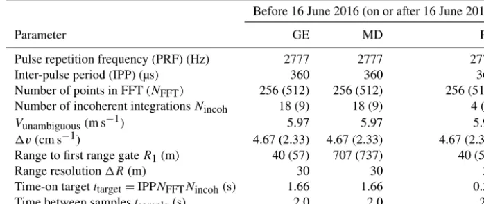
Table 1.Operating parameters for AMF-3 KAZR deployed at Oliktok Point, Alaska, from 1 October 2015 through 31 October 2017 (at the time of publishing, the radar was still operating at Oliktok Point, Alaska). Operating modes included general purpose (GE), medium sensitivity (MD), and precipitation (PR) modes. Tabulated parameters include pulse repetition frequency (PRF) (Hz), inter-pulse period (IPP) (µs), number of points in fast Fourier transform (FFT) (NFFT), number of averaged spectra (also known as number of incoherent
integrations) (Nave), unambiguous velocity (Vunambiguous) (m s−1), velocity resolution (1v) (m s−1), range to first range gate (m), range
resolution (m), time-on target (which is calculated using IPPNFFTNave) (s), and time between samples (s). Radar operating modes changed
on 16 June 2016 at 14:00 UTC. A clutter screen was installed on the antenna on 27 August 2016.
Before 16 June 2016 (on or after 16 June 2016)
Parameter GE MD PR
Pulse repetition frequency (PRF) (Hz) 2777 2777 2777 Inter-pulse period (IPP) (µs) 360 360 360 Number of points in FFT (NFFT) 256 (512) 256 (512) 256 (512)
Number of incoherent integrationsNincoh 18 (9) 18 (9) 4 (2)
Vunambiguous(m s−1) 5.97 5.97 5.97
1v(cm s−1) 4.67 (2.33) 4.67 (2.33) 4.67 (2.33) Range to first range gateR1(m) 40 (57) 707 (737) 40 (57)
Range resolution1R(m) 30 30 30 Time-on targetttarget=IPPNFFTNincoh(s) 1.66 1.66 0.37
Time between samplestsample(s) 2.0 2.0 2.0
or feature extraction, that can be used as input to algorithms that estimate boundary layer heights (Allabakash et al., 2017) or horizontal winds (Liu et al., 2017).
This paper has the following structure. Section 2 de-scribes the radar deployment and operating parameters of a US Department of Energy (DOE) Atmospheric Radia-tion Measurement (ARM) program Ka-band zenith pointing radar (KAZR) installed at Oliktok Point (OLI), Alaska. Sec-tion 3 describes signatures of clutter and atmospheric sig-nals observed in KAZR velocity spectra. Section 4 develops a clutter identification and mitigation method. This section also discusses how multipath scattering from a nearby scan-ning radar antenna caused the clutter to have either approach-ing or recedapproach-ing radial motion. Section 5 describes a method to identify multiple peaks in the spectra and estimate high-order spectral moments. Section 5 also discusses a method of shifting individual spectra to the 15 s mean velocity before averaging. Section 6 provides concluding remarks. For com-pleteness and repeatability, Appendix A provides the equa-tions to estimate high-order spectral moments. The MAT-LAB code used to perform the analysis is available as sup-plemental material.
2 Radar observations
Since the early 1990s, the US Department of Energy (DOE) Atmospheric Radiation Measurement program has deployed atmospheric observing systems around the globe to measure and characterize the radiative properties of the atmosphere (Mather and Voyles, 2013). The radiative properties of clouds are dependent on many factors including cloud composition, cloud thickness, and temperature. Measurements from
ver-tically pointing cloud radars, lidars, and radiometers provide the input observations needed to estimate and to better model the radiative properties of clouds (Clothiaux et al., 2000).
In 2015, DOE installed their third ARM Mobile Facil-ity (AMF-3) at Oliktok Point, on the North Slope of Alaska (NSA), which is approximately 264 km east-southeast of the long-term ARM North Slope of Alaska core-observing site near Utqia˙gvik (formally known as Barrow). The AMF-3 instrument suite includes a Ka-band (35 GHz) ARM zenith pointing radar (KAZR) and a Ka/W-band (35/94 GHz) scan-ning ARM cloud radar (SACR, until September 2017). Both antennas are installed on top of the same shipping sea con-tainer as shown in Fig. 1. The SACR antennas are less than 2 m from the KAZR antenna with a direct line of sight to the KAZR feed horn. As will be investigated in Sect. 3, the rotating SACR antennas are in the KAZR near-field, which caused the stationary ground clutter targets to be Doppler shifted alternating between approaching and receding.
The KAZR and SACR at Oliktok Point became opera-tional after an intensive calibration, grooming, and align-ment (CGA) field campaign conducted by the ARM Radar Engineering Group in October 2015. The KAZR operates in three modes: general mode (GE), medium mode (MD), and precipitation mode (PR). The initial operating pa-rameters recorded 256-point Doppler velocity spectra. On 16 June 2016, the number of incoherent integrations were reduced in order to record 512-point spectra and maintain the same time-on target (Table 1). Raw spectra used in this study are available on the DOE ARM archive (ARM Climate Research Facility, 2015).
Figure 1. (a)Photo of AMF-3 Ka/W-band scanning ARM cloud radar (Ka/W-SACR) antennas (left) and Ka-band ARM zenith radar (KAZR) antenna (right) as deployed at Oliktok Point, Alaska (photo credit: Gijs de Boer).(b)Photo of clutter screen mounted around KAZR antenna with snow on the KAZR radome (photo credit: Joe Hardin).
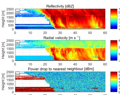
Figure 2. Time–height cross sections of original KAZR Doppler velocity spectral moments and attributes from 19 June 2016 during hour 12:00 UTC.(a)Reflectivity (dBZ),(b)mean radial velocity of dominant single peak (m s−1) (positive values are approaching the radar), and(c)maximum power drop from peak magnitude to either nearest neighbour (dBm). At least three consecutive spectral points needed to be above the noise threshold before estimating the moments. Large power drop from peak to nearest neighbour is an indicator that clutter peak was selected as the dominant peak.
the radar system through antenna side lobes. To mitigate the ground clutter observed in the KAZR spectra, a tem-porary clutter screen was installed around the KAZR an-tenna on 27 August 2016 (Fig. 1b). Thus, there are three different KAZR configurations partitioned by date: (prior to 16 June 2016) 256-point spectra with no clutter screen, (be-tween 16 June 2016 and 26 August 2016) 512-point spectra with no clutter screen, and (after 26 August 2017) 512-point spectra with clutter screen.
3 Atmospheric and non-atmospheric signal signatures Stationary ground clutter will appear in the Doppler velocity spectra near zero velocity. This section examines and quanti-fies the characteristics, or signatures, of KAZR ground clut-ter and KAZR atmospheric signals due to clouds and precip-itating particles. Appendix A provides details of calculating spectral moments from raw velocity spectra.
3.1 Ground clutter contamination
Figure 2 shows time–height cross sections of measured radar reflectivity (Fig. 2a) and mean radial velocity (Fig. 2b, pos-itive values are approaching the radar) for 1 h of observa-tions starting at 12:00 UTC on 19 June 2016. For this fig-ure, instead of imposing a user-defined signal-to-noise ra-tio (SNR) threshold to discriminate spectra with signal-plus-noise versus spectra with just signal-plus-noise, moments were estimated only for spectra containing at least three consecutive spectral points above the noise threshold. While the actual observa-tions for this precipitation event extend above 6000 m, the vertical axis in Fig. 2 is limited to 2500 m to show details of the ground clutter signatures. There are four general ar-eas of interest in this figure: one area contains atmospheric signals and the other three areas contain clutter signatures. The atmospheric signals are due to cloud and precipitating particles that are identifiable by reflectivities greater than ap-proximately−10 dBZ and downward velocities greater than 1 m s−1reaching the surface after minute 25. There is also a
bright band in reflectivity near 1500 m and a large gradient in downward motion near 1500 m indicating the melting of ice particles into raindrops (e.g., Williams et al., 1995).
clutter within these two height ranges throughout the hour. The clutter signature is not visible after minute 20 because signal power from the cloud and precipitation is larger than the clutter power and the spectral-peak-picking routine is se-lecting the larger atmospheric peak. At a height near 500 m and minutes 30–60, there are intervals when the clutter peak is larger than the atmospheric peak such that the spectral-peak-picking routine has selected the clutter peak instead of the atmospheric peak. These clutter peaks appear near min-utes 31 and 50–57 and are distinguished by discontinuities in reflectivity and near-zero radial velocities.
3.2 Drop in power from peak to nearest neighbour There are significant differences in the characteristics of backscattered return power from distributed targets and from point targets (Mahafza, 2017). In the case of distributed hy-drometeor targets, the hyhy-drometeors have different sizes and velocities that are constantly moving within the radar pulse volume. These motions cause the radar-received backscat-tered power to fluctuate from pulse to pulse (i.e., Swerling type II targets). In addition, there is a distribution of differ-ent particle sizes falling at differdiffer-ent velocities leading to a broad velocity distribution in the recorded Doppler velocity spectrum.
In contrast, received power return from stationary point targets is nearly constant from pulse to pulse with small ran-dom statistical fluctuations (i.e., Swerling type 0 or V tar-gets). The constant path length between the radar and the target results in zero Doppler motion. In an ideal signal-processing environment, the stationary target in the time do-main would transform into a delta function of finite energy at zero velocity in the frequency domain. However, in real-world signal processors, the delta-function energy spreads over several velocity bins following asincfunction. Thesinc function breadth and amplitude are determined by the win-dowing function applied to the time series before performing a fast Fourier transform and by the delta-function amplitude (Mafazha, 2017).
In general, distributed hydrometeor targets produce broader velocity spectra than stationary targets. To explore these attributes in the recorded spectra, Fig. 2c shows the drop in received power from the velocity bin with peak mag-nitude to its directly neighbouring velocity bin expressed in units of dBm (i.e., power relative to 1 mW). Since there are two neighbouring velocity bins bounding the peak value, all calculations use the largest power drop. Figure 2c shows that the power drop for the clutter signal is approximately 6 dBm (i.e., red colours) and occurs prior to minute 25, as well as near 500 m during minutes 31 and 51–57. For the spectra with clouds and precipitation, the drop in power is a distribu-tion of values with a central value near approximately 2 dBm (i.e., blue colours). Figure 2c suggests that the power drop from the peak magnitude to the nearest neighbour is a good indicator of whether the spectrum peak is due to point-target
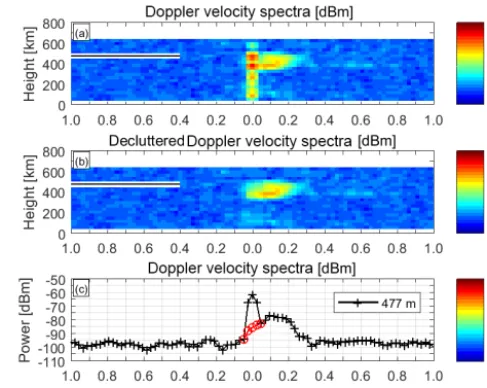
Figure 3. Doppler velocity spectra for profile collected on 19 June 2016 at 12:05:01 UTC.(a)Original Doppler velocity spec-tra at each range gate as a function of radial velocity.(b)Similar to panel(a), expected spectra were interpolated across DC (zero veloc-ity) to mitigate the clutter signal.(c)Original spectrum (black line and pluses) and decluttered spectral points (red line and circles) at 447 m range (black line inaandb).
scattering (approximately 6 dBm drop) or due to distributed hydrometeor target scattering (less than 2 dBm drop).
To explore details of how clutter signals appear in the recorded velocity spectra, Fig. 3a shows a profile of spec-tra selected from Fig. 2 at 12:05:01 UTC on 19 June 2016. The radial velocity is on the abscissa and only extends from 1 m s−1upward (left side) to 1 m s−1downward (right side).
The ordinate is height above the ground in metres and ex-tends from the surface up to 800 m. The pseudo-colours rep-resent received power in dBm. In nearly all range gates, ground clutter power is identifiable as an increase in received power at zero velocity with additional power leaking into neighbouring velocity bins.
The black line at 447 m in Fig. 3a indicates the height of the spectrum shown in Fig. 3c, which contains both a clutter peak and an atmospheric peak due to cloud droplet particles (black line with pluses). An interpolation in linear units is performed across the three points centred about zero veloc-ity and is shown in Fig. 3c with a red line and circles. It is important to note that the three-point interpolation only mod-ifies power recorded at three velocity bins. Figure 3b shows stacked spectra after applying this three-point interpolation to each spectrum. Note that this simple interpolation was suf-ficient to remove or suppress the clutter near zero velocity such that the atmospheric signal can be resolved.
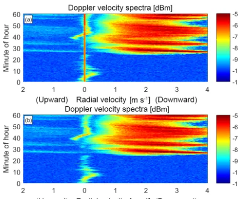
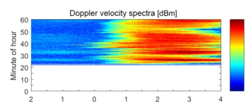
Figure 4.Time series of radial velocity spectra on 19 June 2016 during hour 12:00 UTC at 447 m range. The first spectrum of the hour is at the bottom of the panel (minute 0) and last spectrum of the hour is at the top of the panel (minute 60). Horizontal axis is upward (left side) and downward (right side) radial velocity.(a)Original spectra and(b)decluttered spectra.
is on the abscissa with upward motion on the left and down-ward motion on the right. Time is on the ordinate with time increasing up the page. Pseudo-colours represent measured return power in dBm. A clutter peak near zero velocity is present during the whole hour while there are two fluctu-ating atmospheric signals at this height. A liquid cloud is present for most of the hour with updraft–downdraft mag-nitudes less than 0.5 m s−1. After approximately minute 28, raindrops appear at this height with downward radial veloc-ities ranging from approximately 0.25 to over 4 m s−1. The small-magnitude power signals with upward motions after minute 28 are artefacts due to large-magnitude downward power signals causing harmonics in the radar receiver. Fig-ure 4b shows the spectra after applying the three-point in-terpolation across the zero velocity. This simple three-point interpolation is sufficient to remove the clutter peaks without disturbing the atmospheric signals.
4 Clutter identification and mitigation
As shown in Fig. 2 during the first 20 minutes of obser-vations, without clutter peak mitigation, standard single-peak-picking algorithms (e.g., Carter et al., 1995) will select ground clutter as a viable peak and will estimate the spec-tral moments of this clutter peak. If the clutter peak is in the middle of the atmospheric signal as in the example spec-trum shown in Fig. 3c, then the estimated reflectivity will be biased high and the mean radial velocity will be biased toward zero velocity. If clutter mitigation is applied to all
spectra regardless of whether clutter signals are present, then low-magnitude atmospheric signals centred on zero velocity could be eliminated from the dataset. Thus, this section ex-amines the power drop near zero velocity in order to establish a threshold to determine where and when not to apply clutter mitigation.
4.1 Clutter-to-noise ratio (CNR)
To determine whether the spectrum contains point-target signatures, three statistics are calculated for each spec-trum: the drop in power from the zero velocity bin to the nearest-neighbour velocity bin (Pdrop), the clutter-to-noise
ratio (CNR), and the signal-to-noise ratio (SNR) of the de-cluttered spectrum.Pdrop is a clutter indicator while CNR
quantifies the clutter power. Figure 5a shows a typical spec-trum containing clutter power near zero velocity, collected at 00:14:33 UTC on 4 July 2016 at range 387 m. While the recorded spectrum extends to upward and downward Nyquist velocities of 5.9 m s−1, this figure only shows radial ve-locities out to 0.4 m s−1. A peak power of approximately −60 dBm occurs at zero velocity andPdropis approximately
6 dB. The thick dashed line shows the three-point interpo-lation with the light grey shaded area indicating the clutter power. The dark shaded area represents noise power. The CNR is defined as the clutter power (light grey shaded area but expressed in linear units) divided by total noise power (dark grey shaded area extended to Nyquist velocities and expressed in linear units) with CNR expressed in decibel units (dB).
In Fig. 5a, notice the large power drops between the zero velocity bin and the first and second neighbouring velocity bins. The power drops are approximately 6 and 25 dBm, re-spectively. These large power drops are consistent with the expectedsincfunction from point targets. A large power drop to the second neighbouring bin is not always observed be-cause either (1) the spectrum power falls below the noise threshold or (2) the power drop is masked by an atmospheric signal power as in the case shown in Fig. 5c. In this dataset, the clutter peak was narrow enough that a three-point inter-polation removed clutter power from the peak value and two neighbouring velocity bins were sufficient to remove most of the clutter power. For other radar datasets, a three-point inter-polation may not be sufficient to remove the clutter. There-fore, the clutter characteristics in other datasets should be ex-amined before adjusting the width of the interpolation.
Figure 5. Selected spectra to illustrate clutter signal, three-point interpolation, and residual signal power.(a)Original spectrum from 4 July 2016 at 00:14:33 UTC at 387 m range with clutter power shaded in light grey.(b)Same spectrum as in(a)except for a three-point linear interpolation across zero velocity to remove clutter power with residual signal peak power shaded in medium grey colour. The noise power is shaded the darkest grey in all panels. Panels(c)and(d)are similar to panels(a)and(b)except spectra were collected on 7 July 2016 at 17:14:31 UTC. The solid circle in panels(b)and(d)indicates the velocity of the peak magnitude in the residual spectra. Due to this peak magnitude velocity, the residual signal in panels(b)and(d)is deemed residual clutter and atmospheric signal, respectively.
(indicated with a filled circle), and this velocity bin is called the “peak magnitude velocity”.
The spectrum shown in Fig. 5c contains both clutter and atmospheric signals (range 387 m at 17:14:31 UTC on 7 July 2016). The clutter peak is clearly identifiable in the spectrum. A thick dashed line shows the three-point interpo-lation across zero velocity and the clutter power is shaded in light grey. Figure 5d shows the decluttered spectrum with the residual signal power and noise power indicated with the medium and dark grey shadings, respectively. For this spec-trum, the residual peak SNR is 3.3 dB and the peak magni-tude velocity (indicated with a filled circle) occurs away from the three-point interpolation velocity bins and is associated with the atmospheric signal.
In order to determine when to apply the three-point inter-polation across zero velocity, we need to compare the drop in power in spectra with and without ground clutter. Figure 6 shows a time series of radial velocity spectra at a range of 987 m for the same 1 h interval shown in Fig. 4a. There is no clutter in the raw spectra at 987 m shown in Fig. 6 so it can be used as a reference. Note that there are no saved spec-tra prior to minute 21 because the automated data reduction and archiving algorithm did not detect any spectral points (clutter or atmospheric signals) with power greater than the Hildebrand and Sekhon (1974) noise threshold.
The power drop from zero velocity to the nearest-neighbour Pdrop and CNR statistics were calculated for all
spectra shown in Fig. 6. Only 210 spectra had a positive power drop, with Fig. 7a showing a scatter plot of CNR vs. power drop (squares). The CNR vs. power drop for the
simul-Figure 6.Similar to Fig. 4a except for 987 m range. In contrast to the range gate at 447 m shown in Fig. 4, this range gate does not contain ground clutter for this hour and does not contain any atmospheric signal before minute 21. Since no signal was detected above the noise threshold before minute 21, the data reduction and storage algorithm did not save any spectra before minute 21.
dif-Figure 7. (a)Scatter plot of clutter-to-noise ratio (CNR) vs. power dropPdropfrom zero velocity to nearest neighbour for the same profiles at ranges 477 m (circles) and 987 m (squares) for hour 12 of 19 June 2016. Spectra at 477 m contained clutter and spectra at 987 m did not have clutter.(b)Cumulative distribution function (CDF) of power drop for estimates shown in(a). These estimates were derived from spectra shown in Figs. 4a and 6. There are 210 simultaneous samples during this rain event.
ferent for different datasets. To help determine appropriate thresholds in other radar datasets, the MATLAB code used in this study is available in the Supplement.
4.2 Ground clutter Doppler shift
Time–height clutter patterns occurred with a repeatable tem-poral cadence. Specifically, there were periods of narrow-symmetric clutter and periods of broader-anarrow-symmetric clutter. While the peak magnitude velocity rarely deviated from zero velocity, the asymmetry caused the mean velocity moment to deviate from zero velocity. Figure 8 shows an hour’s worth of observations on 3 July 2016 (hour 20:00 UTC) when no hy-drometeors were above the radar. Figure 8a shows the clutter-to-noise ratio (dB), Fig. 8b shows the residual peak SNR (dB), and Fig. 8c shows the residual peak magnitude veloc-ity expressed in m s−1. Note that the peak magnitude veloc-ity alternates between negative and positive radial velocities, suggesting that the stationary ground clutter has a Doppler motion component and is either receding or approaching the radar, respectively.
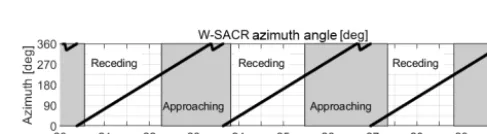
Figure 9 shows the pointing direction of the SACR scan-ning radar antennas (solid line) for minutes 20–30 during hour 20:00 UTC on 3 July 2016. During this 10 min inter-val, the SACR antennas were rotating at 2◦min−1in a clock-wise direction. The white and grey shading in Fig. 9 rep-resents the column median residual peak magnitude veloc-ity estimated from Fig. 8c and is either receding (white) or
Figure 8.Time–height cross section of clutter statistics from spec-tra collected on 3 July 2016 during hour 20:00 UTC.(a) Clutter-to-noise ratio (CNR) based on clutter power from three points centred around zero velocity (see Fig. 6),(b)signal-to-noise ratio of resid-ual peak after removing clutter peak, and(c)velocity of spectral peak in the residual spectrum indicates a skewness of the residual peak. Positive peak velocities correspond to targets approaching the radar.
Figure 9.Diagram showing SACR antenna azimuth pointing di-rection (solid line) and Doppler shift of residual clutter (shading) for 10 min of observations shown in Fig. 7. With a rotation rate of 2◦min−1, the Ka/W-SACR antenna completed a rotation every 3 min. The residual clutter Doppler shift contained two phases per rotation indicating the antennas receding and approaching.
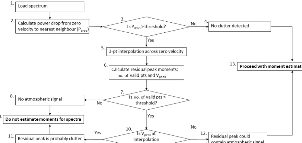
Figure 10.Clutter identification and mitigation flow diagram. Processing is performed on individual spectra without knowledge of clutter being identified in neighbouring spectra.
4.3 Clutter mitigation logic diagram
This section describes a clutter mitigation routine that iden-tifies and removes static and non-static clutter signals from recorded velocity spectra. Over the course of analysing clut-ter signatures, several complex clutclut-ter removal routines were developed. After comparing the results from these routines, the clutter removal methodology was simplified until this fi-nal routine had only three conditions based on two thresh-olds:
– Is powerPdropgreater than a threshold?
– Are there enough spectral points above the noise thresh-old to estimate moments?
– After interpolating across the clutter peak, is the new peak magnitude velocity at an interpolation edge veloc-ity?
The use of static thresholds is simple to implement, but not easily transferred to other radar systems that have different clutter statistics. Thus, the MATLAB code used to process the Oliktok Point KAZR dataset is made available as sup-plemental material. Figure 10 shows a flow diagram for the clutter mitigation routine. Starting with box no. 1, a single spectrum is loaded into the routine. The power drop from zero velocity to the nearest neighbour is calculated asPdrop
(box no. 2). If Pdrop is greater than a threshold as derived
from Fig. 7b (box no. 3), then this spectrum is flagged to contain clutter and passed to box no. 5; else, this spectrum does not contain clutter (box no. 4) and is saved for future
spectral and moment processing (box no. 13). If the spectrum gets into box no. 5, the three-point interpolation is performed across zero velocity and the residual moments are estimated in box no. 6.
anal-Table 2.Attributes and integration limits for three spectral peak regimes: single peak, sub-peak, and separate peak. All spectral peaks need at least five consecutive spectral points with magnitudes greater than the noise threshold (Hildebrand and Sekhon, 1974).
Peak name Attributes Integration limits
Single peak Contains the largest magnitude spectral point Determined by noise threshold (every valid spectrum has a single peak)
Sub-peak Sub-peaks are within integration limits of the single peak Determined by noise threshold or
determined by valley of at least 6 dB between sub-peaks Separate peak There are spectrum points below the noise threshold Determined by noise threshold
separating this peak from the single peak
Figure 11. Similar to Fig. 2 except spectra were decluttered (see Sect. 3) before estimating(a)reflectivity,(b)mean radial velocity, and(c)power drop from peak power to nearest neighbour.
ysis (box no. 9). If the peak magnitude velocity is different from either three-point interpolation edge velocity, then this spectrum likely contains an atmospheric signal (box no. 12) and is saved for future spectral and moment estimations (box no. 13).
To illustrate the performance of the clutter identification and mitigation routine, the same spectra used to construct Fig. 2 were processed through the flow diagram shown in Fig. 10. Figure 11 shows the decluttered spectra calculations of reflectivity (Fig. 11a), mean radial velocity (Fig. 11b), and power drop from peak power to nearest neighbour (Fig. 11c). Figure 11 shows a vertically thin cloud layer just below 500 m that was not visible in Fig. 2 because of the contami-nating ground clutter. This is consistent with the spectra anal-ysis shown in Figs. 3 and 4 that showed an oscillatory cloud layer near 500 m. In addition to providing the MATLAB code as supplemental material, the processed Oliktok Point KAZR datasets are available on the ARM archive (see data
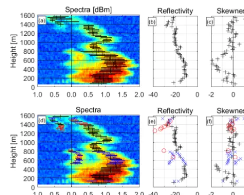
availabil-Figure 12.Profile of spectra and moments collected on 15 Octo-ber 2016 at 11:55:55 UTC. Top row corresponds to single-peak mo-ments and bottom row corresponds to multiple-peak momo-ments. Top row:(a)pseudo-colour represent spectral power (dBm) with mean velocity shown with black pluses and±spectrum bread shown with black lines,(b)reflectivity, and(c)velocity skewness. Bottom row: similar to the top row, except blue symbols represent sub-peaks and red symbols represent separate peaks.
ity section for details). These netCDF datasets also include a 3×3 time–height continuity filter quality flag so that the user can choose to remove isolated pixels (see Appendix B for details).
5.1 Identifying multiple peaks
One advantage of processing radar velocity spectra is that different hydrometeor habits can be identified by their veloc-ity signatures. For example, Fig. 12a shows a velocveloc-ity spectra profile when both cloud particles and ice particles are occur-ring in the same height between 500 and 800 m. This profile was collected on 15 October 2016 at 11:55:55 UTC with the pseudo-colours representing received power in dBm. Visu-ally, we can see two return power patterns in the spectra pro-file. One pattern is limited in height between 500 and 800 m and has downward motions between 0 and 0.4 m s−1that cor-respond to signals from cloud particles. Another return sig-nal extends from the top of the panel to the surface with downward motions ranging from 0 to 2 m s−1. While more analysis is needed to determine whether these return signals are from liquid- or ice-phase particles – e.g., cross-polarized spectra could provide linear depolarization ratio (LDR) esti-mates to discriminate spherical (likely liquid) particles from non-spherical particles – we can confidentially state that faster falling particles are larger than the cloud particles that are confined to the 500 to 800 m range.
Super imposed on the spectra in Fig. 12a are the mean ve-locityVmean(black vertical ticks) and±1 velocity spectrum
standard deviationVsig(horizontal black lines) estimated
as-suming that one spectral peak exists in each spectrum (see Appendix A for spectrum moment equations). These mo-ments are known as “single-peak” momo-ments and have a long lineage in vertically pointing radar research (see Carter et al., 1995) and the DOE ARM community (see Clothiaux et al., 2000). We can see that the single-peak moments do not rep-resent the dual-peak nature of the recorded spectra. To over-come this limitation, multiple spectral peaks are identified withVmeanandVsig estimated for each peak and shown in
Fig. 12d. The black symbols are from single-peak moments while the blue and red symbols are from sub-peaks and sep-arate peaks identified in the spectra.
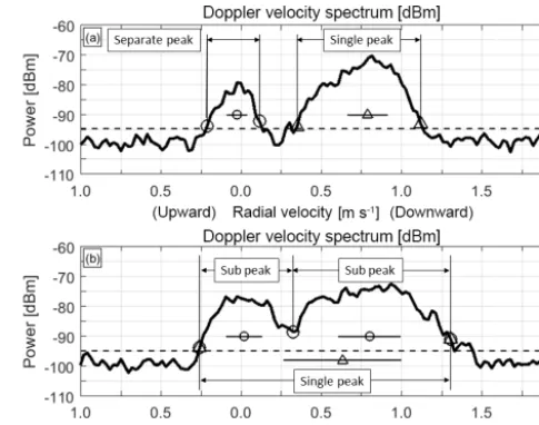
Identifying multiple peaks (Luke and Kollias, 2013) is a process of identifying boundaries, or integration limits, which will be used in the spectrum moment equations. To help describe how boundaries are identified, Fig. 13 shows how single peaks, sub-peaks, and separate peaks are identi-fied in example spectra pulled from heights 807 and 777 m in Fig. 12. Table 2 provides a description of the three types of peaks. Every spectrum with at least five consecutive spec-tral points above the noise threshold will have a single peak. However, not every spectrum with a single peak will have sub-peaks or separate peaks.
The spectrum from 807 m (Fig. 13a) has two spectral peaks. The peak on the right is the most significant peak be-cause it contains the spectral point with the largest magni-tude. The integration limits for the single peak extend over all consecutive points above the noise threshold. The triangles in Fig. 13a indicate the single-peak integration limits andVmean
andVsigare plotted near 0.8 m s−1downward velocity. Since
Figure 13. Radial velocity spectra on 15 October 2016 at 11:55:55 UTC at ranges(a)807 m and(b) 777 m. The spectrum in(a)contains two peaks separated with spectral power below the noise threshold. The single peak is the dominant peak due to the larger peak amplitude. The spectrum in(b)contains a single peak that spans from approximately 0.25 m s−1 upward to 1.3 m s−1 downward. This single peak contains two sub-peaks with a valley (or local minimum) near 0.3 m s−1downward.
there are spectral points below the noise threshold between the single peak and the left peak, the left peak is called a separate peak. Circles indicate the integration limits for this separate peak. The separate peak must have five consecutive spectral points above the noise threshold.
Figure 13b shows the spectrum from 777 m. The sin-gle peak is very broad and extends from approximately 0.25 m s−1upward to 1.3 m s−1downward as indicated with
the triangles. Sub-peaks are peaks within the single peak sep-arated by a local minimum, or valley. It is important that the valley is deeper than the bin-to-bin variability observed in the velocity spectrum. From Figs. 2 and 7, the variability from the peak magnitude value to the nearest neighbour exceeds 4 dB. Thus, this study used a valley threshold of at least 6 dB of concavity to limit the number of falsely identified peaks. The circles indicate the integration limits for two sub-peaks in Fig. 13b. TheVmean for all three peaks are shown
with triangles and circles, with±Vsigshown with lines.
Sim-ilar to the other peaks, sub-peaks must have five consecutive spectral points above the noise threshold.
5.2 High-order spectral moments
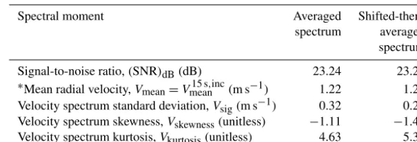
Table 3.Spectral moments of averaged spectrum after averaging eight spectra using two different methods. All eight spectra were collected during 15 s interval on 15 October 2016 between 11:55:45 and 11:56:00 UTC and are shown in Fig. 14. The averaged spectrum was con-structed by averaging individual spectra as shown in Fig. 14a. The mean radial velocity from this averaged spectrum is used as the reference velocity. The shifted-then-averaged spectrum was constructed by first shifting individual spectra to a reference mean radial velocity and then averaging as shown in Fig. 14b.
Spectral moment Averaged Shifted-then-spectrum averaged spectrum Signal-to-noise ratio,(SNR)dB(dB) 23.24 23.24
∗Mean radial velocity,
Vmean=Vmean15 s,inc(m s−1) 1.22 1.22
Velocity spectrum standard deviation,Vsig(m s−1) 0.32 0.28
Velocity spectrum skewness,Vskewness(unitless) −1.11 −1.44
Velocity spectrum kurtosis,Vkurtosis(unitless) 4.63 5.38
∗15 s averaged spectrum mean velocity used as reference velocity in the shifted-then-averaged procedure.
The scatter-plot profiles on the right side of Fig. 12 show the spectral moments of reflectivity and velocity skewness for the single, sub-, and separate peaks. The top row shows only the single-peak moments while the bottom row shows moments from different peaks. Note that if sub-peaks exist in a spectrum, then the single-peak moments are not plotted in the bottom row. The reflectivity vertical structure for the multiple peaks (Fig. 12e) shows both a continuous pattern with height and two patterns that are limited in height. The continuous pattern mimics the single-peak reflectivity pattern shown in Fig. 12b and has a local maximum near 400 m. The two height-limited patterns occur near 700 and 1400 m where there are two distinct hydrometeor populations in the spectra profile (Fig. 12d). Near 700 m, the smaller reflectivity values correspond to the cloud particles with mean velocities near 0.2 m s−1downward.
With regard to the velocity skewness, the single-peak es-timates (Fig. 12c) show large negative values below 800 m with maximum value near 600 m. A negative velocity skew-ness indicates that the long distribution tail is on the neg-ative velocity side of the peak, which is upward motion in this dataset. Yet, Fig. 12f shows near-zero velocity skewness for the sub-peaks between 500 and 800 m. This suggests that large-magnitude single-peak velocity skewness could indi-cate the existence of multiple sub-peaks. Yet, after identify-ing sub-peaks, velocity skewness represents the asymmetry of each individual spectral peak. Thus, single-peak velocity skewness could be used to identify the existence of multiple sub-peaks and moments from multiple peaks should be used to perform quantitative microphysical analyses.
5.3 Shift-then-average spectra
As discussed in Luke and Kollias (2013), the velocity spec-trum skewness can be a noisy estimator due to velocity bin-to-bin spectrum power fluctuations. To improve the velocity spectrum skewness estimate, Luke and Kollias (2013) sug-gested shifting consecutive spectra to a common reference,
averaging the shifted spectra, and then estimating the veloc-ity spectrum variance and skewness. Shifting the spectra be-fore averaging reduces the spectrum broadening and smear-ing due to vertical air motion variability that occurs dursmear-ing the averaging interval (Giangrande et al., 2001). Several dif-ferent averaging intervals were tested ranging from 4 s (sim-ilar the KAZR-ARSCL resolution) to 60 s. The 4 s interval only contained two profiles, while the cloud system often evolved and changed shape during the 60 s interval. A com-promise of 15 s is used assuming that the atmospheric mi-crophysical processes (e.g., evaporation, breakup, and coa-lescence) are stationary over this interval, yet dynamical pro-cesses (e.g., air motions and turbulence) are not stationary.
The method of shifting all spectra to line up all peak mag-nitude velocities appeared to work well for the maritime driz-zle clouds (Luke and Kollias, 2013), but it did not work well with Arctic mixed-phase clouds observed at Oliktok Point because the peak magnitude sometimes jumped to a different spectral peak during the 15 s integration interval. To over-come this occasional issue, the spectra were shifted to the 15 s mean velocity. Specifically, shift-then-average process-ing consisted of nine steps performed at each range gate:
1. Estimate the single-peak mean velocity for each 2 s spectrumVmean2 s .
2. Incoherently average (no shifting) all spectra within a 15 s interval.
3. Identify the single peak in this 15 s averaged spectrum. 4. Estimate the single-peak mean velocityVmean15 s,incand
ve-locity spectrum varianceVvar15 s,incfor this 15 s
incoher-ent averaged spectrum.
5. Shift each 2 s spectrum byVmeanshift so thatVmean2 s +Vmeanshift =
Vmean15 s,inc.
Figure 14. Eight radial velocity spectra collected on 15 Octo-ber 2016 during 15 s interval starting at 11:55:45 UTC at 447 m range.(a)The eight spectra (thin lines) were averaged to form an averaged 15 s spectrum (thick line). The spectral moments for the averaged spectrum are calculated with the mean radial velocity used as the reference velocity. In(b), each spectrum is shifted to have the same reference velocity (thin lines) and the mean value (thick line) is the shifted-then-averaged 15 s spectrum. The spectral moments are tabulated in Table 3.
7. Identify multiple peaks in these shifted-then-averaged spectra.
8. Estimate high-order moments for each identified peak. 9. Save all multiple-peak moments as well as the
incoher-ent averaged spectra mean velocityVmean15 s,incand velocity
spectrum varianceVvar15 s,inc.
As an example of the shifting process, Fig. 14a shows eight spectra (thin lines) collected at 447 m on 15 October 2016 during the 15 s interval starting at 11:55:45 UTC. The aver-age of these eight spectra is shown with a thick line. The spectral moments of this averaged spectrum are listed in Ta-ble 3. The mean radial velocityVmean15 s,incis used as the
refer-ence velocity. Each spectrum is shifted as shown in Fig. 14b (thin lines). The mean of these shifted spectra is shown in Fig. 14b with a thick line and the spectral moments are listed in Table 3. The shift-then-averaged spectrum (thick line in Fig. 14b) has a narrower breadth than the simple incoher-ent averaged spectrum (thick line in Fig. 14a). In addition, velocity spectrum skewness and kurtosis become more pro-nounced and have larger magnitudes after shifting and then averaging the spectrum. One benefit of shifting the individ-ual spectra to the 15 s mean velocity before averaging is that there is an additional spectrum breadth estimate available for turbulence studies. Namely, the spectrum breadth of the shift-then-average spectrum does not have the broadening caused by 2 s velocity shifts during the 15 s interval.
6 Concluding remarks
This study is a combined science and engineering effort de-signed to improve high-order moments estimated from Ka-band (35 GHz) vertically pointing radar Doppler velocity spectra by developing three different signal-processing meth-ods. First, a decluttering method identifies and removes clut-ter in the Doppler spectra. Hard targets produce narrow spec-tral peaks. Identifying clutter peaks is based on identifying large power drops between neighbouring velocity bins. In our observations, the narrow clutter peak occurred near zero velocity. After identifying narrow spectral peaks, a linear in-terpolation is performed to remove the narrow peak from the velocity spectra. All spectra void of clutter and those with mitigated clutter are used in the subsequent processing meth-ods. As an interesting side note, we found that a rotating an-tenna within 2 m of the Ka-band vertically pointing radar is causing the clutter to be Doppler shifted. We postulate re-flected waves bouncing off the rotating antenna cause the path length between the Ka-band antenna feed horn and the stationary targets to change from pulse to pulse, which ar-tificially changes the target range during the 2 s dwell pro-ducing a Doppler shift. Note that insects are hard targets and produce narrow peaks in Ka-band spectra with non-zero ve-locities as shown in Luke et al. (2008). Thus, insect clutter can be removed from spectra by identifying large drops in power between neighbouring velocity bins and then interpo-lating across these narrow peaks.
The second method developed in this study identifies mul-tiple peaks and calculates high-order moments for each sin-gle peak, sub-peak, and separate peak. Identifying multiple peaks is a process of identifying the integration limits that are used in the high-order moment calculations. The high-order moments included velocity spectrum skewness and kurto-sis. This work found that spectrum skewness from the single spectral peak is a good indicator of whether two hydrometeor populations are present in the radar pulse volume. Yet, the sub-peak and separate peaks are symmetric with skewness estimates near zero. This suggests a two-step process of us-ing sus-ingle-peak velocity skewness as an indicator of possible multiple peaks and multiple-peak moments for quantitative studies.
The third method developed in this study is shifting indi-vidual 2 s spectra during 15 s intervals to the mean velocity before averaging the spectra. This shift-then-average method improves the velocity spectrum skewness estimates by re-moving the spectrum turbulent broadening effects at the 2 s temporal scale.
mit-igation, multiple-peak, and shift-then-average techniques discussed in this study and are available at the DOE ARM archive as evalua-tion data (https://iop.archive.arm.gov/arm-iop/0eval-data/williams/ (last access: 31 August 2018), Williams, 2018a).
Appendix A: High-order spectral moment equations This appendix defines the equations used to calculate high-order spectral moments. The spectral moments are calculated for each recorded radial velocity spectrum S(i)which has a lengthNpts, indicesirange from 1 toNpts, and has units
of watts. The radial velocity v(i)for this spectrum has ve-locity resolution1v, velocity range from receding Nyquist velocity (v (1)= −VNyquist) to maximum approaching
veloc-ity (v Npts
=VNyquist−1v), and has units of m s−1. Zero
velocity has the index izero velocity=Npts2 +1. Note that the
sign of the radial velocity is negative for receding targets
(sgn(v) <0)and positive for approaching targets (sgn(v) >
0). This physical notation ensures that falling particles have positive radial velocities that correspond to positive physical diameters.
Noise statistics are determined after sorting the spectrum magnitudes using the method described in Hildebrand and Sekhon (1974). Essentially, this method sorts all spectrum values and then determines a threshold that divides the data into either noise-only data or noise-plus-signal data. Using the noise-only data, three noise statistics are defined: mean noisenmean; noise standard deviationnstd; and noise
thresh-oldnthreshold which is the largest magnitude noise-only data
point. The mean noisenmeanis used for moment power
cal-culations (i.e., noise power and SNR). The noise threshold
nthresholdis used to identify spectral points containing signal
power. Before estimating the spectral moments, integration limits, or summation limits for discretely sampled spectra, need to be determined. Following Carter et al. (1995), the largest magnitude spectral value is determined (S (imax)=
max(S)) and a logical pointer is positioned at this velocity
v (imax). The left integration indexileftis determined by
mov-ing the pointer down the left side of the spectrum until the spectrum magnitude is less than the noise threshold. Since the integration limit needs to start above the noise threshold, the left index is incremented so thatS (ileft) > nthreshold. The
right integration limit is determined in a similar way by start-ing at the largest magnitude value and progressstart-ing the pointer down the right side of the spectrum. Thus, spectral moments are calculated using the consecutive spectra and velocities fromS(ileft) andv(ileft) toS(iright) andv(iright).
As discussed in the section 5, identifying multiple spectral peaks is a procedure to identify integration limits for each single peak, sub-peak, and separate peak. After identifying the left and right indices, ileft andiright, for each peak, the
following moments are calculated for each peak. Noise power:
npower=nmeanNpts. (A1)
Signal-to-noise ratio:
(SNR)dB=10 log
iright P ileft
(S (i)−nmean) 1v
nmeanNpts1v
[dB]. (A2)
Reflectivity-weighted mean velocity:
Vmean=
iright
P
ileft
S (i) v(i)1v
iright
P
ileft
S (i) 1v
(m s−1). (A3)
Velocity spectrum variance:
Vvar=
iright
P
ileft
S (i) (v (i)−Vmean)21v
iright
P
ileft
S (i) 1v
(m2s−2). (A4)
Velocity spectrum standard deviation:
Vsig=[Vvar]0.5= iright P ileft
S (i) (v (i)−Vmean)21v
iright
P
ileft S (i) 1v
0.5
(m s−1). (A5)
Velocity spectrum skewness:
Vskewness=
1
Vsig3 iright P ileft
S (i) (v (i)−Vmean)31v
iright
P
ileft
S (i) 1v
[dimensionless]. (A6)
Velocity spectrum kurtosis:
Vkurtosis=
1
Vsig4 iright P ileft
S (i) (v (i)−Vmean)41v
iright
P
ileft
S (i) 1v
[dimensionless]. (A7)
Spectrum peak magnitudeSpeakand indexipeak:
Speak=S(ipeak)=max(S) . (A8)
Velocity at spectrum peak magnitude
Appendix B: 3×3 time–height continuity filter
The Supplement related to this article is available online at https://doi.org/10.5194/amt-11-4963-2018-supplement.
Author contributions. CRW: clutter filter and multiple-peak code development; MM, JCH, and GB: testing and evaluating products.
Competing interests. The authors declare that they have no conflict of interest.
Acknowledgements. This research received funding through the DOE Atmospheric System Research (ASR) program under awards DE-SC0013306 and DE-SC0014294. Additionally, this research was supported by the Physical Sciences Division of the NOAA Earth System Research Laboratory. We recognize and appreciate the work of field technicians, especially radar technician Todd Houchens of Sandia National Laboratory, deployed year-round to Oliktok Point and tasked with keeping these instruments running in extremely harsh and challenging weather conditions. This research was supported by the Office of Biological and Environmental Re-search of the US Department of Energy as part of the Atmospheric Radiation Measurement (ARM) Climate Research Facility, an Office of Science scientific user facility.
Edited by: Murray Hamilton
Reviewed by: two anonymous referees
References
Acquistapace, C., Kneifel, S., Löhnert, U., Kollias, P., Maahn, M., and Bauer-Pfundstein, M.: Optimizing observations of driz-zle onset with millimeter-wavelength radars, Atmos. Meas. Tech., 10, 1783–1802, https://doi.org/10.5194/amt-10-1783-2017, 2017.
Allabakash, S., Yasodha, P., Bianco, L., Reddy, S. V., Srinivasulu, P., and Lim S.: Improved boundary layer height measurement using a fuzzy logic method: Diurnal and seasonal variabilities of the convective boundary layer over a tropical station, J. Geophys. Res.-Atmos., 122, 9211–9232, 2017.
Atmospheric Radiation Measurement (ARM) Climate Research Facility, Matthews, A., Isom, B., Nelson, D., Lindenmaier, I., Hardin, J., Johnson, K., and Bharadwaj, N.: Ka ARM Zenith Radar (KAZRSPECCMASKGECOPOL), 2015-06-01 to 2015-10-31, ARM Mobile Facility (OLI) Olikiok Point, Alaska; AMF3 (M1), https://doi.org/10.5439/1025218, last ac-cess: 18 May 2017.
Barth, M. F., Chadwick, R. B., and van de Kamp, D. W.: Data pro-cessing algorithms used by NOAA’s wind profiler demonstration network, Ann. Geophys., 12, 518–528, 1994.
Bianco, L., Gottas, D., and Wilczak, J. M.: Implementation of a Ga-bor Transform Data Quality-Control Algorithm for UHF Wind Profiling Radars, J. Atmos. Ocean. Technol., 30, 2697–2703, https://doi.org/10.1175/JTECH-D-13-00089.1, 2013.
Carter, D. A., Gage, K. S., Ecklund, W. L., Angevine, W. M., John-ston, P. E., Riddle, A. C., Wilson, J. S., and Williams, C. R.: De-velopments in UHF lower tropospheric wind profiling at NOAA’s Aeronomy Laboratory, Radio Sci., 30, 977–1001, 1995. Clothiaux, E. E., Penc, R. S., Thomson, E. W., Ackerman, T. P.,
and Williams S. R.: A first-guess feature-based algorithm for es-timating wind speed in clear-air Doppler radar spectra, J. Atmos. Ocean. Technol., 11, 888–908, 1994.
Clothiaux, E. E., Ackerman, T. P., Mace, G. G., Moran, K. P., Marc-hand, R. T., Miller, M. A., and Martner B. E.: Objective determi-nation of cloud heights and radar reflectivities using a combina-tion of active remote sensors at the ARM CART sites, J. Appl. Meteor., 39, 645–665, 2000.
Cohn, S. A., Goodrich, R. K., Morse, C. W., Karplus, E., Mueller, S. W., Cornman, L. B., and Weekley R. A.: Radial velocity and wind measurement with NIMA-NWCA: comparisons with hu-man estimation and aircraft measurements, J. Apple. Meteor., 40, 704–719, 2001.
Cornman, L. B., Goodrich, R. K., Morse, C. W., and Ecklund, W. L.: A fuzzy logic method for improved moment estimation from Doppler spectra, J Atmos. Ocean. Technol., 15, 1287–1305, 1998.
Gardner, M. W. and Dorling, S. R.: Artificial neural networks (the multilayer perceptron) – A review of applications in the atmo-spheric sciences, Atmos. Environ., 32, 14–15, 2627–2636, 1998. Giangrande, S. E., Babb, D. M., and Verlinde, J.: Processing mil-limeter wave profiler radar spectra, J. Atmos. Ocean. Technol., 18, 1577–1583, 2001.
Görsdorf, U., Lehmann, V., Bauer-Pfundstein, M., Peters, G., Vavriv, D., Vinogradov, V., and Volkov, V.: A 35-GHz polarime-teric Doppler radar for long-term observations of cloud param-eters – Description of system and data processing, J. Atmos. Ocean. Technol., 32, 675–690, 2015.
Hildebrand, P. H. and Sekhon, R.: Objective determination of the noise level in Doppler spectra, J. Appl. Meteorol., 13, 808–811, 1974.
Jordan, J. R., Lataitis, R. J., and Carter, D. A.: Remov-ing Ground and Intermittent Clutter Contamination from Wind Profiler Signals Using Wavelet Transforms, J. Atmos. Ocean. Technol., 14, 1280–1297, https://doi.org/10.1175/1520-0426(1997)014<1280:RGAICC>2.0.CO;2, 1997.
Kalesse, H., Szyrmer, W., Kneifel, S., Kollias, P., and Luke, E.: Fin-gerprints of a riming event on cloud radar Doppler spectra: ob-servations and modeling. Atmos. Chem. Phys., 16, 2997–3012, https://doi.org/10.5194/acp-16-2997-2016, 2016.
Kollias, P., Clothiaux, E. E., Miller, M. A., Luke, E. P., Johnson, K. L., Moran, K. P., Widener, K. B., and Albrecht, B. A.: The atmo-spheric radiation measurement program cloud profiling radars: Second-generation sampling strategies, processing, and cloud data products, J. Atmos. Ocean. Technol., 24, 1199–1214, 2007. Kollias, P., Rémillard, J., Luke, E., and Szyrmer, W.: Cloud radar Doppler spectra in drizzling stratiform clouds: 1. Forward mod-elling and remote sensing applications, J. Geophys. Res.-Atmos., 116, 1–14, 2011.
ARM Millimeter-Wavelength Cloud Radars, Meteor. Mon., 57, 1–19, 2016.
Lehmann, V.: Optimal Gabor-Frame-Expansion-Based Intermittent-Clutter-Filtering Method for Radar Wind Profiler, J. Atmos. Oceanic Technol., 29, 141–158, https://doi.org/10.1175/2011JTECHA1460.1, 2012.
Lehmann, V. and Teschke, G.: Wavelet based methods for improved wind profiler signal processing, Ann. Geophys., 19, 825–836, https://doi.org/10.5194/angeo-19-825-2001, 2001.
Liu, Z., Zheng, C., and Wu, Y.: Quality controls for wind measurement of a 1290-MHz boundary layer profiler un-der strong wind conditions, Rev. Sci. Inst., 88, 095104, https://doi.org/10.1063/1.5001898, 2017.
Luke, E. P. and Kollias, P.: Separating cloud and drizzle radar mo-ments during precipitation onset using Doppler spectra, J. At-mos. Ocean. Technol., 30, 1656–1671, 2013.
Luke, E. P., Kollias, P., Johnson, K. L., and Clothiaux, E. E.: A technique for the automatic detection of insect clutter in cloud radar returns, J. Atmos. Ocean. Tech., 25, 1498–1513, https://doi.org/10.1175/2007JTECHA953.1, 2008.
Maahn, M. and Löhnert, U.: Potential of Higher-Order Moments and Slopes of the Radar Doppler Spectrum for Retrieving Micro-physical and Kinematic Properties of Arctic Ice Clouds, J. Appl. Meteor. Climatol., 56, 263–282, https://doi.org/10.1175/JAMC-D-16-0020.1, 2017.
Maahn, M., Löhnert, U., Kollias, P., Jackson, R. C., and McFar-quhar, G. M.: Developing and evaluating ice cloud parameteri-zations for forward modeling of radar moments using in situ air-craft observations, J. Atmos. Ocean. Tech., 32, 880–903, 2015. Mahafza, B. R.: Introduction to Radar Analysis, 2nd edition, CRC
Press, 444 pp., 2017.
Mather, J. H. and Voyles, J. W.: The ARM Climate Research Facility: A review of structure and capabilities, B. Am. Me-teor. Soc., 94, 377–392, https://doi.org/10.1175/BAMS-D-11-00218.1, 2013.
May, P. T. and Strauch, R. G.: Reducing the Effect of Ground Clutter on Wind Profiler Velocity Measurements, J. Atmos. Ocean. Tech-nol., 15, 579–586, https://doi.org/10.1175/1520-0426(1998)015, 1998.
Morse, C. S., Goodrich, R. K., and Cornman, L. B.: The NIMA method for improved moment estimation from Doppler spectra, J. Atmos. Ocean. Technol., 19, 274–295, 2002.
Nguyen, C. M. and Chandrasekar, V.: Gaussian model adaptive pro-cessing in time domain (GMAP-TD) for weather radars, J. At-mos. Ocean. Technol., 30, 2571–2584, 2013.
Sato, T. and Woodman, R. F.: Spectral parameter estimation of CAT radar echoes in the presence of fading clutter, Radio Sci., 17, 817–826, 1982.
Shupe, M. D., Kollias, P., Matrosov, S. Y., and Schnei-der, T. L.: Deriving Mixed-Phase Cloud Proper-ties from Doppler Radar Spectra. J. Atmos. Oceanic Technol., 21, 660–670, https://doi.org/10.1175/1520-0426(2004)021<0660:DMCPFD>2.0.CO;2, 2004.
Shupe, M. D., Kollias, P., Poellot, M., and Eloranta, E.: On Deriving Vertical Air Motions from Cloud Radar Doppler Spectra, J. Atmos. Ocean. Technol., 25, 547–557, https://doi.org/10.1175/2007JTECHA1007.1, 2008.
Siggia, A. D. and Passarelli Jr., R. E.: Gaussian model adaptive pro-cessing (GMAP) for improved ground clutter cancellation and moment calculation, Proc. ERAD, 67–73, 2004.
Wilczak, J. M., Strauch, R. G., Ralph, F. M., Weber, B. L., Merritt, D. A., Jordan, J. R., Wolfe, D. E., Lewis, L. K., Wuertz, D. B., and Gaynor, J. E.: Contamina-tion of wind profiler data by migrating birds: Character-istics of corrupted data and potential solutions, J. Atmos. Ocean. Technol., 12, 449–467, https://doi.org/10.1175/1520-0426(1995)012>0449:COWPDB<2.0.CO;2, 1995.
Williams, C. R.: Data sets produced and analysed in this re-search: Available on DOE ARM archive, available at: https: //iop.archive.arm.gov/arm-iop/0eval-data/williams/, last access: 3 August 2018a.
Williams, C. R.: Source code used for this research: ChristopherRWilliams/Oliktok_Point_KAZR_spectra:
Original Release (Version v1.0), Zenodo, available at: https://doi.org/10.5281/zenodo.1328196, last access: 3 Au-gust 2018b.