www.clim-past.net/12/455/2016/ doi:10.5194/cp-12-455-2016
© Author(s) 2016. CC Attribution 3.0 License.
A model–model and data–model comparison for the early
Eocene hydrological cycle
Matthew J. Carmichael1,2, Daniel J. Lunt1, Matthew Huber3, Malte Heinemann4, Jeffrey Kiehl5, Allegra LeGrande6, Claire A. Loptson1, Chris D. Roberts7, Navjit Sagoo1,a, Christine Shields5, Paul J. Valdes1, Arne Winguth8,
Cornelia Winguth8, and Richard D. Pancost2
1BRIDGE, School of Geographical Sciences and Cabot Institute, University of Bristol, Bristol, UK
2Organic Geochemistry Unit, School of Chemistry and Cabot Institute, University of Bristol, Bristol, UK
3Climate Dynamics Prediction Laboratory, Department of Earth Sciences, The University of New Hampshire,
Durham, NH, USA
4Institute of Geosciences, Kiel University, Kiel, Germany
5Climate and Global Dynamics Laboratory, UCAR/NCAR, Boulder, CO, USA
6NASA Goddard Institute for Space Studies, New York, NY, USA
7The Met Office, Exeter, UK
8Climate Research Group, Department of Earth and Environmental Sciences, University of Texas Arlington,
Arlington, TX, USA
anow at: Department of Geology and Geophysics, Yale University, New Haven, CT, USA
Correspondence to: Matthew J. Carmichael ([email protected])
Received: 19 June 2015 – Published in Clim. Past Discuss.: 17 July 2015
Revised: 3 February 2016 – Accepted: 3 February 2016 – Published: 25 February 2016
Abstract.A range of proxy observations have recently
pro-vided constraints on how Earth’s hydrological cycle re-sponded to early Eocene climatic changes. However, com-parisons of proxy data to general circulation model (GCM) simulated hydrology are limited and inter-model variability remains poorly characterised. In this work, we undertake an
intercomparison of GCM-derived precipitation and P−E
distributions within the extended EoMIP ensemble (Eocene Modelling Intercomparison Project; Lunt et al., 2012), which includes previously published early Eocene simulations per-formed using five GCMs differing in boundary conditions, model structure, and precipitation-relevant parameterisation schemes.
We show that an intensified hydrological cycle, manifested in enhanced global precipitation and evaporation rates, is simulated for all Eocene simulations relative to the preindus-trial conditions. This is primarily due to elevated atmospheric
paleo-CO2, resulting in elevated temperatures, although the
effects of differences in paleogeography and ice sheets are
also important in some models. For a given CO2level,
glob-ally averaged precipitation rates vary widely between
mod-els, largely arising from different simulated surface air tem-peratures. Models with a similar global sensitivity of
precipi-tation rate to temperature (dP /dT) display different regional
precipitation responses for a given temperature change. Re-gions that are particularly sensitive to model choice include the South Pacific, tropical Africa, and the Peri-Tethys, which may represent targets for future proxy acquisition.
A comparison of early and middle Eocene leaf-fossil-derived precipitation estimates with the GCM output illus-trates that GCMs generally underestimate precipitation rates at high latitudes, although a possible seasonal bias of the proxies cannot be excluded. Models which warm these
re-gions, either via elevated CO2 or by varying poorly
con-strained model parameter values, are most successful in sim-ulating a match with geologic data. Further data from
low-latitude regions and better constraints on early Eocene CO2
that paleohydrological data offer an independent means by which to evaluate model skill for warm climates.
1 Introduction
Considerable uncertainty exists in understanding how the Earth’s hydrological cycle will function on a future warmer-than-present planet. State-of-the-art general circulation mod-els (GCMs) show a wide inter-model spread for future pre-cipitation and run-off responses when prescribed with the same greenhouse gas emission trajectories (Collins et al., 2013; Knutti and Sedlácek, 2013). Remarkably few studies have investigated the hydrology of ancient greenhouse cli-mates, but understanding how the hydrological cycle oper-ated differently during these intervals could provide insight into the mechanisms which will govern future changes and the sensitivity of these processes (e.g. Pierrehumbert, 2002; Suarez et al., 2009; White et al., 2001). In particular, char-acterising the hydrological cycle simulated in GCMs using paleo-boundary conditions and comparisons to geological proxy data can contribute to developing an understanding of how well models that are used to make future predictions perform for warm climates.
Numerous proxy studies indicate that the early Eocene (56–49 Ma) was the warmest sustained interval of the Ceno-zoic, with evidence for substantially elevated global tem-peratures relative to preindustrial conditions in both ma-rine (Zachos et al., 2008; Dunkley Jones et al., 2013; In-glis et al., 2015) and terrestrial settings (Huber and Ca-ballero, 2011; Pancost et al., 2013). Beginning in the mid-Paleocene, a long-term warming trend resulted in bottom
water temperatures increasing by about 6◦C, culminating in
the sustained warmth of the Early Eocene Climatic Opti-mum (EECO, 53–50 Ma; Littler et al., 2014; Zachos et al., 2008). During the EECO, pollen and macrofossil evidence indicates near-tropical forest growth on Antarctica (Pross et al., 2012; Francis et al., 2008) and fossils of fauna in-cluding alligators, tapirs, and non-marine turtles occur in the Canadian Arctic (Markwick, 1998; Eberle, 2005; Eberle and Greenwood, 2012). Absolute temperatures for the Pa-leogene remain controversial (e.g. Taylor et al., 2013; Dou-glas et al., 2014; Hollis et al., 2012), but sea surface
tem-peratures (SSTs) may have reached 26–28◦C in the
south-west Pacific during this interval (TEXL86 – tetraether
in-dex of 86 carbon atoms; Hollis et al., 2012; Bijl et al., 2009). The EECO mean annual air temperature (MAT) of Wilkes Land margin on Antarctica has been estimated to be
16±5◦C (nearest living relative, NLR, based on
paratrop-ical vegetation), with summer temperatures as high as 24–
27◦C, inferred from soil bacterial tetraether lipids (MBT–
CBT, methylation of branched tetraethers and cyclisation of branched tetraethers; Pross et al., 2012); similar but slightly higher MATs were obtained from New Zealand (Pancost et al., 2013). Low-latitude data are scarce, but oxygen
iso-topes of planktic foraminifera and TEX86indicate SSTs off
the coast of Tanzania> 30◦C (Pearson et al., 2007; Huber,
2008). Superimposed on these longer-term trends were a se-ries of briefer transient “hyperthermal” warmings, associated with global-scale perturbations to the carbon cycle. The most prominent of these was the Paleocene–Eocene Thermal
Max-imum (PETM; ∼56 Ma) which resulted in surface
warm-ing of between 5–9◦C above background levels
(Dunkley-Jones et al., 2013; McInerney and Wing, 2011). A number of smaller-amplitude hyperthermals followed, including the Eocene Thermal Maximum 2 (ETM2), H2, I1, I2, and the K/X events (Cramer et al., 2003; Lourens et al., 2005; Stap et al., 2010), with the latter events occurring within the peak multimillion year warmth of the EECO (e.g. Kirtland-Turner et al., 2014). These later hyperthermals are also characterised by rapid warming and transient changes in the carbon cycle, although the environmental consequences are less well ex-plored (e.g. Nicolo et al., 2007; Sluijs et al., 2009; Krishnan et al., 2014).
Determining the causes of warmth and simulating the cli-matic variability of this interval has been a major focus of paleoclimatic modelling. Whilst the role of paleogeographic changes throughout the Eocene is the subject of debate (e.g. Inglis et al., 2015; Bijl et al., 2013; Lunt et al., 2015), changes in greenhouse gases and carbon cycling have been widely invoked to explain both the early Eocene multimillion year warming trend and hyperthermals (e.g. Komar et al., 2013; Slotnick et al., 2012; Zachos et al., 2008). However, few proxy estimates of early Eocene atmospheric carbon diox-ide exist. Paleosol geochemistry indicates that
concentra-tions could have reached∼3000 ppmv (i.e. > 10 times
prein-dustrial CO2; Yapp, 2004; Lowenstein and Demicco, 2006),
whilst stomatal index approaches yield more modest values of 400–600 ppmv (i.e. 1.5–2 times preindustrial CO; Royer et al., 2001; Smith et al., 2010). Recent modelling indicates that terrestrial methane emissions could also have been sig-nificantly greater than modern values, representing an addi-tional greenhouse gas forcing (Beerling et al., 2011).
Con-sidering proxy uncertainties in both age andpCO2
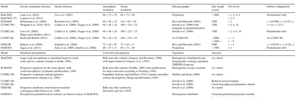
Table 1. Summary of model simulations in the ensemble adapted from Table 1 of Lunt et al. (2012). Additions detailing precipitation schemes are from Table 2 of Dai (2006). Some models have irregular grids in the atmosphere and/or ocean or have spectral atmospheres. The atmospheric and ocean resolution is given asX×Y×Z, whereXis the effective number of grid boxes in the zonal,Y in the meridional, and
Zin the vertical.e: eccentricity;o: obliquity;p: longitude of perihelion.
Model Eocene simulation reference Model reference Atmosphere Ocean Paleogeography Sim. length CO2levels Orbital configuration
resolution resolution (years)
HadCM3L Lunt et al. (2010) Cox et al. (2001) 96×73×19 96×73×20 Proprietary > 3400 ×1, 2, 4, 6 Preindustrial orbit
HadCM3L (T) Loptson et al. (2014) ×2, 4
ECHAM5 Heinemann et al. (2009) Roeckner et al. (2003) 96×48×19 142×82×40 Bice and Marotzke (2001) 2500 ×2 e=0.0300;o=23.25;p=270 CCSM3 (W) Winguth et al. (2010, 2012) Collins et al. (2006); Yeager et al. (2006) 96×48×26 100×116×25 Sewall et al. (2000) with 1500 ×4, 8, 16 e=0;o=23.5
marginal sea parameterisation
CCSM3 (H) Liu et al. (2009); Collins et al. (2006); Yeager et al. (2006) 96×48×26 100×122×25 Sewall et al. (2000) 1500 ×2, 4, 8, 16 Preindustrial orbit Huber and Caballero (2011)
CCSM3 (K) Kiehl and Shields (2013) Collins et al. (2006); Yeager et al. (2006) 96×48×26 100×116×25 As CCSM (W) > 2000 × ∼5 As CCSM (W) > 3600+ × ∼9
GISS-ER Roberts et al. (2009) Schmidt et al. (2006) 72×45×20 72×45×13 Bice and Marotzke (2001) 2000 × ∼4 e=0.0270;o=23.20,p=180 FAMOUS Sagoo et al. (2013) Jones et al. (2005), Smith et al. (2008). 48×37×11 96×73×20 Proprietary > 1500 ×2 Preindustrial orbit Model Stratiform precipitation Convective precipitation Vegetation Aerosols
HadCM3L Large-scale precipitation is calculated based on cloud Bulk mass flux scheme (Gregory and Rowntree, 1990), Homogenous shrubland (Lunt) As control water and ice contents (similar to Smith, 1990) with improvement by Gregory et al. (1997) Dynamically evolving vegetation
TRIFFID (Loptson)
ECHAM5 Prognostic equations for the water phases, bulk Bulk mass flux scheme (Tiedtke, 1989) with modifications Homogenous woody savannah As control cloud microphysics (Lohmann and Roeckner, 1996) for deep convection according to Nordeng (1994).
CCSM3 (W) Prognostic condensate and precipitation Simplified Arakawa and Schubert (1974; cumulus ensemble) Shellito and Sloan (2006) As control parameterisation (Zhang et al., 2003) scheme developed by Zhang and McFarlane (1995)
CCSM3 (H) Sewall et al. (2000) Reduced aerosol loading
CCSM3 (K) Sewall et al. (2000) Cloud microphysical parameters altered GISS-ER Prognostic stratiform cloud based on moisture Bulk mass flux scheme by Sewall et al. (2000) As control
convergence (Del Genio et al., 1996) Del Genio and Yao (1993)
FAMOUS Precipitation parameterisation schemes are based on those of HadCM3L. Homogenous shrubland Uncertain perturbed parameters include those relating to cloud microphysical properties
Despite extensive effort to understand the causes and na-ture of the Eocene super-greenhouse climate state, its hy-drology remains poorly characterised. Initial observations of globally widespread Eocene laterites and coals (Frakes, 1979; Sloan et al., 1992) and of enhanced sedimentation rates and elevated kaolinite in the clay fraction of many coastal sections (Bolle et al., 2000; Bolle and Adatte, 2001; John et al., 2012; Robert and Kennett, 1994; Nicolo et al., 2007) sug-gested that early Eocene terrestrial environments were char-acterised by globally enhanced precipitation and run-off rela-tive to today. Diverse geochemical proxies are now providing a more nuanced interpretation of how the spatial organisa-tion of the Eocene hydrological cycle differed from that of the present day. This is particularly the case for the PETM. In the Arctic, the hydrogen isotopic composition of
puta-tive leaf-wax compounds became enriched by ∼55 ‰ δD
at the PETM, thought to reflect increased export of moisture
from low latitudes (Pagani et al., 2006). Enrichment ofδD
in leaf waxes from tropical Tanzania, coincident with ele-vated concentrations of terrestrial biomarkers and sedimen-tation rates, has been interpreted as indicating a shift to a more arid climate with seasonally heavy rainfall (Handley et al., 2008, 2012). Whether these changes are typical of the low latitudes or are highly localised responses remains to be determined. Elsewhere, conflicting evidence for regional hy-drological changes exists: an increased PETM offset in the magnitude of the carbon isotope excursion (CIE) between marine and terrestrially derived carbonates, including from Wyoming, has been suggested to reflect increases in humid-ity and soil moisture of the order of 20–25 % (Bowen et al., 2004). Other studies utilising leaf physiognomy and pale-osols suggest that the North American continental interior became drier at the onset of the PETM or alternated between wet and dry phases (Kraus et al., 2013; Smith et al., 2007; Wing et al., 2005).
These proxies collectively indicate an early Eocene hydro-logical cycle different to that of the present day, but only limited proxy–model comparisons have been made (Pagani et al., 2006; Speelman et al., 2010; Winguth et al., 2010). Such comparisons will be valuable for a better understand-ing of the climate of warm time intervals but also offer an alternative to temperature by which to evaluate GCM per-formance and/or constrain boundary conditions. Some
anal-ysis of model precipitation and P− sensitivity to imposed
CO2(Winguth et al., 2010), paleogeography (e.g. Roberts et
al., 2009), and parametric uncertainty (Sagoo et al., 2013; Kiehl and Shields, 2013) has been undertaken, but the range of hydrological behaviour simulated within different models has not yet been assessed. Broadly, GCMs indicate that
fu-ture warmth will be associated with an exacerbatedP−E
distribution, as increased water vapour transport occurs from moisture divergence zones into convergence zones (Held and Soden, 2006; Chou and Neelin, 2004). An intensified hydro-logical cycle, associated with increased meridional transport of water vapour is therefore consistent with regions of both wetting and drying, although this thermodynamic response may be complicated by dynamical shifts in atmospheric cir-culation (e.g. Chou et al., 2009; Bony et al., 2013; Chad-wick et al., 2012). However, these hypotheses remain largely untested on ancient climate states. Lunt et al. (2012) un-dertook a model intercomparison of early Eocene warmth, EoMIP, based on an ensemble of 12 Eocene simulations undertaken in four fully coupled atmosphere–ocean climate models, a summary of which is given in Table 1. This demon-strated differences in global surface air temperature of up to
9◦C for a single imposed CO2and differing regions of CO2
-induced warming, but the implications for the hydrological cycle have not been considered.
compare to preindustrial simulations and vary between mod-els in the EoMIP ensemble? (2) How consistently do the
EoMIP GCMs simulate regional precipitation andP−E
dis-tributions? (3) Do differences between models affect the de-gree of match with existing proxy estimates for mean annual precipitation?
2 Model descriptions
The EoMIP approach of Lunt et al. (2012) is distinct from formal model intercomparison projects which utilise a com-mon experimental design (e.g. PMIP3, Paleoclimate Mod-elling Intercomparison Project Phase III, Taylor et al., 2012; CMIP5, Coupled Model Intercomparison Project, Phase 5; Braconnot et al., 2012). Instead, the EoMIP models differ in their boundary conditions and span a plausible early Eocene
CO2range, utilise different paleogeographic reconstructions,
and specify different vegetation distributions. This is in addi-tion to internal differences in model structure and physics, including precipitation-relevant parameterisations such as those relating to convection and cloud microstructure. Whilst this may hinder the identification of reasons for inter-model differences, the ensemble spans more fully the uncertainty in boundary conditions, which is appropriate for deep-time climates such as the early Eocene.
The ensemble, summarised in Table 1, includes a range of published simulations of the early Eocene carried out with fully dynamic atmosphere–ocean GCMs. We extend the EoMIP ensemble as originally described by Lunt et al. (2012) to include simulations published by Sagoo et al. (2013), Kiehl and Shields (2013), and Loptson et al. (2014). A brief description of each model and the corresponding simulation is given below. Each model produces large-scale (stratiform) and convective precipitation separately, also summarised in
Table 1. Greenhouse gases other than CO2are only varied
in some of the simulations and are held at preindustrial lev-els in a number of the modlev-els; we have therefore estimated
the forcing in terms of net CO2 equivalent, as detailed
be-low. We refer to the simulations throughout this paper in
terms of their atmospheric CO2level relative to preindustrial
conditions (i.e. an Eocene simulation with an atmospheric
CO2 concentration twice that of preindustrial conditions is
referred to as “x2” and one with a concentration four times that value is referred to as “x4”).
2.1 HadCM3L
HadCM3L (Hadley Centre Coupled Model, Version 3L) is a version of the GCM developed by the UK Met Office (Cox et al., 2000). Eocene simulations performed at x2, x4, and x6
preindustrial concentrations of atmospheric CO2 were
pre-sented by Lunt et al. (2010) in their study of the role of ocean circulation as a possible PETM trigger via methane hydrate destabilisation. In these simulations, models were integrated for more than 3400 years to allow intermediate-depth ocean
temperatures to equilibrate. Both the atmosphere and ocean
are discretised on a 3.75◦longitude×2.5◦latitude grid, with
19 vertical levels in the atmosphere and 20 in the ocean. Veg-etation is set to a fixed globally homogenous shrubland.
The effect of using an interactive vegetation model, TRIFFID (Top–down Representation of Interactive Foliage and Flora Including Dynamics; Cox, 2001), on tempera-ture proxy–model anomalies was considered by Loptson et al. (2014), who performed simulations at x2 and x4
preindus-trial CO2, continuations of those of Lunt et al. (2010). Within
each grid cell, TRIFFID simulates the fractional coverage of five plant functional types, which in turn influences climate via feedbacks including albedo, evapotranspiration rate, and carbon cycling (Cox et al., 2001). This study indicated that
for a given prescribed CO2, the inclusion of dynamic
vegeta-tion acts to warm global climate via albedo and water vapour feedbacks. We refer to these simulations as HadCM3L (T). The effect of dynamic vegetation on precipitation distribu-tions and global precipitation rate was additionally briefly considered, but comparisons to precipitation proxy data or to other models have not been undertaken.
2.2 FAMOUS
FAMOUS (Fast Met Office/UK Universities Simulator) is an alternative version of the UK Met Office’s GCM, adopt-ing the same climate parameterisations as HadCM3L but solved at a reduced spatial and temporal resolution in the atmosphere (Jones et al., 2005; Smith et al., 2008).
Atmo-spheric resolution is 7.5◦longitude×5◦latitude, with 11
lev-els in the vertical, whilst the ocean resolution matches that of HadCM3L. Both modules operate at an hourly time step. Be-cause of its reduced resolution, FAMOUS has been used for transient simulations with long run times and in perturbed pa-rameter ensembles where a large number of simulations are required (Smith and Gregory, 2012; Williams et al., 2013). Sagoo et al. (2013) used FAMOUS to study the effect of parametric uncertainty on early Eocene temperature distribu-tions by varying 10 climatic parameters which are typically poorly constrained in climate models. Their results demon-strated that a globally warm climate with a reduced Equator-to-pole temperature gradient can be achieved at x2
preindus-trial CO2level. Of the 17 successful simulations which ran
2.3 CCSM3
We utilise three sets of simulations performed with CCSM3 (Community Climate System Model, Version 3), a GCM developed by the US National Centre for Atmospheric Research in collaboration with the university community (Collins et al., 2006). The first set was initially used by Liu et al. (2009) in their study of Eocene–Oligocene sea sur-face temperatures and subsequently compared to terrestrial proxy data in a study of the early Eocene climate equability problem by Huber and Caballero (2011). These simulations
are configured with atmospheric CO2at x2, x4, x8, and x16
preindustrial. Models were integrated for between 2000 and 5000 years until the sea surface temperature was in
equilib-rium. The atmosphere is resolved on a 3.75◦ longitude by
∼3.75◦latitude (T31) grid with 26 levels in the vertical, and
the ocean is resolved on an irregularly spaced dipole grid. The prescribed land surface cover follows the reconstructed vegetation distribution utilised in Sewall et al. (2000). Fol-lowing the approach of Lunt et al. (2012), we refer to these simulations as CCSM3 (H).
The second set of simulations, which we refer to as CCSM3 (W), was described by Winguth et al. (2010) and Shellito et al. (2009) and conducted at x4, x8, and x16
preindustrial CO2. Relative to the CCSM3 (H) simulations,
these simulations utilised a solar constant reduced by 0.44 %, adopted an updated vegetation distribution (Shellito and Sloan, 2006), and utilised a marginal sea parameterisation, resulting in paleogeographic differences, particularly in po-lar regions. However, the major difference between the simu-lations is that the CCSM3 (W) simusimu-lations utilise a modern-day aerosol distribution, whereas CCSM3 (H) adopts a re-duced loading for the early Eocene based on a hypothesised lower early Eocene ocean productivity (Kump and Pollard, 2008; Winguth et al., 2012).
The third set of simulations, CCSM3 (K), is described in Kiehl and Shields (2013). This study investigated the sen-sitivity of Eocene climatology to the parameterisation of aerosol and cloud effects, specifically by altering cloud mi-crophysical parameters including cloud drop number and ef-fective cloud drop radii. Modern-day values from pristine re-gions are applied homogenously across land and ocean. Sim-ulations were performed at two greenhouse gas concentra-tions corresponding to possible pre- and trans-PETM atmo-spheric compositions which are equivalent to about x5 and
about x9 preindustrial CO2levels respectively.
Paleogeogra-phy and vegetation distribution are the same as those used in CCSM3 (W), and the solar constant is reduced by 0.487 % relative to the preindustrial value. Changes in precipitation
distribution between high- and low-CO2 simulations have
previously been shown for the CCSM3 (W) and CCSM3 (K) simulations (Winguth et al., 2010; Kiehl and Shields, 2013), but how robust these Eocene distributions are to GCM choice remains unknown.
2.4 ECHAM5/MPI-OM
The ECHAM5/MPI-OM (European Centre Hamburg Model, Version 5, and Max Planck Institute Ocean Model) model is the GCM of the Max Planck Institute for Meteorology (Roeckner et al., 2003), used by Heinemann et al. (2009) in their study of reasons for early Eocene warmth. The
simu-lation was performed at x2 preindustrial CO2, using the
pa-leogeography of Bice and Marotzke (2001) and a globally homogenous vegetation cover, with lower albedo but larger leaf area and forest fraction than preindustrial, equivalent to a modern-day woody savannah. Atmosphere components are
resolved on a Gaussian grid, with a spacing of 3.75◦
longi-tude and approximately 3.75◦latitude. Relative to the
prein-dustrial simulation, methane is increased from 65 to 80 ppb and nitrous oxide from 270 to 288 ppb for the Eocene, but these are negligible relative to change in radiative forcing
as-sociated with a doubling of preindustrial CO2. Latitudinal
precipitation distributions in the simulation relative to the preindustrial conditions were considered by Heinemann et al. (2009) and elevated convective precipitation at high lati-tudes was suggested to be consistent with convective clouds as a high-latitude warming mechanism (Abbot and Tziper-man, 2008).
2.5 GISS-ER
The E-R version of the Goddard Institute for Space Stud-ies model (GISS-ER; Schmidt et al., 2006) was utilised by Roberts et al. (2009) in their study of the impact of Arctic pa-leogeography on high-latitude early Eocene sea surface tem-perature and salinity. Here, we include the simulation with the open Arctic paleogeography of Bice and Marotzke (2001) which is also utilised in the ECHAM5 simulation. The
simu-lation was performed with CO2at x4 preindustrial levels and
CH4 at x7 preindustrial levels, equivalent to a total Eocene
greenhouse gas forcing of about x4.3 preindustrial CO2. The
atmospheric component of GISS-ER has a grid resolution of
4◦latitude by 5◦longitude with 20 levels in the vertical; the
ocean model is of the same horizontal resolution but with 13 levels. Vegetation is prescribed as in Sewall et al. (2000). The hydrological cycle is shown to be intensified for the Paleo-gene simulation, with elevated global precipitation and evap-oration rates, but spatial precipitation distributions were not studied.
3 Results
3.1 Preindustrial simulations
Figure 1.Preindustrial precipitation distributions as simulated in the EoMIP models (modern paleogeography). Panels (a, b, d, f, h, j), and
(l) show mean annual precipitation (MAP; left colour bar), and panels (c, e, g, i, k), and (m) show anomalies relative to CMAP observations
(1979–2010) calculated as model minus observations (right colour bar). The inset to the right of (a) indicates the principal features of the CMAP precipitation distribution, as discussed in the text.
precipitation, in addition to temperature distributions, differ between the GCMs in the ensemble (Table 1). We initially summarise model skill in simulating preindustrial mean an-nual precipitation (MAP) to provide context for our Eocene model intercomparison and to identify which, if any, precipi-tation structures are unique to the Eocene and which are more fundamentally related to errors particular to a given GCM.
Figure 1 shows preindustrial MAP distributions for each GCM in the EoMIP ensemble and anomalies for each prein-dustrial simulation relative to CMAP observations (Centre for Climate Prediction, Merged Analysis of Precipitation), which incorporates both satellite and gauge data (Yin et al.,
2004; Gruber et al., 2000). The following observations can be made.
x1 x2 x4 x8 x16 800
900 1000 1100 1200 1300 1400 1500
CO2 x preindustrial
Global mean precipitation, mm/year
(b)
10 15 20 25 30 35
800 900 1000 1100 1200 1300 1400 1500
Global mean surface air temperature /°C
Global mean precipitation, mm/year
(c)
10 15 20 25 30 35
800 900 1000 1100 1200 1300 1400 1500
Global mean surface air temperature /°C
(d)
x1 x2 x4 x8 x16
10 15 20 25 30
CO x preindustrial2
Global mean surface air temperature, °C
(a)
CCSM3(W) CCSM3(K) GISS-ER ECHAM
Preindustrial FAMOUS HadCM3L
CCSM3(H)
HadCM3L + TRIFFID
Global mean precipitation, mm/year
Figure 2.Global sensitivity of the Eocene hydrological cycle in the EoMIP simulations. Global mean surface air temperature relative to model CO2(a), global mean precipitation rate relative to model
CO2(b), and global mean surface air temperature (c); note the
log-arithmic scale on the horizontal axis in (a, b). Preindustrial sim-ulations and Eocene simsim-ulations are shown as circles and squares respectively. The CCSM3 simulations share a preindustrial simula-tion, shown in red. Open circle symbols in (b) show modern-day estimates of global precipitation rate calculated based on CMAP data (red), GPCP data (Global Precipitation Climatology Project; Adler et al. 2003; blue), and Legates and Willmott (1990) climatol-ogy (green). Also shown is the sensitivity of the hydrological cycle to global mean surface air temperature in the 17 successful simu-lations of Sagoo et al. (2013) using FAMOUS (d; diamonds), with HadCM3L simulations (blue; Lunt et al., 2010) shown for compar-ison. All best-fit lines are based on Eocene simulations only.
ECHAM5, and CCSM3 all simulate the ITCZ mean an-nual location north of the Equator, but the South Pa-cific Convergence Zone (SPCZ) generally extends too far east within the Pacific and is too zonal, with precip-itation equalling that to the north of the Equator to pro-duce a “double-ITCZ” – a common bias in GCMs (Dai, 2006; Lin et al., 2007; Brown et al., 2011). The localised rain belt minimum is a result of the Pacific cold tongue, not present in GISS-ER, which instead simulates a sin-gle convergence zone with high mean annual precipita-tion across the tropics. Other biases which appear com-mon across the ensemble include too little precipitation over the Amazon (Yin et al., 2013; Joetzjer et al., 2013), over-precipitation in the Southern Ocean (Randall et al., 2007, and references therein), and biases in the position
of rainfall maxima in the Indo-Pacific (e.g. Liu et al., 2014).
ii. Errors over the continents are smaller than those over the oceans. Absolute errors in MAP are largest over the high-precipitation tropical and subtropical oceans and
frequently exceed 150 cm yr−1in the case of ITCZ and
SPCZ offsets. Over the continents, anomalies are
gener-ally no greater than 60 cm yr−1, and more than 80 % of
the multimodel mean terrestrial surface has an anomaly
less than 30 cm yr−1. In low-precipitation regions, these
errors still result in significant percentage errors (Fig. S1 in the Supplement).
iii. Models show regional differences in precipitation skill. Figure 1 demonstrates that some precipitation biases are individual to particular GCMs. Whilst these are most noticeable over the high-precipitation tropical and sub-tropical oceans, such as offsets in the location of maxi-mum precipitation intensity or strength of storm tracks, relative differences within low-precipitation continental regions can also be considerable (Mehran et al., 2014; Phillips and Gleckler, 2006). This is particularly the case for the Sahel region of northern Africa and the Antarctic continental interior (Fig. S2). We hypothesise that GCMs applied to the study of paleoclimates are also likely to show significant regional differences in their precipitation distribution, underlining the importance of model intercomparison. Given that all of the models simulate the principal features of MAP distribution, we carry all forward to our Eocene analysis. However, it is important to recognise that significant model biases in simulating precipitation distribution exist, even where boundary conditions are well constrained.
3.2 Sensitivity of the global Eocene hydrological cycle to greenhouse gas forcing
The EoMIP model simulations were configured with a range
of plausible early Eocene and PETM atmospheric CO2
lev-els, yielding a range of global mean surface air tempera-tures (Lunt et al., 2012). It is therefore possible to evalu-ate how consistently precipitation revalu-ates are simulevalu-ated across
the GCMs (i) for a given CO2level, (ii) for a given global
mean temperature or, in the case of those models for which multiple simulations have been performed, (iii) for a given
CO2 change, and (iv) for a given global mean temperature
change. Closure of the GCM global hydrological budget requires that total annual precipitation and evaporation are equal, providing there is no net change in water storage; the imbalances, summarised in Table S1 in the Supplement are
< 0.01 mm day−1 equivalent. The mean annual global
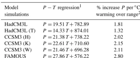
Table 2.Summary of relationships between global surface air tem-perature and precipitation rate.1T: SAT (◦C);P: global precipi-tation (mm yr−1).2Precipitation sensitivity is calculated over the range of 15–30◦C.
Model P−T regression1 % increasePper◦C simulations warming over range2
HadCM3L P=19.51T+782.89 1.81 HadCM3L (T) P=14.33T+874.01 1.32 CCSM3 (H) P=21.38T+738.22 2.02 CCSM3 (K) P=22.61T+710.60 2.15 CCSM3 (W) P=21.46T+696.28 2.11 FAMOUS P=27.86T+576.22 2.80
derived from preindustrial simulations (filled circles) are in relatively good agreement with observational data, providing confidence in this measure.
All of the EoMIP models exhibit a more active hydro-logical cycle for the Eocene (Fig. 2b; squares) compared to that simulated in the corresponding preindustrial simulations
(Fig. 2b; circles). For a given CO2, the models vary in the
intensity of the hydrological cycle they simulate; for exam-ple, ECHAM5 has a global precipitation rate at x2
preindus-trial CO2 comparable to that of CCSM3 (W) at about x12
CO2. In the remainder of this section, we discuss reasons for
these differences, which can be attributed to (i) differences
in Eocene boundary conditions, including CO2, (ii) variation
of poorly constrained parameter values, and (iii) more funda-mental differences in the ways in which the models simulate hydrology.
The GCMs within the EoMIP ensemble differ in their
global mean temperature for a given CO2(e.g. Lunt et al.,
2012; Fig. 2a). Consequently, the global precipitation rate for each ensemble member is shown in Fig. 2c relative to its globally averaged surface air temperature. This demonstrates that much of the variation between models in precipitation rate arises from these temperature differences. For
exam-ple, the elevated precipitation rate in the x2 CO2ECHAM5
is explained by this model’s warmth, being globally > 5◦C
warmer than HadCM3L at the same CO2. Similarly, the
en-hanced precipitation rate in the CCSM3 (K) simulations at
both about 5 times CO2 and about 9 times CO2 relative
to those simulated in CCSM3 (H) and CCSM3 (W) are at-tributable to warmer surface temperatures in CCSM3 (K), re-sulting from alterations to cloud condensation nuclei (CNN) parameters, with a reduction in low-level cloud acting to in-crease short-wave heating at the surface (Kiehl and Shields, 2013). The reduced aerosol loading in CCSM3 (H) results in surface warming relative to CCSM3 (W) (Fig. 2a), which explains much of the 7–8 % increase in strength of the
hydro-logical cycle across the CO2range studied. There are effects
beyond those induced by surface temperature, however. For example, for a given surface air temperature, the global pre-cipitation rate is consistently weaker in CCSM (W) relative
to CCSM (H) (Fig. 2c), possibly a result of modified aerosol– cloud interactions due to the changes in prescribed aerosols in CCSM (H).
The degree to which the global hydrological cycle will in-tensify with future global warming has received much atten-tion (e.g. Allen and Ingram, 2002; Held and Soden, 2006;
Trenberth, 2011). Held and Soden (2006) show a∼2%
in-crease in global precipitation per degree of warming for AR4 GCMs forced with the A1B emissions scenario but with no-table inter-model variability. For those simulations with
mul-tiple CO2forcing, it is possible to estimate how this
sensitiv-ity varies for the Eocene. We show the dP /dTrelationships
for each model as well as the increase in percentage of
pre-cipitation for a 1◦C temperature increase over the range of
15–30◦C (Table 2). Both CCSM3 and HadCM3L appear to
be broadly comparable at∼1.8–2.1% increase in the
inten-sity of the hydrological cycle for each degree of warming, consistent with the future-climate simulations.
Some variation in the intensity of the hydrological cycle simulated by the EoMIP models may be expected to oc-cur independently of global mean surface air temperature. For preindustrial conditions, boundary conditions are largely constant across the simulations (atmospheric composition, continental positions, orography, and ice sheet distribution),
yet the simulations show a spread of ∼0.30 mm day−1,
which exceeds the precipitation increase for a doubling of
CO2from x2 to x4 preindustrial levels in both CCSM3 (H)
(0.13 mm day−1) and HadCM3L (0.18 mm day−1).
Differ-ences in global precipitation rate between the preindustrial simulations are not explained by differences in temperature (Fig. 2b) but may relate to more fundamental differences in model physics, particularly between HadCM3L and CCSM3 (W) given that a more active hydrological cycle is consis-tently simulated in HadCM3L for both the Eocene and prein-dustrial conditions. Further simulations using equivalent pre-cipitation parameterisation schemes for large-scale and con-vective precipitation would be required to fully evaluate this hypothesis.
For both x2 and x4 CO2 simulations, the HadCM3L
simulations that include the TRIFFID dynamic vegetation model have a near-identical precipitation rate to those
with-out (Fig. 2b). However, the x4 CO2simulation with dynamic
vegetation is substantially warmer than the x4 CO2
simu-lation with fixed homogenous shrubland. The inclusion of the dynamic vegetation model acts to warm the surface cli-mate as described in Loptson et al. (2014), but this does not yield an associated increase in precipitation. Relative to the fixed shrubland simulations, the TRIFFID simulations show a reduction in continental evapotranspiration in response to a
doubling of CO2, which results in diminished moisture
avail-ability over the tropical landmass, for a given temperature (Fig. S3). The TRIFFID simulations therefore exhibit a
re-duced hydrological sensitivity of an only∼1.3 % increase in
precipitation per degree of warming (dP /dT) compared with
In the FAMOUS simulations undertaken by Sagoo et
al. (2013; Fig. 2d), all simulations are performed at x2 CO2,
but global temperatures range between 12.3 and 31.8◦C on
account of simultaneous variation of 10 uncertain parameter values, some of which directly influence cloud formation and precipitation. Within these simulations there is also a linear relationship between surface air temperature and global
pre-cipitation (R2=0.965; n=17), suggesting that the global
intensity of the hydrological cycle remains primarily cou-pled to global temperature, despite greater scatter around the
dP /dT relationship. Despite this, the overall dP /dT
rela-tionship in FAMOUS is higher than that of HadCM3L and
HadCM3L (T), with a∼2.8 % increase in precipitation for
each degree of warming (Table 2).
In HadCM3L, the Eocene simulation at x1 CO2and
prein-dustrial simulations have similar global precipitation rates (Fig. 2a), implying that Eocene boundary conditions other
than CO2do not exert a major influence on the intensity of
the hydrological cycle, raising the global precipitation rate by
only ∼0.10 mm day−1. Moreover, even this small increase
is consistent with and likely driven by a small increase in global surface air temperature. Furthermore, the preindus-trial simulations for both CCSM3 and HadCM3L lie on, or
close to, the Eocene-derived dP /dT lines (Fig. 2c),
suggest-ing that globally, the precipitation rate for a given temper-ature is not increased or decreased for the Eocene, despite differences in low-latitude land–sea distribution, ocean gate-ways, and a lack of Eocene ice sheets. Intriguingly,
extrap-olating the dP /dCO2relationship backwards to x1 CO2for
CCSM (W) would require an Eocene precipitation rate∼7 %
above that of the preindustrial rate. This suggests a more substantial effect of Eocene boundary conditions on elevat-ing absolute precipitation rates for CCSM3 (W) than that seen in HadCM3L, but one that is still operating via tem-perature effects. GISS-ER has a marginally more vigorous hydrological cycle than the other models for a given global temperature. Roberts et al. (2009) show that the global
pre-cipitation rate in a preindustrial simulation with x4 CO2in
GISS-ER is ∼4 % greater than that of preindustrial
condi-tions, whereas the Paleogene simulation has a precipitation
rate∼23 % above that of the preindustrial conditions.
There-fore, non-greenhouse gas Paleogene boundary conditions are crucial in elevating the precipitation rate in this model, in contrast to HadCM3L. However, this also appears to be me-diated by temperature effects, given that the Eocene simu-lations of Roberts et al. (2009) are also substantially warmer
than preindustrial geography simulations x4 CO2greenhouse
gas concentrations.
-50 0 50 0 500 1000 1500 2000 2500 3000 PTOT mm/year
-50 0 50 -40 -20 0 20 40 HadCM3L
TSURF °C
-50 0 50 0 500 1000 1500 2000 2500 3000 PCV mm/year
-50 0 50 0 200 400 600 800 1000 1200 PLS mm/year
-50 0 50 0 500 1000 1500 2000 2500 3000
-50 0 50 -40 -20 0 20 40 FAMOUS
-50 0 50 0 500 1000 1500 2000 2500 3000
-50 0 50 0 200 400 600 800 1000 1200 -50 0 50 0 500 1000 1500 2000 2500 3000
-50 0 50 -40
-20 0 20 40
CCSM3H and CCSM3K
-50 0 50 0 500 1000 1500 2000 2500 3000
-50 0 50 0 200 400 600 800 1000 1200
x1 x2 x4 x6
E1 E4 E7 E10 E13 E16 E17
x2 x4 x8 x16 x5 x9
HadCM3L
CCSM3_H CCSM3_K
FAMOUS
x2 ECHAM5
Preindustrial (HadCM3L, CCSM3, FAMOUS) Preindustrial (ECHAM5)
latitude, °N latitude, °N latitude, °N
(b) (c) (a) (e) (f) (d) (h) (i) (g) (k) (l) (j)
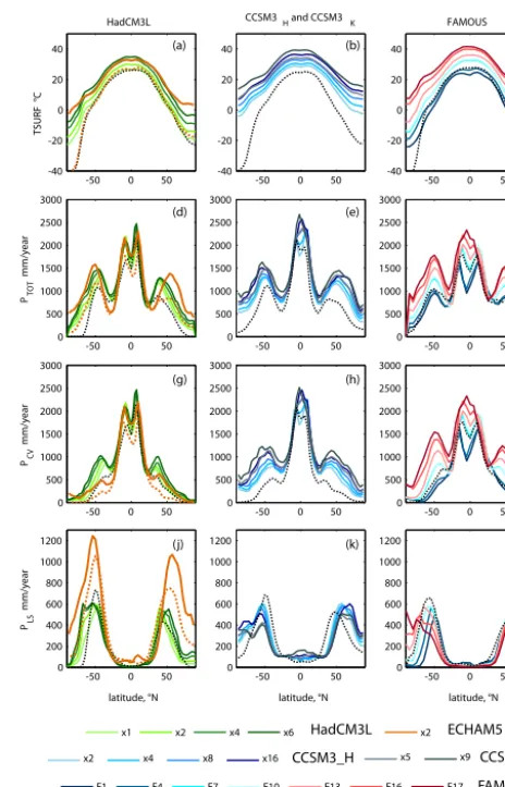
Figure 4.Latitudinal temperature and precipitation distributions in the HadCM3L and ECHAM5 (left), CCSM3 (H) and CCSM3 (K) (centre), and FAMOUS (right) members of the EoMIP ensemble. Panels (a–c) show mean surface air temperature, (d–f) total pre-cipitation rate, (g–i) convective prepre-cipitation, and (j–l) large-scale precipitation. The HadCM3L, ECHAM5, and CCSM3 atmospheric CO2levels are shown in the key. All FAMOUS simulations are x2 CO2but differ in value for 10 uncertain parameters (Sect. 2).
Simu-lation names E1–E17 shown in the legend correspond to those given by Sagoo et al. (2013). Black dotted lines show output from prein-dustrial simulations, with the exception of ECHAM5, shown in or-ange.
3.3 Variability in mean annual precipitation (MAP) distribution
3.3.1 Spatial distribution of MAP
to preindustrial simulations, the Eocene distributions ex-hibit increased precipitation at high latitudes as a conse-quence of elevated temperatures in these regions. In CCSM in particular, the Eocene is characterised by a more glob-ally equable precipitation rate: the expansion of zones of highest precipitation in the Eocene relative to preindus-trial conditions is muted compared with a more exten-sive loss of low-precipitation regions. Additional support for this is provided by a comparison of mean precipitation rates for land and ocean (Table S2). The preindustrial ra-tio of land : ocean precipitara-tion is maintained in the Eocene HadCM3L and ECHAM5 simulations, whereas in CCSM, precipitation rates over land and ocean are typically equal. The effects of differences in simulated surface air tempera-tures between models within the ensemble are also evident: for a given global surface temperature, HadCM3L maintains cooler poles than CCSM3 and ECHAM5 (Sect. 3.3.2), and
regions with MAP < 300 cm yr−1 persist in the Arctic and
Antarctic, even x4 CO2.
Modelled Eocene MAP features are frequently traceable to those identified in preindustrial simulations (Sect. 3.1), in-cluding the single tropical convergence zone in the
GISS-ER simulation at x4 CO2 and the double ITCZ in a
num-ber of the models. Elsewhere, the Eocene precipitation dis-tributions diverge from those of the preindustrial simulations and may be related to specific Eocene paleogeography,
el-evated CO2, or other boundary conditions. In HadCM3L,
there is a clear trend towards a more south-easterly
trend-ing SPCZ in the higher-CO2simulations, which is not
repli-cated in the warm simulations of the sister model FAMOUS. The SPCZ in CCSM3 is also far weaker in the Eocene sim-ulations, compared to preindustrial simulations. The mech-anisms which control the SPCZ in the modern day, partic-ularly its northwest–southeast orientation, are only partially understood, with zonal SST gradients, the intensity of trade winds, and the height of the Andes all suggested to be im-portant influences (Matthews, 2012; Cai et al., 2012). In the EoMIP simulations, CCSM3 shows much slacker sur-face winds at the Equator with reduced low-level conver-gence, whilst HadCM3L maintains stronger convergence of south-easterly trade winds with north-easterlies originating from the Pacific subtropical high (Fig. S4). Despite similar preindustrial precipitation distributions over tropical Africa, CCSM3 and HadCM3L strongly diverge in the Eocene, with CCSM3 showing far more intense equatorial precipitation. In CCSM3, evaporation is consistently less than the precipi-tation rate, which likely results in the recharge of soil mois-ture throughout the year and an availability of moismois-ture for convective precipitation. The FAMOUS simulations E16 and E17 represent two realisations of very warm climates with a reduced Equator–pole temperature gradient; in these sim-ulations significant increases in midlatitude precipitation are particularly accentuated over the Pacific Ocean. Increases in convection in the subtropics and midlatitudes are sufficient
-50 0 50 -500
0 500 1000 1500 2000 2500 3000 3500
Latitude °N
MAP, mm/year
-50 0 50 -1500
-1000 -500 0 500 1000 1500 2000
Latitude °N
P-E , mm/year
Eocene multimodel mean Preindustrial multimodel mean
(b) (a)
Figure 5.Multimodel mean annual precipitation (a) and mean an-nual precipitation–evaporation (P−E) rate (b) for Eocene (red) and preindustrial (blue) boundary conditions. For the Eocene mul-timodel mean, simulations have a global mean precipitation rate of 3.40±0.02 mm day−1 (Table S1); these are HadCM3L (x4), HadCM3L (T) (x4), ECHAM5 (x2), CCSM3 (H) (x4), and a lin-early interpolated distribution between the x4 and x8 CO2CCSM3
(W) simulations. Error bars represent the range in values across sim-ulations.
to eliminate the precipitation minima seen in other models at these latitudes.
For a given CO2, differing boundary conditions,
param-eterisation schemes, and simulated model air temperatures prevent direct assessment of whether Eocene regional pre-cipitation distributions are robust across different GCMss. Model simulations have a substantially different amount of water vapour in the atmosphere and differing global precip-itation rates and it is not meaningful to average these sim-ulations. Instead, we show a multimodel mean in Fig. 5 for simulations with a common global precipitation rate to pro-vide an assessment of regional variability between model simulations with the same global strength hydrological cy-cle. Elevated high-latitude precipitation for the early Eocene relative to preindustrial conditions is robust between GCMs, although absolute values remain variable between models, particularly in the Southern Hemisphere, likely due to differ-ing Antarctic orography. Differences between models in the midlatitudes are smaller, resulting in some confidence that the secondary precipitation maxima were polewards of their preindustrial location during the Eocene. Equatorial precipi-tation remains highly variable between models but is accen-tuated relative to preindustrial conditions.
3.3.2 Controls on precipitation distribution
Precipitation rates for each simulation are summarised in Table S2, including separate rates calculated over land and ocean surfaces and rates deconvolved into those arising from convective and large-scale contributions. These data show
that elevated precipitation rates in the high-CO2Eocene
al-though in the ECHAM5 model a greater percentage of pre-cipitation is generated by large-scale mechanisms in both the Eocene and preindustrial simulation. Figure 4 shows how convective and large-scale precipitation rates vary with lat-itude for a selection of the EoMIP simulations. This reveals differences between models in the mechanisms responsible for precipitation distributions which can be related to sur-face air temperature distributions. In the HadCM3L simula-tions, the midlatitude maxima in both large-scale and
convec-tive precipitation advance polewards with increasing CO2,
with precipitation increases over the high northern latitudes driven almost exclusively by enhanced large-scale precipita-tion. CCSM3 has substantially warmer poles, which results in much enhanced high-latitude large-scale precipitation rel-ative to HadCM3L, although large-scale latitudinal contribu-tions differ somewhat for preindustrial simulacontribu-tions at both low and high latitudes. In CCSM3 (K), the warmest CCSM3 simulations, polar temperatures are elevated compared to CCSM3 (H) as is total precipitation in these regions, but in this case large-scale precipitation is reduced over much of the high latitudes and the higher total precipitation is due to con-vective processes. Midlatitude precipitation maxima within the ECHAM5 simulation arise from large-scale mechanisms rather than convection; however, this is also true of the prein-dustrial simulation and does not relate to Eocene boundary conditions.
In the warmest FAMOUS simulations of Sagoo et al. (2013), the high latitudes experience particularly signifi-cant increases in large-scale precipitation, such that the max-imum values are those at the poles in the E17 simulation, and in the Southern Hemisphere the local midlatitude precipita-tion maximum is lost. Elevated midlatitude temperatures in the warm FAMOUS simulations additionally result in signif-icant increases in convective precipitation which are not sim-ulated in the cooler simulations and models. Overall, convec-tive precipitation in FAMOUS increases as both global tem-peratures rise and equatorial-to-polar temperature gradients decrease, regardless of the underlying parameter configura-tion; this emphasises the fundamental control of temperature distribution on precipitation, as opposed to the effect of al-teration of any one specific parameter.
Improvements in the simulation of precipitation in modern-day climate simulations are often related to better resolved topography (e.g. Gent et al., 2010). However, given the variety of differences in boundary conditions between the EoMIP simulations, topography appears to only have lim-ited power in explaining differences between regional pre-cipitation responses. Figure S5 shows differences in topog-raphy and precipitation rate between three sets of simula-tions with similar global precipitation rates: (i) HadCM3L and FAMOUS, where the models have similar parameterisa-tion schemes but differ in atmospheric grid resoluparameterisa-tion; (ii) CCSM3 (W) and HadCM3L – different models, but with a similar resolution; (iii) CCSM3 (W) and CCSM3 (H) – the same model but slightly different topographic
bound-Anomaly mm/year
Figure 6
-1500 -900 -300 300 900 1500
(b)
(a)
Figure 6.Anomaly plots for mean annual precipitation in millime-tres per year between high and low CO2. Eocene model simulations
for (a) HadCM3L at x6 CO2–x2 CO2and (b) CCSM3 (W) at x16–
x4 CO2.
ary conditions. The HadCM3L and CCSM3 (W) simula-tions show some substantial differences in the topography around the Rockies, with the increased elevation in CCSM3 possibly accounting for the increased precipitation in this region. However, differences in topography over the Asian subcontinent do not result in any systematic differences in precipitation rate. Regions of similar topography elsewhere, including over the tropics, have far more divergent precipi-tation responses between the models, which do not relate to local differences in topography.
For HadCM3L and CCSM3, simulations at different CO2
concentrations provide an insight into how regional Eocene precipitation distributions are impacted by warming, and
anomaly plots for high CO2 simulations minus low CO2
simulations are shown in Fig. 6. For the same CO2
Figure 7. Percentage of mean annual precipitation falling in the extended summer season (MJJAS for Northern Hemisphere, NDJFM for Southern Hemisphere; early Eocene paleogeography); regions with > 55 % summer precipitation are outlined in blue. Results from preindustrial simulations are shown in the Supplement. CO2for each model simulation is shown above each plot. The FAMOUS simulations
are both at x2 CO2.
2012), but the anomalies for x16–x4 CO2(CCSM (W)) and
x6–x2 CO2 (HadCM3L) display similar global changes in
temperature and therefore precipitation rate on account of
similar dP /dT relationships (Fig. 2; Table 2). Intriguingly,
HadCM3L displays far greater spatial contrasts in net precip-itation change, particularly over the ocean: between the pair of HadCM3L simulations, some 23 % of the Earth’s surface experiences an increase or decrease in precipitation greater
than 60 cm yr−1, compared to just 6 % in the CCSM3
sim-ulations. Ignoring differences in the spatial pattern of atmo-spheric circulation, such as those relating to differing SPCZ
Peri-Table 3.Percentage of land surface characterised by extended sum-mer precipitation > 55 % MAP by model and by fractionation CO2
increase from preindustrial (PI) conditions.
Model PI ×1 ×2 ×4/5 ×6/8/9 ×16
CO2 CO2 CO2 CO2 CO2
HadCM3L 60.1 66.3 62.6 57.7 52.3
HadCM3L (T) 62.0 51.6
ECHAM5 50.1 41.6
GISS-ER 47.7 37.6
CCSM3 (H) 50.1 47.3 44.2 42.4 35.1
CCSM3 (K) 47.5 34.1
FAMOUS 48.9 28.1 E16
23.6 E17
Tethys and along the coastline of equatorial Africa. There-fore, although models within the EoMIP ensemble exhibit similarities in their global rate of precipitation change with respect to temperature, regional precipitation distributions are strongly model dependent.
3.4 Precipitation seasonality
The evolution and timing of the onset of global monsoon sys-tems in the Eocene has been the subject of debate (Licht et al., 2014; Sun and Wang, 2005; Wang et al., 2013). Proxy studies for the early Eocene have highlighted differences in precipitation seasonality relative to modern conditions (Greenwood et al., 2010; Greenwood, 1996; Schubert et al., 2012) and geochemical and sedimentological changes at the PETM have also been attributed to changes in seasonal-ity (Sluijs et al., 2011; Schmitz and Pujalte, 2007; Hand-ley et al., 2012). Previous modelling work utilising CCSM3 has suggested that much of the mid–late Eocene was mon-soonal, with up to 70 % of annual rainfall occurring dur-ing one extended season in northern and southern Africa, North and South America, Australia, and Indo-Asia (Huber and Goldner, 2012). However, GCMs have been shown to differ greatly in their prediction of future monsoon systems (e.g. Turner and Slingo, 2009; Chen and Bordoni, 2014), and therefore we examine the similarities and differences in Eocene models with respect to the seasonality of their pre-cipitation distributions.
Figure 7 shows the percentage of precipitation falling in the extended summer season (MJJAS for Northern Hemi-sphere; NDJFM for Southern Hemisphere) following the approach of Zhang and Wang (2008) also utilised in the Eocene studies of Huber and Goldner (2012) and Licht et al. (2014). This metric has been shown to correlate well with the modern-day distribution of monsoon systems. Overall, the models show a global distribution of early Eocene
mon-soons in high-CO2 climates that is similar to those
simu-lated under preindustrial simulations (Fig. S7). Australia is markedly less monsoonal than in preindustrial simulations due to its more southerly Eocene paleolocation. Note that re-gions where winter season precipitation dominates fall at the
lower end of the scale, these tend to be over the ocean surface but also include regions around the Peri-Tethys and both the Pacific and Atlantic US coasts.
HadCM3L is notable in that it is more seasonal at high latitudes, simulating an early Eocene monsoon centred over modern-day Wilkes Land region of Antarctica. Although proxy data have suggested highly seasonal precipitation regimes for both the Arctic (Schubert et al., 2012) and Antarctic (Jacques et al., 2014) during this interval, these
sys-tems are maximised in the x2 CO2simulation and weaken
somewhat in the simulations with elevated CO2. This arises
due to the high-temperature seasonality of Arctic and Antarc-tic Eocene regions in HadCM3L relative to the other mod-els (e.g. Gasson et al., 2014). In austral winter, Antarctic temperatures are sufficiently low to suppress precipitation,
whilst this constraint is lifted somewhat in the higher-CO2
simulations, which produce more equable rainfall distribu-tion. Crucially, the effect of elevated global warmth on the extent of Eocene monsoons is consistent across the models,
with higher-CO2simulations associated with a decline in
ter-restrial areas with seasonal precipitation regimes (Table 3). HadCM3L simulates a 6 % reduction in the extent of terres-trial regions influenced by monsoonal regimes for the Eocene
(HadCM3L×1 CO2) relative to the preindustrial simulation;
this reduction appears to be related to the warmer surface temperatures and the absence of the Antarctic ice sheet.
3.5 P−E distributions
The difference between precipitation and evaporation (P−
E) is essential for understanding the wider impacts of an
en-hanced Eocene hydrological cycle. Over land, this parameter broadly determines how much precipitation will become soil water and surface run-off, the partitioning itself being de-pendent on the land surface and vegetation schemes within the models (e.g. Cox et al., 1998; Oleson et al., 2004). Over
the ocean,P−Edrives differences in salinity which can
af-fect the Eocene ocean circulation (Bice and Marotzke, 2001;
Waddell and Moore, 2008). We show mean annual (P−E)
budgets for each of the EoMIP simulations in Fig. 8. In
warmer climates, an exacerbation of existing (P−E) is
ex-pected – that is, the wet become wetter and the dry drier, as the moisture fluxes associated with existing atmospheric circulations intensify (Held and Soden, 2006). Broadly, the EoMIP simulations support this paradigm for the Eocene relative to preindustrial conditions (Fig. 5). CCSM3 shows fairly minor changes in the boundaries between net
precipi-tation and net evaporation zones at higher CO2(Fig. 8),
al-though the net evaporation zones in HadCM3L do migrate polewards over the eastern Pacific and North Atlantic at high
CO2. Other dynamic changes within HadCM3L are coupled
-1000 -500 0 500 1000
E-P, mm/year
-50 0 50
-4 -2 0 2 4
flux, PW
(b)
-50 0 50 -50 0 50 -50 0 50
latitude, °N
(c)
(a) (d)
(f) (g)
(e) (h)
x1 x2 x4 x6
E16 E17
x2 x4 x8 x16
x4 x2
HadCM3L CCSM3_H
ECHAM5
FAMOUS GISS-ER ECMWF E - P
Preindustrial (HadCM3L, CCSM3, FAMOUS, ECHAM5) Preindustrial (GISS-ER)
Figure 9. Latitudinal E−P distributions (top) and implied northwards latent heat flux (bottom) in the EoMIP simulations. The black lines indicate preindustrial simulations, with dotted and unbroken lines in (d, h) corresponding to the GISS-ER and ECHAM5 simulations respectively. Heat flux expressed in petawatts (1 PW=1015 W). ObservationalE−P in (a) is based on European Centre for Medium-range Weather Forecasts (ECMWF) European Reanalysis (ERA) data (Dee et al., 2011).
(P −E) balance in this region. Over continents the models
also display different responses ofP−Eto warming. For
ex-ample, over equatorial and northern Africa, HadCM3L
simu-lates increasingly wet climates in the high-CO2simulations,
driven by increases in precipitation coupled to reductions in evaporation. In CCSM3, the net moisture balance is less re-sponsive with respect to temperature, although intense equa-torial precipitation means this region is much wetter than in HadCM3L.
Because of the large latent heat fluxes involved in evapo-ration and condensation, the global hydrological cycle acts as a meridional transport of energy. Net evaporation in the subtropics stores energy in the atmosphere as latent heat, re-leasing it at high latitudes via precipitation (Pierrehumbert, 2002). An intensified hydrological cycle, associated with in-creased atmospheric transport of water vapour, has there-fore been suggested as a potential mechanism for reducing the Equator–pole temperature gradient during greenhouse climates (Ufnar et al., 2004; Caballero and Langen, 2005).
By integrating the area-weighted estimates of P−E with
latitude, we show how these contributions differ between the EoMIP models and associated preindustrial simulations (Fig. 9). Relative to preindustrial climatology, the intensi-fication of the hydrological cycle associated with increased drying in the net evaporative zones and increased moistening of the net precipitation zones implies a stronger latent heat flux. Within the EoMIP ensemble, the implied high poleward energy fluxes of the E16 and E17 FAMOUS simulations
and x2 CO2 ECHAM5 simulation are particularly
signifi-cant. GISS-ER has a particularly strong low-latitude
equato-rially directed latent heat transfer which arises from the much elevated Eocene precipitation rate in the deep tropics. The asymmetry in some of the models’ implied flux is due to a hemispheric imbalance in precipitation and evaporation. For example, in the FAMOUS E17 simulation, there is greater precipitation than evaporation in the Southern Hemisphere, and so more energy is released from the atmosphere by latent heat than is stored, meaning that the implied heat flux does not cross 0 at the Equator. However, since total precipitation is equal to total evaporation globally (Table S1), this is bal-anced out in the Northern Hemisphere; note that the intense evaporation zone over the North Atlantic is not matched in the Southern Hemisphere for this model. In the majority of
the other models, there is greater symmetry inP−E with
latitude and the implied flux crosses close to the origin of the graph on Fig. 9.
At face value, it may seem that the elevated latent heat transport at mid- to high latitudes could contribute towards the reduced Equator–pole temperature gradient in the EoMIP simulations, but we note that theoretical and modelling-based studies suggest that increased latent heat transport is asso-ciated with an increased Equator–pole temperature gradient (Pagani et al., 2013). Within the EoMIP ensemble, merid-ional temperature gradients and global surface air temper-atures covary, and so it is not possible to separate clearly the effects of these different controls (Fig. S8). Neverthe-less, these results illustrate that relative to preindustrial con-ditions, the Eocene hydrological cycle acts to elevate the meridional transport of latent heat, particularly around 45–
50◦N and S of the Equator.
4 Proxy–model comparison
0 500 1000 1500 2000 2500
(a) Axel Heiberg Island. Paleocoordinates ~75°N 45°W, late Lutetian. M ea n an nu al pr ec ip ita tio n m m /y r
(b) Northwest Territories. Paleocoordinates ~65°N 94°W, Paleocene.
0 1000 2000
3000 (d) Central Europe. Paleocoordinates ~47°N 7°W, Lutetian. (e) ODP Site 913. Paleocoordinates ~66°N 8°W, 49 - 48 Ma. (f) Antarctica Wilkes Land. Paleocoordinates ~75°S 120°E,
53.6 - 51.9 Ma.
0 1000 2000
3000 (g) Western US Interior. Paleocoordinates 50°N 95°W. (h) Waipara, New Zealand. Paleocoordinates ~55°S 160°W,
early Eocene.
(i) Mahenge, Tanzania.
0 1000 2000 3000 4000 5000
(j) Laguna del Hunco, Argentina. Paleocoordinates ~47°S 67°E, EECO.
(k) Chickaloon Fm, Alaska. Paleocoordinates ~70°N 120°W, Paleocene-Eocene.
(l) Antarctic Peninsula.
0 2000 4000
(m) Cerrejon Fm, Colombia. Paleocoordinates ~2°N 57°W, c.58 Ma.
(c) SE Australia. Paleocoordinates ~60°S 160°E, early Eocene.
Paleocoordinates ~67°S 52°W, early-mid Eocene. Paleocoordinates ~12°S 20°E, 46 Ma.
2 4 6 2 4 2 2 2 4 2 4 8 16 4 8 16 5 9 2 4 6 2 4 2 2 2 4 2 4 8 16 4 8 16 5 9 2 4 6 2 4 2 2 2 4 2 4 8 16 4 8 16 5 9
2 4 6 2 4 2 2 2 4 2 4 8 16 4 8 16 5 9 2 4 6 2 4 2 2 2 4 2 4 8 16 4 8 16 5 9
2 4 6 2 4 2 2 2 4 2 4 8 16 4 8 16 5 9
2 4 6 2 4 2 2 2 4 2 4 8 16 4 8 16 5 9
2 4 6 2 4 2 2 2 4 2 4 8 16 4 8 16 5 9 2 4 6 2 4 2 2 2 4 2 4 8 16 4 8 16 5 9 2 4 6 2 4 2 2 2 4 2 4 8 16 4 8 16 5 9
2 4 6 2 4 2 2 2 4 2 4 8 16 4 8 16 5 9 2 4 6 2 4 2 2 2 4 2 4 8 16 4 8 16 5 9
2 4 6 2 4 2 2 2 4 2 4 8 16 4 8 16 5 9
HadCM3L HadCM3L + TRIFFID
FAMOUS ECHAM5 GISS-ER
CCSM3_H CCSM3_W CCSM3_K
Geologic estimate Bed C Bed B Bed A - E Ark
rose
BC 51.6 CA 51.6 BC 51.3 CA 51.3 BC 55.5 CA 55.5
Bass Basin Site 1172 Gippsland Hotham Heigh
ts
D
ean
’s M
arsh - ear
ly/mid E oc ene Br andy C reek
CA PT CA PT >90 CA TE CA TE
>90
BC PT BC PT >90 BC TE BC TE
>90 A ll C al 1 A ll C al 2 L7 C al 1 L7 C al 2
Cal 1 Cal 2
LH13 LH2 LH 4 LH6
Bear P
aw
Sepulcher Kisinger Wind R
vr Clar kf or kian Big M ulti La tham Sour dough N
ilandLittle M US188 NLR US188 LAA
Dragon Glacier, 49 - 44 Ma
Fossil Hill James Ross early Eocene LAA BC CA LAA WP BC BC WP
Seagull R iv er M ackenzie R iv er Seagull R iv er M ackenzie R iv er G
eiseltal Messel F
m
Cer
rejon
ODP 913
49 - 51 Ma early
Eocene late Paleocene
Figure 10.Proxy–model comparisons for mean annual precipitation (MAP) for the EoMIP ensemble: (a) Axel Heiberg Island, data from Greenwood et al. (2010); (b) Northwest Territories, data from Greenwood et al. (2010); (c) southeastern Australia and Tasmania, data from Greenwood et al. (2005) and Contreras et al. (2014); (d) central Europe, data from Mosbrugger et al. (2005) and Grein et al. (2011); (e) Ocean Drilling Program (ODP) Site 913, data from Eldrett et al. (2009); (f) Wilkes Land, data from Pross et al. (2012); (g) western US interior, data from Wilf et al. (1998) and Wilf (2000); (h) Waipara, New Zealand, data from Pancost et al. (2013); (i) Mahenge, Tanzania, data from Jacobs and Herendeen (2004) and Kaiser et al. (2006); (j) Argentina, data from Wilf et al. (2005); (k) Chickaloon Formation, Alaska, data from Sunderlin et al. (2011, 2014); (l) Antarctic Peninsula, data from Hunt and Poole (2003) and Poole et al. (2005); (m) Cerrejon Formation, data from Wing et al. (2009). Error bars show the mean with range based on nine model grid cells closest to given paleocoordinates. Full details are given in the Supplement, Table S3.
Paleoprecipitation estimates are primarily produced by two distinct paleobotanic methods: leaf physiognomy and NLR approaches. In the former, empirical univariate and multivariate relationships have been established between the size and shape of modern angiosperm leaves and the cli-mate in which they grow, with smaller leaves predominat-ing in low-precipitation climates (e.g. Wolfe, 1993; Wilf et al., 1998; Royer et al., 2005). The NLR approach estimates paleoclimate by assuming that fossilised specimens have the
ap--20 0 20 -2000
-1000 0 1000 2000
∆T data-model, SAT °C
∆
P data-model, MAP mm/year
HadCM3L
-20 0 20
-2000 -1000 0 1000 2000
∆T data-model, SAT °C
∆
P data-model, MAP mm/year
FAMOUS E17
-20 0 20
-2000 -1000 0 1000 2000
∆T data-model, SAT °C
∆
P data-model, MAP mm/year
CCSM3 HUBER
-20 0 20
-2000 -1000 0 1000 2000
∆T data-model, SAT °C
∆
P data-model, MAP mm/year
CCSM3 KIEHL
(b) (a)
(d) (c)
Figure 11.Surface air temperature and mean annual precipitation proxy–model anomalies for low- and high-CO2climates shown by
closed and open circles respectively. Simulations are at x2 and x6 the CO2levels for HadCM3L (a), E17 for FAMOUS (b), x2 and x16 the CO2for CCSM3 (H) (c), and x5 and x9 CO2for CCSM3
(K) (d). The data points represent averaged signals for the sites shown in Fig. 10. Estimates of maximum (minimum) error are cal-culated as anomalies between the highest (lowest) data estimate and the lowest (highest) value within the local model grid.
proaches, competing influence of other climatic variables on leaf form (Royer et al., 2007).
Our data compilation is provided in Table S3. Some of the data has been compared previously with precipitation rates from an atmosphere-only simulation performed with isoCAM3 (isotope-enabled Community Atmosphere Model,
version 3) for the Azolla interval (∼49 Ma; Speelman et al.,
2010). Our proxy–model comparison includes data for the remainder of the early–mid-Eocene, including a number of recently published estimates such that the geographic spread is widened to include estimates from Antarctica (Pross et al., 2012), Australia (Contreras et al., 2013; Greenwood et al., 2003), New Zealand (Pancost et al., 2013), South America (Wilf et al., 2005), and Europe (Eldrett et al., 2014; Mos-brugger et al., 2005; Grein et al., 2011). We select Ypresian-aged data where multiple Eocene precipitation rates exist, in-cluding estimates for the PETM (Pancost et al., 2013), but additionally include some Lutetian and Paleocene data, par-ticularly in regions where Ypresian data do not exist. This approach is justified in some respects given the range of
plau-sible Eocene CO2 with which simulations have been
per-formed. However, each data point is an independent estimate of precipitation for a given point in time, and direct
com-Longitude, °E
Latitude, °N
0 50 100 150 200 250 300 350
-80 -60 -40 -20 0 20 40 60 80
Existing paleobotanic Eocene precipitation estimates Regions where multimodel coeffiecient of variation >40% Regions where multimodel standard deviation > 360 mm/year
Figure 12.Summary of regions which show a significant model spread, based on the Eocene multimodel mean described in Fig. 5. Paleobotanical estimates of quantitative precipitation rate included in the data compilation are shown by green markers. Regions where the standard deviation is greater than 1 mm day−1 (i.e. 360 mm yr−1) are marked by a red outline and regions where the coefficient of variation (standard deviation / multimodel mean) is greater than 40 % are outlined blue.
parisons between data points are hindered given that consid-erable climatic change occurred throughout this interval (e.g. Zachos et al., 2008; Littler et al., 2014); comparisons are par-ticularly difficult at sites where age control is poor and the proxies could potentially reflect a range of climatic states or
atmospheric CO2(Sect. 1).
Figure 10 shows paleobotanical estimates for MAP for a range of the data in Table S3, along with model-estimated rates for each of the EoMIP simulations. Mean precipitation estimates from each model are derived by averaging over grid boxes centred on the paleolocation in a similar approach to Speelman et al. (2010). This is a nine-cell grid of three by three grid boxes for HadCM3L, GISS-ER, ECHAM5, and CCSM3, although in some instances an eight-cell grid of two by four is used along paleocoastlines. Differing model resolutions and land–sea masks result in averaging signals from slightly different paleogeographic areas, but this ap-proach allows for an assessment of the regional signal, and error bars are included to show the range of precipitation rates present within the locally defined grid. In the reduced-resolution model, FAMOUS, mean and range are derived from two by two grid boxes to ensure that regional clima-tologies remain comparable. Error bars on the geologic data are generally provided as described in the original publica-tions, with further details also provided in Table S3.