www.earth-surf-dynam.net/1/29/2013/ doi:10.5194/esurf-1-29-2013
©Author(s) 2013. CC Attribution 3.0 License.
Earth
Surface
Dynamics
The role of hydrological transience in
peatland pattern formation
P. J. Morris1, A. J. Baird2, and L. R. Belyea3
1Soil Research Centre, Department of Geography and Environmental Science, University of Reading,
Reading, RG6 6DW, UK
2School of Geography, University of Leeds, Leeds, LS2 9JT, UK
3School of Geography, Queen Mary University of London, 327 Mile End Road, London, E1 4NS, UK
Correspondence to: P. J. Morris (p.j.morris@reading.ac.uk, paul.john.morris@gmail.com)
Received: 7 May 2013 – Published in Earth Surf. Dynam. Discuss.: 6 June 2013 Revised: 18 September 2013 – Accepted: 30 September 2013 – Published: 16 October 2013
Abstract. The sloping flanks of peatlands are commonly patterned with non-random, contour-parallel stripes of distinct micro-habitats such as hummocks, lawns and hollows. Patterning seems to be governed by feedbacks among peatland hydrological processes, plant micro-succession, plant litter production and peat decomposi-tion. An improved understanding of peatland patterning may provide important insights into broader aspects of the long-term development of peatlands and their likely response to future climate change.
We recreated a cellular simulation model from the literature, as well as three subtle variants of the model, to explore the controls on peatland patterning. Our models each consist of three submodels, which simulate: peatland water tables in a gridded landscape, micro-habitat dynamics in response to water-table depths, and changes in peat hydraulic properties.
We found that the strength and nature of simulated patterning was highly dependent on the degree to which water tables had reached a steady state in response to hydrological inputs. Contrary to previous studies, we found that under a true steady state the models predict largely unpatterned landscapes that cycle rapidly be-tween contrasting dry and wet states, dominated by hummocks and hollows, respectively. Realistic patterning only developed when simulated water tables were still transient.
Literal interpretation of the degree of hydrological transience required for patterning suggests that the model should be discarded; however, the transient water tables appear to have inadvertently replicated an ecolog-ical memory effect that may be important to peatland patterning. Recently buried peat layers may remain hydrologically active despite no longer reflecting current vegetation patterns, thereby highlighting the poten-tial importance of three-dimensional structural complexity in peatlands to understanding the two-dimensional surface-patterning phenomenon.
The models were highly sensitive to the assumed values of peat hydraulic properties, which we take to in-dicate that the models are missing an important negative feedback between peat decomposition and changes in peat hydraulic properties. Understanding peatland patterning likely requires the unification of cellular land-scape models such as ours with cohort-based models of long-term peatland development.
1 Introduction
1.1 Background
The surface of northern peatlands often comprises a patch-work of distinct, small-scale (<10 m; known as scale-level 1, or SL1 – Baird et al., 2009) micro-habitats, each with a
structures at horizontal scales of tens to hundreds of metres (SL2), often forming landscapes composed of strongly direc-tional, non-random patterns that may be linear and contour parallel, polygonal, or maze like (e.g. Aber et al., 2002; Ep-pinga et al., 2008; Korpela et al., 2009). Baird et al. (2009) demonstrated that the frequency distribution of water-table depths from across a peatland landscape depends not just on the proportion of the landscape covered by different micro-habitats but also on the pattern. In consequence, pat-tern may play an important role in determining peatland– atmosphere fluxes of greenhouse carbon gases (carbon diox-ide and methane), which vary with water-table depth (Bubier et al., 1993, 1995; Roulet et al., 2007). Additionally, it seems likely that the development and maintenance of peatland pat-terning is governed by the same mechanisms that control peat accumulation, decomposition, and the development of soil hydraulic properties (Belyea and Clymo, 2001; Nungesser, 2003; Eppinga et al., 2009). An improved understanding of the mechanisms that control patterning may therefore reveal fundamental rules that govern broader aspects of peatland ecosystem and soil development at the landscape scale.
Observational (e.g. Foster and Fritz, 1987; Belyea and Clymo, 2001; Comas et al., 2005) and modelling (e.g. Nungesser, 2003; Swanson, 2007) studies have identified a variety of aspatial or one-dimensional (vertical only) feed-back mechanisms that may help to explain directionless clumping of SL1 units into larger features. However, un-derstanding the highly directional nature of patterning seen in many peatlands clearly requires an explicit considera-tion of spatial interacconsidera-tions. This problem lends itself natu-rally to investigation using 2- or 3-dimensional simulation models, in which directional transfers of water, energy and nutrients, and their effects on pattern, can be explored di-rectly. Interplay between long- and short-range processes is a recurring theme in many apparently successful models of patterned landscapes, including peatlands (Rietkerk et al., 2004a, b; Eppinga et al., 2009) and other landscape types such as marshes (van de Koppel and Crain, 2006) and dry-lands (Lefever and Lejeune, 1997).
One current hypothesis on peatland pattern formation, the ponding mechanism, has been explored using cellular land-scape models in a number of previous studies. The ponding mechanism consists of a pair of competing feedbacks be-tween water-table depth, peatland micro-habitat succession, and peat hydraulic properties. Areas with deeper water tables are assumed to be more likely to support hummock vegeta-tion, whereas areas with shallower water tables are assumed to be more likely to support hollow vegetation (cf. Rydin and Jeglum, 2006). Furthermore, hummock vegetation is as-sumed to produce near-surface peat that is less permeable than that produced in hollows (cf. Ivanov, 1981). Contrast-ing micro-habitat states (hummock, hollow) between adja-cent SL1 units allow a positive feedback that reinforces local differences in water tables. Ponding occurs upslope of hum-mocks, leading to hollows there; while areas downslope of
Figure 1.Aerial photograph showing contour-parallel, striped
pat-terning on a peatland complex in the James Bay lowlands, Ontario, Canada. The directions of slope and regional water flow are from the top right to the bottom left of the picture. Horizontal distance between tops of successive ridges is approximately 5 to 10 m. Image belongs to Brian Branfireun, reproduced here with kind permission.
Table 1.Glossary of algebraic terms, including default values where appropriate, for each of the four model versions.
Symbol Description Dimensions Units Model 1 Model 2 Model 3 Model 4
B peatland surface height above arbitrary datum L m 0.22 to 4.20 m 0.22 to 4.20 m 0.48 to 4.17 m 0.48 to 4.17 m
∆te hydrological submodel runtime (steady-state criterion) T h 50 50 50 17 520 (2 yr)
d thickness of flow L m – auxiliary variable auxiliary variable auxiliary variable
H water-table height above arbitrary datum L m auxiliary variable auxiliary variable auxiliary variable auxiliary variable
K hydraulic conductivity L T−1 m s−1 – – – –
Kave depth-averaged hydraulic conductivity L T−1 m s−1 – – – –
Kdeep hydraulic conductivity of deep peat L T−1 m s−1 – 0 1.25×10⁻⁵ 1.25×10⁻⁵
Khol hydraulic conductivity of hollow peat L T−1 m s−1 – 1.0×10⁻³ 1.0×10⁻³ 1.0×10⁻³
Khum hydraulic conductivity of hummock peat L T−1 m s−1 – 5.0×10⁻⁵ 5.0×10⁻⁵ 5.0×10⁻⁵
p probability of hummock formation – – Eq. (3); Fig. 3 Eq. (3); Fig. 3 Eq. (3); Fig. 3 Eq. (3); Fig. 3
Q hummock turnover rate – – state variable state variable state variable state variable
R relative variance of hummocks per row – – state variable state variable state variable state variable
S proportion of model landscape occupied by hummocks – – state variable state variable state variable state variable
θ peat drainable porosity – – 0.3 0.3 0.3 0.3
T peat transmissivity L2T−1 m2s−1 – – – –
Thol transmissivity of hollow cells L2T−1 m2s−1 2.0×10⁻⁴ – – –
Thum transmissivity of hummock cells L2T−1 m2s−1 1.0×10⁻⁵ – – –
U net rainfall rate (precip. minus evapotran.) L T−1 mm yr−1 0 0 400 (constant) 400 (time series)
x spatial index (across-slope direction) L m – – – –
y spatial index (along-slope direction) L m – – – –
Z water-table depth below peat surface L m auxiliary variable auxiliary variable auxiliary variable auxiliary variable
Zfinal final water-table depth at end of developmental step L m state variable state variable state variable –
Zmean mean water-table depth during second half of dev. step L m – – – state variable
1.2 Aim and objectives
We recreated the SGCJ version of the ponding model to ex-plore three characteristics that we suspected may have indi-vidually or collectively led to a Type-1 error in the SGCJ studies (i.e. causing a model to predict patterning despite the ponding mechanism being incapable of generating patterning in reality):
i. Numerical implementation of shallow groundwater flow: the transmissivity, T [dimensions of L2T−1] (see Table 1 for a glossary of algebraic terms), of any grid square in the original SGCJ models depends entirely on whether that square is currently a hummock or a hol-low. Only two values of T are possible, one canonical value for hummocks, Thum, and one for hollows, Thol. A
more realistic scheme would have been to assign canon-ical values of a more intrinsic property of peat such as saturated hydraulic conductivity, Khumand Khol[L T−1],
to hummocks and hollows, respectively, and to calcu-late transmissivity as the product of K and the thickness of flow in that square, thereby allowing for continuous variation in T across the model landscape. We extended the hydrological submodel from the SGCJ models in this way in order to remove any unrealistic constraints that the simplified numerical implementation of shallow groundwater flow may have placed upon overall model behaviour. We also wished to explore the effects of the absolute values of T or K (as appropriate) upon model behaviour.
ii. Conceptual hydrogeological setting: the original SGCJ models considered only a shallow layer of near-surface peat, and assumed that deeper peat was impermeable to groundwater flow. The top few decimetres of peat
are usually the most permeable (e.g. Fraser et al., 2001; Clymo, 2004) and are therefore prone to the most rapid subsurface flow, although deeper peat is rarely truly im-permeable. Indeed, a number of studies have indicated that drainage through deep peat layers may play an im-portant role in peatland development and the ability of these ecosystems to self-organise (e.g. Ingram, 1982; Belyea and Baird, 2006; Morris et al., 2011). The as-sumption of impermeable peat below the uppermost few decimetres may have prevented the SGCJ models from representing a potentially important hydrological inter-action between surficial hydraulic structures and deeper peat layers. Furthermore, in the original SGCJ models rainfall was not included; the only inputs of water to the models were from shallow groundwater flow and/or surface runon. In order to address these conceptual is-sues we experimented with the effects of incorporating a permeable lower layer and driving the model using simulated rainfall.
iii. Dependence on hydrological transience: the original SGCJ authors reported that strong striped patterning oc-curred in their models under “steady-state” hydrolog-ical conditions, whereby micro-habitat transitions only took place once the simulated water-table map had equi-librated with with the current distribution of hummocks and hollows (and so the spatial arrangement of transmis-sivity) (see Sect. 2 for full model description). The cri-terion used to determine steady state considers the pro-portion of cells in which the rate of water-table change [L T−1] is less than a threshold rate. Steady-state
(not reported here in full) with our own version of the ponding model indicated that the simulations reported in the earlier SGCJ studies may not have attained true hydrological steady state and that, curiously, pattern-ing only developed under intermediate steady-state cri-teria where water tables were still transient. We chose to experiment with the effects of hydrological tran-sience upon model patterning, either by manipulating the water-table steady-state criterion, or by driving the model with a real time series of rainfall data.
2 Models and methods
2.1 Overview
We began with a model that was as similar as possible to that employed by Couwenberg (2005), as far as the origi-nal model description allows. As well as this replica model (henceforth, Model 1) we created three additional models (Models 2, 3 and 4) with slightly altered routines. We de-signed Model 2 so as to address the numerical implementa-tion issue identified in objective (i), while we designed Mod-els 3 and 4 so as to address the conceptual issues identified in objective (ii) (see Sect. 1.2, above; and Table 2). Each of the four models may be thought to consist of three submod-els that simulate: shallow saturated groundwater movements and the spatial distribution of water-table depths at SL1 (hy-drological submodel); switches in micro-habitat type (eco-logical submodel); and changes in peat soil hydraulic prop-erties (soil propprop-erties submodel). Model time progresses in developmental steps: during each developmental step the hy-drological submodel is run until a predetermined steady-state criterion is met. The output from the hydrological submodel is a map of water-table depths within the model landscape. The ecological submodel then simulates a new micro-habitat map within the model landscape on the basis of the water-table map, such that every cell in the model landscape is assigned one of two binary micro-habitat types: hummock or hollow. Finally, the soil properties submodel uses the new micro-habitat map to reassign the spatial distribution of near-surface peat hydraulic properties. The new map of peat hy-draulic properties is then used as an input to the hydrological model at the beginning of the next developmental step. As with the SGCJ studies, our models do not simulate explic-itly the processes of peat formation or decomposition, and therefore do not incorporate a peat mass balance. Rather, the models represent plant community succession as a shifting mosaic of SL1 tiles superimposed onto a static peat land-form.
2.2 Hydrological submodel
The hydrological submodel uses a modification of the Di-giBog model of peatland saturated hydrology (Baird et al., 2012). We took the original DigiBog Fortran 95 code and
added routines to represent the ecological and hydrophys-ical submodels. In the current study we deactivated Digi-Bog’s peat accumulation, decomposition and hydrophysical subroutines described by Morris et al. (2012). We refer the reader to Baird et al. (2012) for a comprehensive descrip-tion of DigiBog’s governing equadescrip-tions and numerical imple-mentation, although a few points are pertinent here. DigiBog represents a peatland as a grid of vertical peat columns; in plan each column is equivalent to one square grid cell in the SGCJ models, although DigiBog also allows for ver-tical variation in peat hydraulic properties. Horizontal sat-urated groundwater flow occurs between adjacent columns (four-square neighbourhood) at a rate equal to the product of the harmonic mean of inter-cell transmissivity (the prod-uct of depth-averaged hydraulic condprod-uctivity and the thick-ness of flow) and inter-cell hydraulic gradient, according to the Boussinesq equation (see also McWhorter and Sunada, 1977):
∂H ∂t =
∂ ∂x
Kave(d)
θ d ∂H
∂x
!
+∂∂ y
Kave(d)
θ d ∂H
∂y
!
+Uθ, (1)
where H is water-table height [L] above an arbitrary datum; t is simulated time [T]; x and y are across-slope and along-slope horizontal spatial dimensions, respectively [L]; Kaveis
depth-averaged hydraulic conductivity [L T−1];θis drainable porosity of the peat [dimensionless], assumed constant at 0.3; d is thickness of flow [L], defined as the height of the water table, H, minus the height of the impermeable base layer; and U is net rainfall [L T−1]. Because U is added directly to the saturated zone it may be thought of as a black-box representation of total precipitation minus the sum of sur-face runoff, interception, evapotranspiration and unsaturated water-storage change.
The hydrological model is run for a predetermined length of simulated time in order to allow the water-table map to change in response to the boundary conditions and the cur-rent distribution of hydraulic properties. In Models 1 to 3, the length of time that the hydrological model is allowed to run, ∆te[T], before an ecological transition takes place (Sect. 2.3)
determines how close to a genuine steady state the simulated water tables are. Short equilibration times lead to highly tran-sient water tables that are still changing rapidly and are far from being in equilibrium with the hydrological inputs or boundary conditions; the opposite is true of long runtimes. In Models 1, 2 and 3 we varied∆tebetween 1 h (highly transient
water tables) and 10 000 h (approximately 417 days; highly steady water tables) to examine the effect of the steady-state criterion upon model behaviour. We performed only a single simulation with Model 4, with∆te=17 520 h (equal to two
years of simulated time), and introduced hydrological tran-sience by driving the model using a daily rainfall time series derived from observed data (Sect. 2.5).
We performed a simple test on Models 1, 2 and 3 in order to verify that increasing∆te led to increasing hydrological
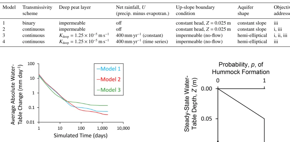
Table 2.Summary of the four models and the objectives addressed by each.
Model Transmissivity Deep peat layer Net rainfall, U Up-slope boundary Aquifer Objectives
scheme (precip. minus evapotran.) condition shape addressed
1 binary impermeable off constant head, Z=0.025 m constant slope iii
2 continuous impermeable off constant head, Z=0.025 m constant slope i, iii
3 continuous Kdeep=1.25×10⁻⁵m s−1 400 mm yr−1(constant) impermeable (no-flow) hemi-elliptical i, ii, iii
4 continuous Kdeep=1.25×10⁻⁵m s−1 400 mm yr−1(time series) impermeable (no-flow) hemi-elliptical iii
Figure 2.Time series of daily-average absolute water-table change
per grid square during five-year test periods with Models 1, 2 and 3. See main text for full details. Note the logarithmic scales on both axes.
developmental steps with all default parameter values (see Table 1) and∆te=50 h. We then allowed the hydrological
submodel to continue for a further five years of simulated time, without any further changes in the spatial distributions of micro-habitats or peat properties. For each simulated day of the five-year test we calculated the daily sum of absolute water-table movements in each model grid square, and then averaged these absolute changes for all grid squares. In all three models the average rate of water-table change declined rapidly from initial values of between 14 and 19 mm day−1
to between 0.03 and 0.14 mm day−1 by the end of the
five-year test period (Fig. 2). The tests indicate that water-table behaviour for all three models converges on steady state with increasing∆te.
The depth of the water table below the surface at any point in model time is given simply by
Z=B−H, (2)
where Z is water-table depth [L]; and B is the height of the peatland surface relative to the arbitrary datum [L]. We refer to the value of Z at the end of a developmental step as Zfinal;
and the time-averaged value of Z during the second half of a developmental step as Zmean. These two metrics are used as
inputs to the ecological submodel (Sect. 2.3).
Figure 3.Graphical representation of the linear probability
func-tion used by the ecological submodel to assign hummock and hol-low states to each model cell, based on water-table depth.
2.3 Ecological submodel
In Models 1, 2 and 3 the probability, p [dimensionless], of any model cell being designated as a hummock during a given developmental step is a linear function of water-table depth, Zfinal, at the end of the previous developmental
step. When the water table is at the surface in any cell (i.e. when Zfinal=0.00 m), p=0 (i.e. that cell is necessarily
des-ignated as a hollow for the following developmental step). The value of p increases linearly with increasing water-table depth up to Zfinal=0.05 m. When Zfinalis equal to or greater
than 0.05 m, the cell is automatically designated a hummock (i.e. p=1). The relevant equations (see also Fig. 3) are
p=0.0 for Z≤0.00 m
p=20Z for 0.00 m<Z<0.05 m
p=1.0 for Z≥0.05 m, (3)
where Z is equal to either final water-table depth at the end of a developmental step, Zfinal(Models 1, 2 and 3), or
time-averaged water-table depth during the second half of a two-year developmental step, Zmean(Model 4) (see below).
based on each grid square’s time-averaged water-table depth, Zmean[L], during the second half of the previous 2 yr
devel-opmental step. The first 365 days of each develdevel-opmental step are used to allow Model 4’s simulated water tables to adjust to the newly updated distribution of peat hydraulic proper-ties, but this adjustment period is not incorporated into Zmean.
This measure was intended to ensure that Zmean in Model
4 contains no meaningful artefact of water-table geometries from earlier developmental steps. Along with a variable rain-fall time series (see Sect. 2.5, below) the use of Zmean
pro-vided a means of introducing transience to water-table be-haviour in an arguably more realistic manner than the short equilibration times used in Models 1 to 3.
2.4 Soil properties submodel
Hummocks are assumed to produce peat that is less perme-able than that produced by hollows. DigiBog’s implemen-tation of the Boussinesq equation uses depth-averaged satu-rated hydraulic conductivity, Kave, and the thickness of flow,
d, to calculate saturated groundwater flux between adjacent columns (Eq. 1). However, the original SGCJ models simply assigned a single value of transmissivity, Thum, to hummocks
and another, higher value, Thol, to hollows. Model 1 uses the
simple treatment of canonical transmissivities as per the orig-inal SGCJ models; thus, in the case of Model 1, Eq. (1) sim-plifies to
∂H ∂t =
∂ ∂x
T θ
∂H ∂x
!
+∂∂ y
T θ
∂H ∂y
!
+Uθ. (4)
We assumed default transmissivity values of Thol=2.0×
10−4m2s−1and T
hum=1.0×10⁻⁵m2s−1, thereby preserving
the Thol to Thum ratio of 20 : 1 that led to strong
pattern-ing in the original SGCJ models. Models 2, 3 and 4 use a more sophisticated and realistic treatment allowed by Digi-Bog, whereby hummocks and hollows are assigned canonical values of hydraulic conductivity, Khumand Khol, respectively;
T for each cell is recalculated during each iteration of the hy-drological submodel as the product of K and the thickness of flow, d (height of water table above the model’s impermeable base layer) (cf. Freeze and Cherry, 1979). In this way T is able to vary in a continuous manner based on water-table po-sition, which is more realistic than the simple binary-T treat-ment of the original SGCJ models (Eq. 1). For Models 2, 3 and 4, we assumed default values of Khol=1.0×10⁻³m s−1
and Khum=5.0×10⁻⁵m s−1, thereby giving a Khol to Khum
ratio of 20 : 1. In models 1, 2 and 3 we also manipulated the default values of T or K by factors of between 0.05 and 20 in line with objective (i). In Model 1 we varied Thumbetween
5.0×10⁻⁷and 2.0×10⁻⁴m2s−1; and T
holbetween 1.0×10⁻⁵
and 4.0×10⁻³m2s−1, whilst always maintaining a T
hol to
Thumratio of 20 : 1. Similarly, in Models 2 and 3 we varied
Khumbetween 2.5×10⁻⁶ and 1.0×10⁻³m s−1; and Khol
be-tween 5×10⁻⁵and 2×10⁻²m s−1, whilst maintaining a K hol
to Khumratio of 20 : 1.
2.5 Model spatial and temporal domains; boundary conditions
We implemented all simulations in a 70 (across-slope, x di-rection) ×200 (along-slope, y direction) grid of 1 m×1 m grid squares. In Models 1 and 2, the simulated peat aquifer overlaid a sloping impermeable base (replicating the assump-tion of an impermeable lower peat layer in the SGCJ mod-els). Both the peat surface and the impermeable base had a constant slope of 1 : 50; the permeable upper peat had a uni-form thickness of 0.2 m. In Models 3 and 4 we assumed the thick, lower peat layer is also permeable with its own hy-draulic conductivity, Kdeep, meaning that K for each cell is
depth-averaged to account for the vertical transition in K be-tween the upper and lower layers. Baird et al. (2012) pro-vide a full description of DigiBog’s calculation of Kave and
inter-cell T . We used the groundwater mound equation (In-gram, 1982) to calculate the dimensions of a deep peat layer that is hemi-elliptical in cross section, has a uniform K of 1.25×10⁻⁵m s−1, is 200 m from central axis to the margin, is
underlain by a flat impermeable base, and receives a net wa-ter input (from an implied upper peat layer) of 155 mm yr−1.
The resulting deep peat layer was 3.97 m thick along its cen-tral axis, curving elliptically down to 0.28 m at the peatland’s margin. Within DigiBog, this deep layer was overlain by a surficial, more permeable layer, which, like Models 1 and 2, was 0.2 m thick.
We allowed all simulations to run for 100 developmental steps; the initial condition consisted of randomly generated water tables, between 0.0 and 0.05 m below the peat surface, in each cell. The initial micro-habitat and soil-properties maps were based on this random initial water-table map in the usual manner described above.
0 10 20 30 40 50 60 70 80
1 61 121 181 241 301 361
D
aily
Rainf
all (
m
m
da
y
-1
)
Day of Year
ObservedScaled
Figure 4.365-day time series of daily observed rainfall, and its
conversion to net rainfall, U, after scaling by a factor of 0.245. See main text for full details.
Model 3 were maintained by a constant simulated net rainfall rate of U=400 mm yr−1 (U is assumed to be net of
evapo-transpiration, interception and runoff; hence, its low value). We drove Model 4 using a daily time series of U. We took 365 days of daily rainfall data from close to Malham Tarn Moss, a raised bog in North Yorkshire, United Kingdom, for the calendar year 2011. The rain gauge recorded precipitation on 294 days of that year, with an annual total of 1633 mm of precipitation. Maximum daily precipitation for the year was 78.6 mm on 10 August. We multiplied each daily rainfall to-tal in the time series by approximately 0.245 so as to give an annual total of 400 mm of net precipitation, equal to the con-stant U assumed in Model 3, whilst maintaining a plausible temporal variation (Fig. 4). During each 2 yr developmental step in Model 4 we cycled twice through the 365-day rain-fall series. By using the same year of rainrain-fall data repeatedly in this way we were able to induce water-table transience without the potentially complicating effects of inter-annual variability in rainfall patterns. The thick peat deposit repre-sented in Models 3 and 4, and the fact that their groundwa-ter mounds were maintained by simulated net rainfall, means that they might be thought to be most representative of om-brotrophic raised bogs.
2.6 Analysis
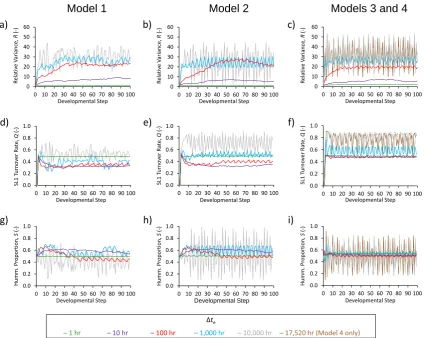
Previous studies (e.g. Andreasen et al., 2001; Eppinga et al., 2009) have demonstrated that the human eye is a pow-erful tool for assessing pattern strength in landscape mod-els, and we used a visual appraisal of the two-dimensional micro-habitat maps produced by the four models as our pri-mary means of estimating simulated pattern strength. In ad-dition we calculated the relative variance, R [dimensionless], of hummocks per across-slope row of cells, following the method of Swanson and Grigal (1988), as an objective and reproducible metric of pattern strength. The value of R
in-creases with pattern strength: values less than 2 indicate un-ordered landscapes without discernible patterning; values of R greater than 4 represent highly ordered landscapes with clear, strong patterning. We also calculated the proportion, S [dimensionless], of model cells occupied by hummocks dur-ing each developmental step. Finally, we calculated model turnover rate, Q [dimensionless], defined as the proportion of model cells that undergo a transition from hummock to hollow, or vice versa, in each developmental step.
3 Results
3.1 Hydrological transience
In Models 1, 2 and 3, the strength of across-slope, striped patterning at SL2 initially increased strongly with increas-ing hydrological steadiness, from an apparently entirely un-ordered, random mixture of hummocks and hollows at SL1 when∆te=1 h, to peak “strengths” at around∆te=100 h (for
Models 1 and 2) or 50 h (Model 3). This increase in pattern-ing strength is evident from both a visual appraisal of the final micro-habitat maps (Fig. 5), and an increase in the val-ues of relative variance, R, with increasing∆te(Fig. 6a, b, c).
For values of∆tegreater than 50 h (Models 1 and 2) and 20 h
(Model 3), an increase in the spatial scale of the simulated SL2 stripes is apparent with increasing ∆te (i.e. the stripes
became broader in the y (along-slope) direction). Increasing ∆te also led to SL2 stripes whose upslope and downslope
edges were increasingly straight and sharply defined (Fig. 5). For values of∆tegreater than 100 h (Models 1 and 2) or 50 h
(Model 3), the simulated SL2 stripes had broadened to the point of appearing to be “over-developed”, such that they no longer resembled realistic peatland striped patterning (cf. Fig. 1).
As well as governing the spatial configuration of simulated patterning, the value of∆tealso affected the temporal
dynam-ics of Models 1, 2 and 3. For low values of∆te, turnover rates
of model cells were high: when∆te=1 h, approximately half
of all cells would undergo a transition from designation as a hummock to a hollow (or vice versa) during each develop-mental step, providing further indication of a random land-scape. Increasing∆teled to a reduction in turnover rates in
Models 1 and 2 as SL2 structures began to stabilise, to a min-imum of approximately 40 % of cells per developmental step when ∆te=100 h (Fig. 6d, e). Increasing ∆te had little
ef-fect on turnover rates in Model 3 until∆te=1000 or 10 000 h
(Fig. 6f). The temporal trends in SL1 turnover rate and pro-portional hummock coverage also indicate what appears to be a limit cycle in the behaviour of all models under highly stringent hydrological steady-state criteria. Particularly when ∆te=17 520 (Model 4 only) or 10 000 h, and to a lesser
ex-tent when∆te=1000 h, the models exhibited a cyclical
Figure 5.Final micro-habitat maps after 100 developmental steps, showing effects of increasing∆te on patterning in typical simulations
with Model 1 (top panel), Model 2 (middle panel) and Model 3 (bottom panel). The value of∆teassumed for each simulation is indicated
immediately above the map. Light pixels represent hummocks, dark pixels represent hollows. Low values of y represent upslope locations (y=0 is the upslope boundary); high values of y represent downslope locations (y=200 is the downslope boundary); as such, groundwater flow is generally down the page. All maps have the same horizontal (x, y) scale as that shown for the upper-leftmost map.
a dry landscape with deeper water tables, dominated by hum-mocks; and a wet landscape with water tables near the bog surface, dominated by hollows (Fig. 6). The contrast be-tween the wet and dry states was particularly pronounced in Model 2, which cycled between approximately 15 % and 95 % hummock coverage when∆te=10 000 h (Fig. 6h). The
single simulation with Model 4 (∆te=17 520 h) behaved in
a very similar manner to Models 1, 2 and 3 when ∆te=
10 000 h, predicting nearly homogeneous, unpatterned land-scapes (Fig. 7) that cycled rapidly between being dominated by hummocks and hollows (Fig. 6f, i).
In all simulations that generated striped SL2 pattern-ing, those SL2 units migrated consistently downslope (not
shown) in the same manner as that previously reported in the published accounts of the SGCJ models.
3.2 Simplified calculation of transmissivity
0 10 20 30 40 50 60
0 10 20 30 40 50 60 70 80 90 100
R ela tiv e V aria nce, R ( -) Developmental Step 0 10 20 30 40 50 60
0 10 20 30 40 50 60 70 80 90 100
R ela tiv e V aria nce, R ( -) Developmental Step 0.0 0.2 0.4 0.6 0.8 1.0
0 10 20 30 40 50 60 70 80 90 100
Humm . Pr oportion, S ( -) Developmental Step 0.0 0.2 0.4 0.6 0.8 1.0
0 10 20 30 40 50 60 70 80 90 100
Humm . Pr oportion, S ( -) Developmental Step 0.0 0.2 0.4 0.6 0.8 1.0
0 10 20 30 40 50 60 70 80 90 100
SL1 T urn o ver Ra te, Q ( -) Developmental Step 0.0 0.2 0.4 0.6 0.8 1.0
0 10 20 30 40 50 60 70 80 90 100
SL1 T urn o ver Ra te, Q ( -) Developmental Step
a)
b)
c)
d)
e)
f)
g)
h)
i)
Model 1
Model 2
Models 3 and 4
0.0 0.2 0.4 0.6 0.8 1.0
0 10 20 30 40 50 60 70 80 90 100
Humm . Pr oportion, S ( -) Developmental Step 0.0 0.2 0.4 0.6 0.8 1.0
0 10 20 30 40 50 60 70 80 90 100
SL1 T urn o ver Ra te, Q ( -) Developmental Step 0 10 20 30 40 50 60
0 10 20 30 40 50 60 70 80 90 100
R ela tiv e V aria nce, R ( -) Developmental Step Δte
– 1 hr – 10 hr – 100 hr – 1,000 hr – 10,000 hr – 17,520 hr (Model 4 only)
Figure 6.Influence of hydrological equilibration time,∆te, over temporal development of relative variance of hummocks per model row, R
(top row); SL1 turnover rate, Q (middle row); and proportion of model landscape occupied by hummocks, S (bottom row); in Models 1 (left column), 2 (middle column), 3 and 4 (right column).
to both changing values of ∆teand changing absolute
val-ues of peat permeability. Both models developed realistic looking, contour-parallel SL2 stripes over the entire model domain for intermediate values of∆te. In both models the
striped patterning was relatively weak and discontinuous for ∆te=15 and 20 h; the patterns were stronger and continuous
when∆tewas between 35 and 100 h; the SL2 stripes became
unrealistically broad at ∆te=1000 h, and were mainly
ab-sent when∆te=10 000 h (Fig. 5). Temporal patterns of
sum-mary metrics (SL1 turnover rate, hummock proportion, rel-ative variance of hummocks per row) were qualitrel-atively and quantitatively similar between models 1 and 2, and again re-sponded similarly to changes in∆te(Fig. 6) and the ratio of
Thumto Tholor Khumto Khol(not shown).
3.3 Hydrogeological setting
Any artefacts introduced to model behaviour by the simplify-ing assumptions made in the original SGCJ models about the hydrogeological setting of the simulated peatland (see ob-jective ii, above) would have been evident as differences in
behaviour between Model 2 (impermeable deep peat layer; constant-head upslope boundary condition; zero rainfall ad-dition; constant slope of peatland surface) and Model 3 (per-meable deep peat layer; no-flow upslope boundary; con-stant net rainfall rate of 400 mm yr−1; hemi-elliptical aquifer shape). Model 2 simulations that generated patterning did so over the entire model domain, although the same was not true of Model 3. Striped patterning at SL2 developed in Model 3 only in the downslope portion of the model domain. Further-more, the area of the model domain that exhibited pattern-ing extended upslope with increaspattern-ing values of∆te. For
in-stance, when∆te=10 h, Model 3 only produced striped
pat-terning within 60 m or so of the downslope boundary, but when ∆te=100 h the patterned area covered the majority
of the model domain and extended as far as approximately 140 m from the downslope boundary (Fig. 5). Clear, con-tinuous striped patterning that extended all the way across the across-slope direction (x direction) of the model domain developed in Model 3 at much lower values of∆te than in
Figure 7.Final micro-habitat map after 100 developmental steps from Model 4, with ∆te=17 520 h (2 yr). Light pixels represent
hummocks, dark pixels represent hollows. Low values of y repre-sent upslope locations (y=0 is the upslope boundary); high val-ues of y represent downslope locations (y=200 is the downslope boundary); as such, groundwater flow is generally down the page.
although sharply defined, continuous SL2 stripes in Model 2 did not develop for values of∆teless than 35 h. Additionally,
Model 3 behaved differently from Model 2 in terms of its re-sponses to changes in the absolute values of peat hydraulic conductivity (see below).
3.4 Manipulation of peat properties
Modest changes in the absolute values of T or K brought about large changes in the nature and strength of simulated patterning in Models 1, 2 and 3, although the nature of these responses varied between models. In Models 1 and 2, the lowest values of T or K led to largely unpatterned landscapes, dominated by apparently random distributions of hummocks and hollows, with either a complete absence of patterning (×0.05 treatment) or very weak, discontinuous patterning
(×0.1 treatment) (Fig. 8). In both Models 1 and 2, pattern
strength increased with increasing values of T or K up to the default combination. For combinations of T and K greater than the default values, Models 1 and 2 both predicted an in-crease in the spatial scale of SL2 stripes in a manner similar to the effect of increasing∆te; for the×10 and×20 treatments
Model 1 became almost a uniform landscape of hummocks with only small SL2 groupings of hollows. The behaviour of Model 3 was quite different. Only the default and the×0.2
treatments generated any kind of contour-parallel stripes; all other treatments produced near-uniform, unpatterned land-scapes composed almost entirely of either hollows (for the
×0.05 and×0.1 treatments) or hummocks (for the×5,×10 and×20 treatments).
Figure 8.Final micro-habitat maps after 100 developmental steps,
showing effects of different combinations of Thumand Thol(in the
case of Model 1, top panel) or Khum and Khol (Model 2, middle
panel; Model 3, bottom panel) on pattern geometries in typical model runs. The values of T or K used in each simulation are in-dicated immediately above the maps, and are expressed as a factor of the default values. See main text for full explanation. Light pixels represent hummocks, dark pixels represent hollows. Low values of
y represent upslope locations (y=0 is the upslope boundary); high values of y represent downslope locations (y=200 is the downslope boundary); as such, groundwater flow is generally down the page. All maps have the same horizontal (x, y) scale as that shown for the upper-leftmost map.
4 Discussion
4.1 Hydrological transience and ecological memory The striking similarity between the patterns generated by our Models 1, 2 and 3 at intermediate values of ∆te and the
studies had not attained genuine steady-state hydrological conditions. The dependence of realistic patterning in our models on intermediate equilibration times can be reconciled with the currently popular theory that landscape patterning commonly arises from interplay between long- and short-range processes (e.g. Rietkerk and van de Koppel, 2008; see also Turing, 1952). The strength of the long-range neg-ative feedback (which acts to homogenise local differences in water-table position in response to distant hydrological boundary conditions) appears to increase as the hydrological equilibration time is lengthened. When equilibration times are very short each grid square’s water-table behaviour is in-fluenced only by its immediate neighbours, and long-range influences are unable to propagate across the model domain. Conversely, the longest equilibration times cause the sim-ulated water-table map to be dominated by its long-range boundary conditions, which, under steady state, eliminate much of the short-range effects of contrasting peat hydraulic properties in neighbouring SL1 and SL2 units. Without ad-ditional feedbacks such as those explored by Eppinga et al. (2009), it is only at intermediate values of ∆te that the
model strikes the balance of long- and short-range feedbacks seemingly required for patterning.
If the absolute values of∆te are taken literally then the
model predicts that realistic patterning only occurs if micro-succession at SL1 operates on unrealistically short timescales of hours to days, rather than years. Moreover, Model 4, in which we introduced water-table transience not through short equilibration times but through a daily rainfall series, did not generate patterning. This indicates clearly that it is the short equilibration times used in Models 1, 2 and 3, rather than simply non-steady water tables (which are also present in Model 4) that caused patterning in our simulations. It is per-haps initially tempting to discard the model in light of its reliance on hydrological transience.
However, an alternative and more abstract interpretation of the models’ dynamics allows one to conceptualise the length of a developmental step simply as a measure of hydro-logical steadiness under which succession takes place. With this in mind, we can think of succession as occurring over a period of years, during which the degree of hydrological steadiness is determined by∆te. Therefore,∆teis no longer
a literal time period during which plant community succes-sion occurs but merely a means of representing hydrological steadiness. For lower values of∆te, the water tables across
the models’ domains are not in full equilibrium with the cur-rent distribution of hummocks and hollows. As such, those water-table maps reflect the distribution of hummocks and hollows during not only the current developmental step but also partly the previous developmental step. It may be that the formation of peatland patterning relies on some ecologi-cal memory effect (cf. Peterson, 2002), such as the influence of recently buried peat that no longer reflects current posi-tions of hummocks and hollows but which remains hydro-logically important due to its shallow depth. Despite
Digi-Bog allowing for 3-dimensional variation in peat properties, the ponding model is in essence a 2-dimensional model inso-far as the new micro-habitat map during each developmental step supersedes the previous map entirely; the modelled sys-tem retains no memory of previous SL1 units or their associ-ated soil properties. As such, our models neglect some of the structural complexity that peatlands exhibit in three spatial dimensions (e.g. Barber, 1981). Our simulations with non-conservative hydrological steady-state criteria (particularly ∆te=50 and 100 h) implicitly contain a type of ecological
memory effect, because the influence of previous patterns of surface vegetation and shallow soil properties are expressed in the model’s hydrological behaviour; this memory effect decreases in strength with increasingly stringent hydrologi-cal steady-state criteria. Our results indicate that this mem-ory effect is important to the formation of patterning in the ponding model and should be investigated directly in future studies, perhaps via the use of cohort-based peat accumula-tion models (e.g. Frolking et al., 2010; Morris et al., 2011, 2012).
4.2 Peat hydraulic properties
Models 1, 2 and 3 were all highly sensitive to the abso-lute values of T or K, and patterning only occurred within a narrow region of parameter space. Even in the×0.05 and ×20 treatments, the values of T or K were well within re-ported ranges; the fact that these parameterisations failed to produce patterning suggests that a full suite of relevant pro-cesses and feedbacks has not been represented. Particularly in Model 3, in which model water-table levels are maintained by the simulated addition of rainfall, even modest changes in the absolute values of Khol and Khum caused simulations to
“run away” to either wet or dry end-member states. In sim-ulations with higher values of hydraulic conductivity Model 3 drained rapidly to the downslope boundary, causing wa-ter tables to fall below the transition zone and giving rise to uniformly dry simulated landscapes dominated by hum-mocks. Conversely, the simulations with lower values of hy-draulic conductivity caused Model 3 to drain so slowly that water tables rose to the surface of all columns, leading to uni-formly wet landscapes dominated by hollows. The same ef-fect was not evident in Models 1 and 2 because the constant-head condition at the upslope boundary maintained water-table levels within the transition zone. Nonetheless, manipu-lating T and K in Models 1 and 2, respectively, still resulted in landscapes devoid of realistic patterning by strengthening the long-range negative feedback relative to the short-range positive feedback.
decomposition of peat (e.g. Boelter, 1969; 1972; Grover and Baldock, 2013). Areas with deep water tables are prone to more rapid decomposition and more rapid collapse of pore spaces. The resultant reduction in hydraulic conductivity in turn causes peat to retain water more readily and causes decay rates to fall, stabilising system behaviour (see Be-lyea, 2009; and Morris et al., 2012). This concept is par-tially represented in the ponding model by lower values of T or K in hummocks (where peat spends more time under oxic conditions, and hence peat at the water table is more degraded and less permeable) than in hollows (where peat has a shorter residence time under oxic conditions, produc-ing better-preserved and more permeable peat at the depth of the water table). However, in the ponding model only two K values are possible, Khum and Khol, meaning that hydraulic
conductivity cannot vary as a continuous function of decom-position; the ponding model’s representation of this relation-ship may therefore be overly constrained. Modelling studies by Morris et al. (2011) and Swindles et al. (2012) have in-dicated that a continuous relationship between peat decom-position and hydraulic conductivity may be highly impor-tant to the ability of peatlands to self-organise and to main-tain homeostatic water-table behaviour. The representation of this negative feedback within models of peatland patterning such as ours has the potential to stabilise model behaviour by allowing simulated water tables and peat permeability to self-organise, thereby reducing model sensitivity to small changes in soil hydraulic parameter values. This would re-quire the expansion of the ponding model so as to include routines that describe litter production and decomposition, and continuous changes in peat hydraulic conductivity. The inclusion of these processes in patterning models would also help to address the question raised above of ecological mem-ory effects, and suggests the need to unify models of peatland surface patterning such as those considered here, and cohort models of long-term peatland development (e.g. Frolking et al., 2010; Morris et al., 2011, 2012).
4.3 Improved model hydrology
Our alterations to the ponding model’s hydrological basis compared to previously published versions had little impact on model behaviour, evidenced by the fact that Models 1, 2 and 3 all behaved in qualitatively similar manners, including their response to hydrological transience. The previous SGCJ authors reported that patterning is stronger and forms more readily as the slope angle of the model domain, and asso-ciated hydraulic gradients, are increased. The curved cross-sectional shape of the bog in Model 3 means that slope an-gle near the downslope boundary is greater than the uniform 1 : 50 slope in Models 1 and 2. This appears to have allowed weak striping to develop at the downslope end of Model 3 even under hydrological conditions that were so transient as to prevent patterning in Models 1 and 2. Increasing hy-drological steadiness in Model 3 then allowed patterning to
spread upslope onto increasingly shallow slopes. The diff er-ences in behaviour between Models 2 and 3 can therefore be explained by the curved aquifer shape, reflecting the slope angle effect reported by previous authors. In particular, the nature of SL2 patterning in Model 3 (Fig. 5) is strikingly similar to that seen in the simulations with domed aquifers reported by Couwenberg and Joosen (2005). We are therefore left to deduce that the permeable deep peat layer in Model 3 had little independent effect, and that the generation of pat-terning by the ponding mechanism is not dependent on either hydrological interaction with, or isolation from, deeper peat layers.
The simple binary treatment of hummock and hollow transmissivity used in the earlier SGCJ studies also appears to have produced no artefact in the behaviour of those models (or in our Model 1) compared to our more realistic Boussi-nesq treatment (in Models 2 and 3). Nonetheless, it is im-portant to recognise that neither the simplified treatment of transmissivity nor the assumption of an impermeable deep peat layer, despite both being questionable assumptions in themselves, were responsible for the model’s reliance on the hydrological steady-state criterion and the absolute values of peat hydraulic properties, nor the prediction of downslope migration of SL2 stripes. As such we are confident that these behaviours (reliance on hydrological transience; high sensi-tivity to absolute values of transmissivity; downslope pattern migration) are genuine facets of the ponding model and are not artefacts of numerical implementation.
4.4 Pattern migration
the findings of Kettridge et al. (2012) hold in the general case, but it appears that the ponding model’s prediction of the downslope migration of SL2 stripes cannot be used to falsify the model at this stage.
5 Summary and conclusions
Our numerical experiments suggest strongly that simulations reported in previous studies had not attained true hydrologi-cal steady-state conditions; under true steady state patterning does not occur. Realistic, striped patterns only form when micro-habitat transitions occur in response to highly tran-sient water-table patterns. The equilibration times required by the hydrological submodel to attain the level of transience necessary for patterning are of the order of hours to days: these timescales are largely meaningless in terms of vege-tation dynamics. The models’ reliance on the hydrological steady-state criterion indicates that ecological memory may play a role in pattern formation. Although ecological mem-ory is not represented explicitly (or deliberately) in our mod-els, the transient water tables appear to have inadvertently replicated such an effect.
We increased incrementally the sophistication of the mod-els’ numerical implementation and the realism of their con-ceptual bases, chiefly by representing a permeable deep peat layer; improving the models’ calculation of transmissivity; and introducing a plausible temporal variation in rainfall. In doing so we removed a number of simplifying assumptions made in previous studies. However, these improvements had little effect on the models’ behaviours, indicating that the sensitivity to hydrological steady state is a genuine facet of the models and is not an artefact of numerical implementa-tion.
The models appear to be unrealistically sensitive to the ab-solute values of the parameters used to represent peat per-meability. We interpret this sensitivity as indicating that the models are missing a negative feedback between peat decom-position and hydraulic conductivity, which previous studies have shown is important to the ability of peatlands to self-organise.
Peatland structures and processes exhibit complexity in three spatial dimensions. A logical next step for pattern-ing research would be to combine 2-dimensional (horizon-tal only) cellular landscape models such as those presented here with (mostly 1-dimensional; vertical only) peatland de-velopment models that provide a more detailed and realis-tic representation of peat formation, decomposition and dy-namic changes in soil hydraulic properties. This would allow a direct process-based exploration of both the mechanism in-volved in ecological memory, and a continuous relationship between peat decomposition and hydraulic properties.
Acknowledgements. This research was funded in part by a
Queen Mary University of London PhD studentship awarded to Paul Morris. We are grateful to Brian Branfireun (University of Western Ontario) for permission to use the photograph in Fig. 1, and to The Field Studies Council at Malham, in particular Robin Sutton, for providing us with the data from Malham Tarn Weather Station. We are grateful to the associate editor for helpful dialogue, and to three referees for insightful and constructuive comments on an earlier version of the manuscript.
Edited by: F. Metivier
References
Aber, J. S., Aaviskoo, K., Karofeld, E., and Aber, S. W.: Patterns in Estonian bogs as depicted in color kite aerial photographs, Suo, 53, 1–15, 2002.
Alm, J., Talanov, A., Saarnio, S., Silvola, J., Ikkonen, E., Aaltonen, H., Nykänen, H., and Martikainen, P. J.: Reconstruction of the carbon balance for microsites in a boreal oligotrophic pine fen, Finland, Oecologia, 110, 423–431, doi:10.1007/s004420050177, 1997.
Andreasen, J. K., O’Neill, R. V., Noss, R., and Slosser, N. C.: Considerations for the development of a terrestrial index of ecological integrity, Ecol. Indic., 1, 21–35, doi:10.1016/ S1470-160X(01)00007-3, 2001.
Baird, A. J., Belyea, L. R., and Morris, P. J.: Upscaling of peatland-atmosphere fluxes of methane: small-scale heterogeneity in pro-cess rates and the pitfalls of “bucket-and-slab” models, in: Car-bon Cycling in Northern Peatlands, Geophysical Monograph Se-ries, 184, edited by: Baird, A. J., Belyea, L. R., Comas, X., Reeve, A., and Slater, L., American Geophysical Union, Wash-ington, DC, 37–53, doi:10.1029/2008GM000826, 2009. Baird, A. J., Morris, P. J., and Belyea, L. R.: The DigiBog peatland
development model 1: Rationale, conceptual model, and hydro-logical basis, Ecohydrology, 5, 242–255, doi:10.1002/eco.230, 2012.
Barber, K. E.: Peat Stratigraphy and Climate Change: A Palaeoe-cological Test of the Theory of Cyclic Peat Bog Regeneration, Balkema, Rotterdam, Netherlands, 1981.
Belyea, L. R.: Nonlinear dynamics of peatlands and potential feed-backs on the climate system, in: Carbon Cycling in North-ern Peatlands, Geophysical Monograph Series, 184, edited by: Baird, A. J., Belyea, L. R., Comas, X., Reeve, A., and Slater, L., American Geophysical Union, Washington, DC, 5–18, doi:10.1029/2008GM000829, 2009.
Belyea, L. R. and Baird, A. J.: Beyond “the limits to peat bog growth”: Cross-scale feedback in peatland de-velopment, Ecol. Monogr., 76, 299–322, doi:10.1890/ 0012-9615(2006)076[0299:BTLTPB]2.0.CO;2, 2006.
Belyea, L. R. and Clymo, R. S.: Feedback control of the rate of peat formation, P. Roy. Soc. Lond. B, 268, 1315–1321, doi:10.1098/rspb.2001.1665, 2001.
Boelter, D. H.: Physical properties of peats as related to degree of decomposition, Soil Sci. Soc. Am. Pro., 33, 606–609, 1969. Boelter, D. H.: Methods for analysing the hydrological
Bubier, J., Costello, A., Moore, T. R., Roulet, N. T., and Sav-age, K.: Microtopography and methane flux in boreal peat-lands, northern Ontario, Canada, Can. J. Botany, 71, 1056–1063, doi:10.1139/b93-122, 1993.
Bubier, J. L., Moore, T. R., Bellisario, L., Comer, N. T., and Grill, P. M.: Ecological controls on methane emissions from a northern peatland complex in the zone of discontinuous per-mafrost, Manitoba, Canada, Global Biogeochem. Cy., 9, 455– 470, doi:10.1029/95GB02379, 1995.
Clymo, R. S.: Hydraulic conductivity of peat at Ellergower Moss, Scotland, Hydrol. Process., 18, 261–274, doi:10.1002/hyp.1374, 2004.
Comas, X., Slater, L., and Reeve, A.: Stratigraphic con-trols on pool formation in a domed bog inferred from ground penetrating radar (GPR), J. Hydrol., 315, 40–51, doi:10.1016/j.jhydrol.2005.04.020, 2005.
Couwenberg, J.: A simulation model of mire patterning – revisited, Ecography, 28, 653–661, doi:10.1111/ j.2005.0906-7590.04265.x, 2005.
Couwenberg, J. and Joosten, H.: Self-organization in raised bog pat-terning: the origin of microtope zonation and mesotope diversity, J. Ecol., 93, 1238–1248, doi:10.1111/j.1365-2745.2005.01035.x, 2005.
Eppinga, M. B., Rietkerk, M., Borren, W., Lapshina, E. D., Bleuten, W., and Wassen, M. J.: Regular surface patterning of peatlands: Confronting theory with field data, Ecosystems, 11, 520–536, doi:10.1007/s10021-008-9138-z, 2008.
Eppinga, M. B., de Ruiter, P. C., Wassen, M. J., and Rietkerk, M.: Nutrients and hydrology indicate the driving mechanisms of peatland surface patterning, The American Naturalist, 173, 803– 818, doi:10.1086/598487, 2009.
Foster, D. R. and Fritz, S. C.: Mire development, pool formation and landscape processes on patterned fens in Dalarna, central Swe-den, J. Ecol., 75, 409–437, doi:10.2307/2260426, 1987. Foster, D. R. and Wright, H. E.: Role of Ecosystem Development
and Climate Change in Bog Formation in Central Sweden, Ecol-ogy, 71, 450–463, doi:10.2307/1940300, 1990.
Fraser, C. J. D., Roulet, N. T., and Laffleur, M.: Groundwater flow patterns in a large peatland, J. Hydrol., 246, 142–154, doi:10.1016/S0022-1694(01)00362-6, 2001.
Freeze, R. A. and Cherry, J. A.: Groundwater. Prentice Hall, Engle-wood Cliffs, New Jersey, United States, 1979.
Frolking, S., Roulet, N. T., Tuittila, E., Bubier, J. L., Quillet, A., Tal-bot, J., and Richard, P. J. H.: A new model of Holocene peatland net primary production, decomposition, water balance, and peat accumulation, Earth Syst. Dynam., 1, 1–21, doi:10.5194/ esd-1-1-2010, 2010.
Grimm, V., Revilla, E., Berger, U., Jeltsch, F., Mooij, W. M., Rails-back, S. F., Thulke, H., Weiner, J., Wiegand, T., and DeAn-gelis, D. L.: Pattern-oriented modeling of agent-based com-plex systems: lessons from ecology, Science, 310, 987–991, doi:10.1126/science.1116681, 2005.
Grover, S. P. P. and Baldock, J. A.: The link between peat hydrology and decomposition: Beyond von Post, J. Hydrol., 479, 130–138, doi:10.1016/j.jhydrol.2012.11.049, 2013.
Ingram, H. A. P.: Size and shape in raised mire ecosystems: a geo-physical model, Nature, 297, 300–303, doi:10.1038/297300a0, 1982.
Ivanov, K. E.: Water Movement in Mirelands (translated from Rus-sian by Thompson, A. and Ingram, H. A. P.), Academic Press, London, 1981.
Kettridge, N., Binley, A., Comas, X., Cassidy, N. J., Baird, A. J., Harris, A., van der Kruk, J., Strack, M., Milner, A. M., and Waddington, J. M.: Do peatland microforms move through time? Examining the developmental history of a patterned peatland us-ing ground-penetratus-ing radar, J. Geophys. Res., 117, G03030, doi:10.1029/2011JG001876, 2012.
Korpela, I., Koskinen, M., Vasander, H., Hopolainen, M., and Minkkinen, K.: Airborne small-footprint discrete-return LiDAR data in the assessment of boreal mire surface patterns, veg-etation, and habitats, Forest Ecol. Manag., 258, 1549–1566, doi:10.1016/j.foreco.2009.07.007, 2009.
Koutaniemi, L.: Twenty-one years of string movements on the Liippasuo aapa mire, Finland, Boreas, 28, 521–530, doi:10.1111/j.1502-3885.1999.tb00238.x, 1999.
Lefever, R. and Lejeune, O.: On the origin of tiger bush, B. Math. Biol., 59, 263–294, doi:10.1007/BF02462004, 1997.
McWhorter, D. B. and Sunada, D. K.: Ground-water Hydrology and Hydraulics. Water Resources Publications, Fort Collins, Col-orado, United States, 1977.
Morris, P. J., Belyea, L. R., and Baird, A. J.: Ecohydrological feed-backs in peatland development: A theoretical modelling study, J. Ecol., 99, 1190–1201, doi:10.1111/j.1365-2745.2011.01842.x, 2011.
Morris, P. J., Baird, A. J., and Belyea, L. R.: The DigiBog peat-land development model 2: Ecohydrological simulations in 2D, Ecohydrology, 5, 256–268, doi:10.1002/eco.229, 2012. Nungesser, M. K.: Modelling microtopography in boreal
peat-lands: Hummocks and hollows, Ecol. Model., 165, 175–207, doi:10.1016/S0304-3800(03)00067-X, 2003.
Peterson, G. D.: Contagious disturbance, ecological memory, and the emergence of landscape pattern, Ecosystems, 5, 329–338, doi:10.1007/s10021-001-0077-1, 2002.
Rietkerk, M. G. and van de Koppel, J.: Regular pattern for-mation in real ecosystems, Trends Ecol. Evol., 23, 169–175, doi:10.1016/j.tree.2007.10.013, 2008.
Rietkerk, M. G., Dekker, S. C., de Ruiter, P. C., and van de Koppel, J.: Self-organized patchiness and catastrophic shifts in ecosys-tems, Science, 305, 1926–1929, doi:10.1126/science.1101867, 2004a.
Rietkerk, M. G., Dekker, S. C., Wassen, M. J., and Verkroost, A. W. M.: A putative mechanism for Bog Patterning, The American Naturalist, 163, 699–708, doi:10.1086/383065, 2004b.
Roulet, N. T., Lafleur, P. M., Richard, P. J. H., Moore, T. R., Humphreys, E. R., and Bubier, J.: Contemporary carbon bal-ance and late Holocene carbon accumulation in a northern peatland, Glob. Change Biol., 13, 397–411, doi:10.1111/ j.1365-2486.2006.01292.x, 2007.
Rydin, H. and Jeglum, J. K.: The Biology of Peatlands, Oxford Uni-versity Press, Oxford, UK, 2006.
Swindles, G. T., Morris, P. J., Baird, A. J., Blaauw, M., and Plunkett, G.: Ecohydrological feedbacks confound peat-based climate reconstructions, Geophys. Res. Lett., 39, L11401, doi:10.1029/2012GL051500, 2012.
Swanson, D. K.: Interaction of mire microtopography, water supply, and peat accumulation in boreal mires, Suo, 58, 37–47, 2007. Turing, A.: The chemical basis of morphogenesis, Philos. T. R. Soc.
Lon. B, 237, 37–72, doi:10.1016/S0092-8240(05)80008-4, 1952.