The Cryosphere, 8, 2075–2087, 2014 www.the-cryosphere.net/8/2075/2014/ doi:10.5194/tc-8-2075-2014
© Author(s) 2014. CC Attribution 3.0 License.
Hydrostatic grounding line parameterization in ice sheet models
H. Seroussi1, M. Morlighem2, E. Larour1, E. Rignot2,1, and A. Khazendar1
1Jet Propulsion Laboratory, California Institute of Technology, 4800 Oak Grove Drive MS 300-323, Pasadena, CA 91109-8099, USA
2University of California, Irvine, Department of Earth System Science, Croul Hall, Irvine, CA 92697-3100, USA Correspondence to: H. Seroussi ([email protected])
Received: 3 June 2014 – Published in The Cryosphere Discuss.: 24 June 2014
Revised: 6 October 2014 – Accepted: 8 October 2014 – Published: 17 November 2014
Abstract. Modeling of grounding line migration is essen-tial to accurately simulate the behavior of marine ice sheets and investigate their stability. Here, we assess the sensitivity of numerical models to the parameterization of the ground-ing line position. We run the MISMIP3D benchmark ex-periments using the Ice Sheet System Model (ISSM) and a two-dimensional shelfy-stream approximation (SSA) model with different mesh resolutions and different sub-element parameterizations of grounding line position. Results show that different grounding line parameterizations lead to dif-ferent steady state grounding line positions as well as differ-ent retreat/advance rates. Our simulations explain why some vertically depth-averaged model simulations deviate signifi-cantly from the vast majority of simulations based on SSA in the MISMIP3D benchmark. The results reveal that dif-ferences between simulations performed with and without sub-element parameterization are as large as those performed with different approximations of the stress balance equa-tions in this configuration. They also demonstrate that the re-versibility test is passed at relatively coarse resolution while much finer resolutions are needed to accurately capture the steady-state grounding line position. We conclude that fixed grid SSA models that do not employ such a parameterization should be avoided, as they do not provide accurate estimates of grounding line dynamics, even at high spatial resolution. For models that include sub-element grounding line param-eterization, in the MISMIP3D configuration, a mesh resolu-tion finer than 2 km should be employed.
1 Introduction
Mapping of grounding lines, where ice detaches from the un-derlying bedrock and becomes afloat in the ocean, is possi-ble using satellite remote sensing with either visipossi-ble imagery (Bohlander and Scambos, 2007) or differential radar interfer-ometry (Goldstein et al., 1993; Rignot et al., 2011b). Obser-vations show that grounding lines have a dynamic behavior. This is particularly the case in the Amundsen Sea sector of West Antarctica, where their migration inland reaches more than 1 km yr−1on Pine Island and Thwaites Glacier (Rignot et al., 2011a). Accurate knowledge of grounding line posi-tions as well as their evolution in time is therefore critical to understand ice sheet dynamics. Grounding lines are indeed a fundamental control of marine ice sheet stability (van der Veen, 1985; Hindmarsh and Le Meur, 2001), and they also determine the shape of ice-shelf cavities, which affect ocean-induced melting rates (Schodlok et al., 2012). Grounding line dynamics are strongly non-linear, with long episodes of rela-tive stability interrupted by significant retreat, this evolution being controlled, among other factors, by basal topography (Weertman, 1974; Durand et al., 2009b). The Antarctic ice sheet is surrounded by floating ice shelves of varying size, and modeling of this transition zone is therefore essential to simulate the evolution of polar ice sheets in our changing climate.
However, accurate modeling of this transition zone re-mains both a scientific and technical challenge. Three-dimensional (3-D) full-Stokes (FS) models are required in order to fully resolve the contact problem between the ice and the underlying bedrock (Nowicki and Wingham, 2008; Durand et al., 2009b, a; Favier et al., 2014). This approach is computationally intensive and sensitive to model data, so it
2076 H. Seroussi et al.: Grounding line parameterization has been applied to synthetic geometries mainly and starts to
be applied for real glaciers (Favier et al., 2014). Alternative approaches that have been widely used rely on the hydro-static criterion to estimate the grounding line position: ice shelves are assumed to float hydrostatically in ocean water (Huybrechts, 1990; van der Veen, 1985; Ritz et al., 2001). Models often rely on fixed grids or meshes for which each grid cell or element is either entirely floating or entirely grounded. This method limits the precision of the ground-ing line position and simulations show a strong dependency on grid size. A fine mesh resolution is then required in the grounding zone in order to accurately capture grounding line migration and reduce numerical artifacts caused by model discretization (Vieli and Payne, 2005; Katz and Worster, 2010). Using sub-grid parameterization, which tracks the grounding line position within the element, improves mod-els based on hydrostatic equilibrium condition and reduces their dependency on grid size (Pattyn et al., 2006; Gladstone et al., 2010a; Winkelmann et al., 2011). Another alternative is to use moving grid or adaptive mesh refinement, so that the mesh or grid resolution follows the grounding line transition zone (Goldberg et al., 2009; Cornford et al., 2013). These methods overcome the difficulties associated to grounding line discretization but lead to more complicated frameworks and remain difficult to implement in parallelized architec-tures. Due to the high computational time associated with fine resolution meshes or grids, most studies investigating the impact of grounding line parameterization, mesh resolu-tion or stress balance approximaresolu-tion are performed on one-dimensional (1-D) flow line or two-one-dimensional (2-D) flow-band models (e.g., Vieli and Payne, 2005; Pattyn et al., 2006; Schoof, 2007a, b; Katz and Worster, 2010; Gladstone et al., 2010a; Pattyn et al., 2012). They show the strong depen-dency of model results on mesh resolution in the grounding line transition zone. They also demonstrate that moving grid models explicitly tracking grounding line position are able to reduce the dependency of results on mesh resolution. Anal-yses on 2-D plan-view or 3-D models confirm these results (Goldberg et al., 2009; Cornford et al., 2013). Recent results using plan-view shallow models and finite differences (Feld-mann et al., 2014) also show that including grounding line sub-grid parameterization in shallow models allows to cap-ture grounding line reversibility at low resolutions without including a flux correction.
Benchmark efforts, such as the Marine Ice Sheet Model In-tercomparison Project (MISMIP), that compare results from a variety of ice flow models and spatial resolutions, have been performed for both flow line (MISMIP) and plan-view (MISMIP3D) models. They compare the sensitivity of mod-eled grounding line migration to numerical implementation (Pattyn et al., 2012, 2013; Pattyn and Durand, 2013). Results indicate that plan-view models need to include at least mem-brane stress components to be able to capture the grounding line position and that this position depends on the degree of sophistication of the model. Results also emphasize the need
to use spatial resolution finer than 500 m when relying on fixed grid discretization and finer than 5 km when sub-grid parameterizations are included in the MISMIP3D configura-tions (Pattyn et al., 2013).
These conclusions are however drawn from a variety of models based on different softwares and different approx-imations for the stress balance equations, with different grounding line parameterizations, using either structured or unstructured meshes that are either fixed or adapted with time. It is therefore difficult to attribute the differences of the model results to either the approximation made in the stress balance equations or to the parameterization adopted to cap-ture the grounding line position. In the MISMIP3D experi-ments, for example, some results based on the shelfy-stream approximation (SSA, MacAyeal, 1989) deviate significantly from the vast majority of SSA model results. The differences in the grounding line positions between models based on the SSA are either due to differences in grounding line parame-terization or domain discretization.
In this study we assess the impact of different sub-element parameterizations for hydrostatic grounding line treatment using a single ice flow model. Experiments are based on the MISMIP3D configurations. We use the Ice Sheet Sys-tem Model (ISSM, Larour et al., 2012) to solve the 2-D shelfy-stream equations with spatial resolutions varying be-tween 5 km and 250 m. We analyze the grounding line steady state position, its evolution following a perturbation in basal friction and the reversibility of its evolution for the differ-ent grounding line parameterizations. We conclude on the re-quirements needed to accurately capture grounding line mo-tion and the impact of the underlying parameterizamo-tion.
2 Model
2.1 Field equations
The 2-D SSA is employed for both grounded and floating ice, so membrane stress terms are included but all vertical shearing is neglected. Ice viscosity, µ, is considered to be isotropic and to follow Glen’s flow law (Cuffey and Paterson, 2010):
µ= B
2˙e
n−1
n
, (1)
whereBis the ice viscosity parameter,˙ethe effective strain rate andn=3 Glen’s exponent.
A non-linear friction law that links basal shear stress to basal sliding velocity is applied on grounded ice:
τb=C|ub|m−1ub, (2)
H. Seroussi et al.: Grounding line parameterization 2077
Seroussi et al.: Grounding line parameterization
9
Exact grounding line position
Sub-element Parameterization 1
(SEP1) Sub-element Parameterization 2(SEP2)
No Sub-element Parameterization (NSEP)
a
d
e
b
Sub-element Parameterization 3 (SEP3)
c
Exact grounding line
Grounded element with reduced friction Grounded element Floating element
Floating integration point
Grounded integration point
Fig. A1.
Grounding line discretization. Grounding line exact location (a), no sub-element parameterization (NSEP, b), sub-element
parame-terization 1 (SEP1, c), sub-element parameparame-terization 3 (SEP2, d) and sub-element parameparame-terization 3 (SEP3,e).
5000 2000 1000 500 250
100 200 300 400 500 600 700
Resolution (m)
GL position (km)
Fig. A2.
Steady state grounding line position in
y
= 0
as a function of mesh refinement for NSEP (blue stars), SEP1 (green crosses) and
SEP2 (red circles).
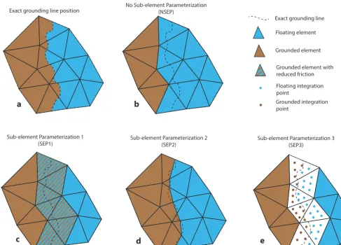
Figure 1. Grounding line discretization. Grounding line exact location (a), no sub-element parameterization (NSEP, b), sub-element
param-eterization 1 (SEP1, c), sub-element paramparam-eterization 2 (SEP2, d) and sub-element paramparam-eterization 3 (SEP3, e).
The position of the grounding line is determined by a floatation criterion: ice is floating if its thickness,H, is equal or lower than the floating heightHfdefined as follows:
Hf= −
ρw
ρi
r, r <0, (3)
whereρi is the ice density,ρw the ocean density and r the bedrock elevation (negative if below sea level). Grounding line is therefore located whereH=Hf:
H > Hf ice is grounded, (4)
H=Hf grounding line position, (5)
H < Hf ice is floating. (6)
2.2 Domain discretization
The domain is discretized with a 2-D isotropic uniform un-structured triangle mesh. Velocity and geometry fields are computed on each vertex of the mesh using Lagrange P1 (piecewise linear) finite elements. Element size varies be-tween 5 km for the lowest resolution and 250 m for the high-est resolution and is uniform within each mesh.
Grounding line position (Fig. 1a) is based on the hydro-static equilibrium condition as described above and three dif-ferent techniques are used to parameterize its position. As the same SSA equations are used on the entire domain to com-pute the stress balance, the only difference between grounded and floating ice is the presence or absence of basal friction.
In the first method, each element of the mesh is either grounded or floating: floatation criterion is determined on each vertex of the triangle and if at least one vertex of the triangle is floating, the element is considered floating and no friction is applied. Otherwise, if the three vertices are grounded, the element is considered grounded. This is the simplest approach used by fixed grid models to determine grounding line positions (Vieli and Payne, 2005), in which the grounding line is defined as the last grounded point. We refer to this technique as no sub-element parameterization (NSEP, Fig. 1b).
In the second method, the floating condition is a 2-D field and the grounding line position is determined by the line whereH=Hf, so it is located anywhere within an element.
2078 H. Seroussi et al.: Grounding line parameterization Some elements are therefore partly grounded and partly
float-ing. In this case the initial basal frictionCis reduced to match the amount of grounded ice in the element as proposed by Pattyn et al. (2006) and Gladstone et al. (2010a) but for a 2-D element:
Cg=C
Ag
A, (7)
whereCgis the applied basal friction coefficient for the el-ement partially grounded,Agis the area of grounded ice of this element and Ais the total area of the element. As all fields and data are computed using piecewise linear function, the grounding line position within each triangle is a straight line. This technique is referred to as sub-element parameter-ization 1 (SEP1, Fig. 1c) in the remainder of the paper.
In the third method, the grounding line position is located anywhere within an element as for SEP1, but the basal fric-tion computed for partly grounded elements differs. We take advantage of finite element properties to integrate the basal friction only on the part of the element that is grounded. This can be done simply by changing the integration area from the initial element to the grounded part of the element, over which the basal friction is unchanged. This technique is re-ferred to as sub-element parameterization 2 (SEP2, Fig. 1d) in the remainder of the manuscript.
In the fourth method, the sub-element parameterization is based on the number of integration points. We test the perfor-mance of this method by looking at the steady-state ground-ing line position (see experiments description below) for spa-tial resolutions of 1 and 5 km. The finite element method consists of calculating integrals over each element using a given set of integration points, also called Gaussian quadra-ture (Zienkiewicz and Taylor, 1989). The number of integra-tion points in each element depends on the degree of polyno-mial functions being integrated, with more integration points required for polynomial functions of higher degree. In our case, the basal friction goes from zero on the floating part of the element to the value specified in the experiment sec-tion, so this step function would require an infinite number of integration points to be exact. An alternative to the two SEP described above is to increase the number of integration points in the integrals and include basal friction for integra-tion points whose thickness is higher than the floating height. SEP3 only allows a finite number of grounding line positions to be captured within the element contrary to the other two SEP. We tested this alternative solution on the 1 and 5 km meshes, with integration orders going from 2 to 20, which is equivalent to a number of integration points varying be-tween 3 and 79. This technique is referred to as sub-element parameterization 3 (SEP3, Fig. 1e).
Appendix A details the different descriptions of the stiff-ness matrix associated to basal friction for all the sub-element parameterizations.
3 Experiments
We reproduce the MISMIP3D setup (Pattyn et al., 2013) and run similar experiments to investigate the influence of spatial resolution and grounding line parameterization on grounding line position and migration. Ice flows over a bedrock with a constant downward sloping bed that varies only in thex di-rection. The bedrock elevation is defined as follows:
b(x, y)= −100−x. (8)
Ice viscosity parameter, B, is uniform over the whole do-main and equal to 2.15×10⁸Pa s−1/3; the basal friction co-efficient,C, is also uniform for all grounded ice and equal to 107Pa m−1/3s1/3, soCis constant over each element ex-cept for those containing the grounding line, where it varies linearly; the friction law exponent,mis equal to 1/3. The domain is rectangular and stretches between 0 and 800 km in thex direction and 0 and 50 km in the y direction. The boundary conditions applied are as follows: a symmetric ice divide is considered atx=0 so the velocity is equal to zero. Water pressure is applied at x=800 km to model contact with the ocean. There is a symmetry axis aty=0 that repre-sents the centerline of the ice stream and a free slip condition fory=50 km, so there is no flux advected through these sur-faces and the tangential velocity is equal to zero.
Starting from a thin layer of ice of 10 m, a constant accu-mulationa˙ of 0.5 m yr−1is applied over the whole domain. The marine ice sheet evolves until a steady state configura-tion is reached. At each time step, we compute the ice veloc-ity, its thickness, the new grounding line position and update the upper and lower surfaces.
This steady state configuration is then perturbed by chang-ing the basal friction coefficientC. This parameter is adjusted spatially using a Gaussian bump such that
C∗=C
"
1−0.75 exp −(x−xb)
2
2x2 c
−(y−yb)
2
2y2 c
!#
, (9)
withC∗as the new friction coefficient,xbas the grounding line position at y=0 km in the steady state configuration,
yb=0,xc=150 km, andyc=10 km as the spatial extent of the perturbation along thex andy directions. The model is run forward in time for 100 years. The sliding friction is then reset to its initial uniform value and the model runs for-ward in time until a new steady state configuration is reached. This experiment is designed to assess the ability of models to provide reversible grounding line positions under simplified conditions (Pattyn et al., 2013). The marine ice sheet theory states that ice resting on a down sloping bed without lateral variations exhibits only one steady state grounding line posi-tion (Schoof, 2007b). MISMIP benchmark demonstrated that failure to reproduce the reversibility test is often associated with coarse mesh resolution.
H. Seroussi et al.: Grounding line parameterization 2079
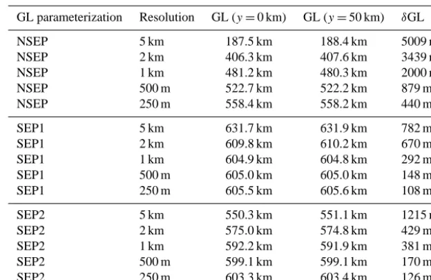
Table 1. Initial grounding line position and span for the NSEP, SEP1 and SEP2 simulations.
GL parameterization Resolution GL (y=0 km) GL (y=50 km) δGL
NSEP 5 km 187.5 km 188.4 km 5009 m
NSEP 2 km 406.3 km 407.6 km 3439 m
NSEP 1 km 481.2 km 480.3 km 2000 m
NSEP 500 m 522.7 km 522.2 km 879 m
NSEP 250 m 558.4 km 558.2 km 440 m
SEP1 5 km 631.7 km 631.9 km 782 m
SEP1 2 km 609.8 km 610.2 km 670 m
SEP1 1 km 604.9 km 604.8 km 292 m
SEP1 500 m 605.0 km 605.0 km 148 m
SEP1 250 m 605.5 km 605.6 km 108 m
SEP2 5 km 550.3 km 551.1 km 1215 m
SEP2 2 km 575.0 km 574.8 km 429 m
SEP2 1 km 592.2 km 591.9 km 381 m
SEP2 500 m 599.1 km 599.1 km 170 m
SEP2 250 m 603.3 km 603.4 km 126 m
Seroussi et al.: Grounding line parameterization 9
Exact grounding line position
Sub-element Parameterization 1
(SEP1) Sub-element Parameterization 2(SEP2) No Sub-element Parameterization
(NSEP)
a
d e
b
Sub-element Parameterization 3 (SEP3)
c
Exact grounding line
Grounded element with reduced friction Grounded element Floating element
Floating integration point
Grounded integration point
Fig. A1.Grounding line discretization. Grounding line exact location (a), no sub-element parameterization (NSEP, b), sub-element
parame-terization 1 (SEP1, c), sub-element parameparame-terization 3 (SEP2, d) and sub-element parameparame-terization 3 (SEP3,e).
5000 2000 1000 500 250 100
200 300 400 500 600 700
Resolution (m)
GL position (km)
Fig. A2. Steady state grounding line position iny= 0as a function of mesh refinement for NSEP (blue stars), SEP1 (green crosses) and
SEP2 (red circles).
Figure 2. Steady state grounding line position iny=0 as a function of mesh refinement for NSEP (blue stars), SEP1 (green crosses) and SEP2 (red circles).
from 5 km to 250 m, for a number of elements varying be-tween 2553 and 1 013 894 depending on the spatial resolu-tion. The first three grounding line parameterizations (NSEP, SEP1 and SEP2) are run for all mesh resolutions, resulting in a total of 15 simulations. The last grounding line param-eterization (SEP3) is only run to find the initial steady state grounding line position for meshes of 5 km and 1 km resolu-tion, with a varying number of integration points (19 simula-tions for each mesh resolution).
4 Results
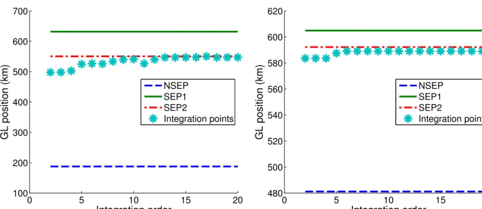
We consider that steady state is reached when the rate of change in ice thickness, grounding line position and ice velocity are all respectively lower than 10−5m yr−1, 10−3m yr−1and 10−5m yr−2, respectively. It takes approx-imately 50 000 years to reach steady state. We need to en-sure the Courant–Friedrichs–Lewy condition (CFL, Courant et al., 1967) for all models, so meshes with finer resolution require smaller time steps than the ones with coarser reso-lution. The initial grounding line position for each of the NSEP, SEP1 and SEP2 models is summarized in Table 1. It varies betweenx=188 km andx=632 km depending on the model resolution and grounding line parameterization. In the case of NSEP, the grounding position varies by several hundreds of kilometers (between 188 and 558 km), while SEP1 and SEP2 lead to variations in steady state ground-ing line positions of 50 km or less (between 605 and 632 km and between 550 and 603 km, respectively for the SEP1 and SEP2). This spread in grounding line positions is larger than in Feldmann et al. (2014). Steady state grounding line posi-tions aty=0 km for these three parameterizations and all mesh resolutions are shown on Fig. 2. Grounding line is moving upstream as the mesh resolution increases for SEP1, while it is moving downstream for NSEP and SEP2. Steady-state grounding line positions found with SEP3 are in good agreement with SEP2 for both 5 and 1 km mesh resolutions. It varies betweenx=540 andx=497 km, andx=584 and
x=589 km for mesh resolutions of 5 and 1 km, depending on the integration order (see Fig. 5), which is respectively within 10 and 3 km of SEP2 for a similar resolution when using enough integration points.
As for the domain configuration, the model parameteriza-tion and forcings do not vary in they direction and we have
2080 H. Seroussi et al.: Grounding line parameterization
uy(x,0)=uy(x,50)=0, the grounding line position should
therefore be a straight line parallel to theyaxis. In practice, this position slightly varies with y, especially since we use an unstructured mesh. We define the grounding line span as follows:
δGL=max xgi−min xgi, (10)
wherexgiare all grounding line positions for 0< y <50 km. The grounding line span is presented in Table 1 and provides a quantification of the spread of grounding line positions.
δGL is about twice the size of the elements for NSEP and less than half this size for SEP1 and SEP2.
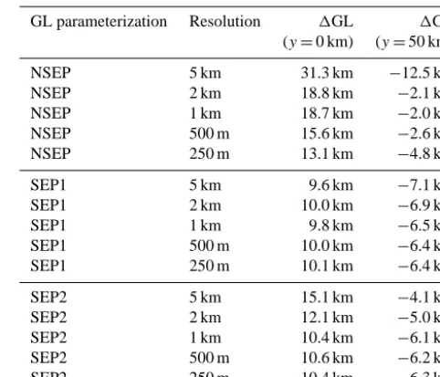
The perturbation experiment is performed to analyze the reversibility of the grounding line position in a simplified configuration. Figure 3 shows that grounding line advances along the glacier centerline as the basal friction is reduced in this area, and retreats along the free slip boundary. Advance and retreat extents vary depending on grounding line parame-terizations and mesh resolutions. Distances of advance along the centerline and retreat along the free-slip boundary after 100 years for all 15 simulations are presented in Table 2. Advances are more pronounced and retreats are reduced at low resolutions, except for SEP1 that exhibits similar ad-vance and retreat for all mesh sizes. Both SEP1 and SEP2 present advance and retreat after 100 years that converged toward 10 and 6.5 km respectively at high resolution.
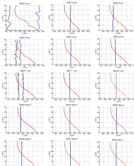
The updated steady state position reached after the per-turbation experiment is identical to the initial steady state position (Fig. 3), except for NSEP simulations at low reso-lution (more than 1 km resoreso-lution), so most simulations ex-hibit reversibility. The difference between the initial and fi-nal grounding line position is less than 10 m in all the cases where the two steady state grounding line positions superim-pose on Fig. 3.
To analyze the motion of the grounding line during the per-turbation experiment, Fig. 4 presents the 100 year advance and first 100 year retreat of the grounding line position dur-ing the basal perturbation experiment for the different res-olutions and grounding line parameterizations. Migration of grounding line position for y=0 and y=50 km is shown (one value every year). For NSEP (first column), grounding line position advances and retreats in discrete steps that are linked to the element size. For both SEP1 and SEP2 (sec-ond and third columns), the advance and retreat are contin-uous. Grounding line advance at y=50 km takes between 20 and 40 years to reach its most advanced position. In the case of NSEP, the grounding position remains stable after the advance, while for SEP1, SEP2 and NSEP at 250 m resolu-tion, it is followed by a small retreat. Grounding line retreat aty=0 km takes longer than the advance aty=50 km and is still evolving after 100 years in most cases, which shows that the grounding line is still far from having reached a new steady state position.
Table 2. Grounding line displacement during the perturbation
ex-periment for the 15 simulations.
GL parameterization Resolution 1GL 1GL (y=0 km) (y=50 km)
NSEP 5 km 31.3 km −12.5 km
NSEP 2 km 18.8 km −2.1 km
NSEP 1 km 18.7 km −2.0 km
NSEP 500 m 15.6 km −2.6 km
NSEP 250 m 13.1 km −4.8 km
SEP1 5 km 9.6 km −7.1 km
SEP1 2 km 10.0 km −6.9 km
SEP1 1 km 9.8 km −6.5 km
SEP1 500 m 10.0 km −6.4 km
SEP1 250 m 10.1 km −6.4 km
SEP2 5 km 15.1 km −4.1 km
SEP2 2 km 12.1 km −5.0 km
SEP2 1 km 10.4 km −6.1 km
SEP2 500 m 10.6 km −6.2 km
SEP2 250 m 10.4 km −6.3 km
5 Discussion
H. Seroussi et al.: Grounding line parameterization 2081
10 Seroussi et al.: Grounding line parameterization
1850 190 195 200 205 210 215 220 225 10 20 30 40 50 x (km) y (km)
NSEP 5 km
615 620 625 630 635 640 645 650
0 10 20 30 40 50 x (km) y (km)
SEP1 5 km
540 545 550 555 560 565 570 575
0 10 20 30 40 50 x (km) y (km)
SEP2 5 km
3950 400 405 410 415 420 425 430 435 10 20 30 40 50 x (km) y (km)
NSEP 2 km
595 600 605 610 615 620 625 630
0 10 20 30 40 50 x (km) y (km)
SEP1 2 km
560 565 570 575 580 585 590 595
0 10 20 30 40 50 x (km) y (km)
SEP2 2 km
470 475 480 485 490 495 500 505
0 10 20 30 40 50 x (km) y (km)
NSEP 1 km
590 595 600 605 610 615 620 625
0 10 20 30 40 50 x (km) y (km)
SEP1 1 km
575 580 585 590 595 600 605 610
0 10 20 30 40 50 x (km) y (km)
SEP2 1 km
510 515 520 525 530 535 540 545
0 10 20 30 40 50 x (km) y (km)
NSEP 500 m
590 595 600 605 610 615 620 625
0 10 20 30 40 50 x (km) y (km)
SEP1 500 m
585 590 595 600 605 610 615 620
0 10 20 30 40 50 x (km) y (km)
SEP2 500 m
545 550 555 560 565 570 575 580
0 10 20 30 40 50 x (km) y (km)
NSEP 250 m
590 595 600 605 610 615 620 625
0 10 20 30 40 50 x (km) y (km)
SEP1 250 m
585 590 595 600 605 610 615 620 625 0 10 20 30 40 50 x (km) y (km)
SEP2 250 m
Fig. A3.Initial steady state grounding line positions in the (x,y) plane (black line), position 100 years after the basal perturbation is introduced (red line) and new steady state position after the basal friction is reset to its initial value (blue line). Where black line is not visible, black and blue lines superimpose. x and y axis have the same scale for all plots.
Figure 3. Initial steady state grounding line positions in the (x,y) plane (black line), position 100 years after the basal perturbation is introduced (red line) and new steady state position after the basal friction is reset to its initial value (blue line). Where black line is not visible, black and blue lines superimpose.xandyaxis have the same scale for all plots.
2082Seroussi et al.: Grounding line parameterization H. Seroussi et al.: Grounding line parameterization11
0 20 40 60 80 100 190 195 200 205 210 215 time (yr)
GL position (km)
NSEP 5 km
0 20 40 60 80 100 620 625 630 635 640 645 650 time (yr)
GL position (km)
SEP1 5 km
0 20 40 60 80 100 545 550 555 560 565 570 time (yr)
GL position (km)
SEP2 5 km
0 20 40 60 80 100 400 405 410 415 420 425 time (yr)
GL position (km)
NSEP 2 km
0 20 40 60 80 100 600 605 610 615 620 625 time (yr)
GL position (km)
SEP1 2 km
0 20 40 60 80 100 565 570 575 580 585 590 time (yr)
GL position (km)
SEP2 2 km
0 20 40 60 80 100 475 480 485 490 495 500 505 time (yr)
GL position (km)
NSEP 1 km
0 20 40 60 80 100 595 600 605 610 615 620 625 time (yr)
GL position (km)
SEP1 1 km
0 20 40 60 80 100 585 590 595 600 605 610 time (yr)
GL position (km)
SEP2 1 km
0 20 40 60 80 100 515 520 525 530 535 540 time (yr)
GL position (km)
NSEP 500 m
0 20 40 60 80 100 595 600 605 610 615 620 625 time (yr)
GL position (km)
SEP1 500 m
0 20 40 60 80 100 590 595 600 605 610 615 time (yr)
GL position (km)
SEP2 500 m
0 20 40 60 80 100 550 555 560 565 570 575 time (yr)
GL position (km)
NSEP 250 m
0 20 40 60 80 100 595 600 605 610 615 620 time (yr)
GL position (km)
SEP1 250 m
0 20 40 60 80 100 595 600 605 610 615 620 time (yr)
GL position (km)
SEP2 250 m
Fig. A4.Time-dependent position of the grounding line along the symmetry axis (y= 0) and the free slip border (y= 50) during (respectively light red and dark red) and after (respectively light teal and dark teal) the friction perturbation for coarse mesh resolutions. y axes have the same scale for all simulations. x axes (time) is after the perturbation experiment (teal lines)
Figure 4. Time-dependent position of the grounding line along the symmetry axis (y=0) and the free slip border (y=50) during (respec-tively light red and dark red) and after (respec(respec-tively light teal and dark teal) the friction perturbation for coarse mesh resolutions.yaxes have the same scale for all simulations.xaxes (time) is reversed after the perturbation experiment (teal lines).
shows a similar behavior to a smaller extent, with a ground-ing line position located around 580 km.
The results presented here show that proper grounding line parameterization is crucial for marine ice sheet simulations as discrepancies of several tens of kilometers exist between
H. Seroussi et al.: Grounding line parameterization 2083 performed with different stress balance approximations in
Pattyn et al. (2013), demonstrating the critical impact of SEP. For example at 500 m resolution, the steady-state ground-ing line position varies between 522 and 605 km for NSEP and SEP1 respectively, so more than 80 km. In Pattyn et al. (2013), the same grounding line position computed with FS and hybrid L1L2 models (Hindmarsh, 2004) varies by less than 10 km, and by up to 80 km between FS and SSA models. Some previous results on flow-band models (Gladstone et al., 2010a) exhibit unstable behavior in grounding line re-treat in the case of NSEP. We did not experience this kind of behavior and all simulations were stable and converged to a steady state position. Grounding line advance and retreat was also continuous and located anywhere within the ele-ment, with no sign of preferred position within the element as observed in Gladstone et al. (2010a) when using SEP1 and SEP2. The second horizontal dimension of our model and the unstructured nature of our mesh may explain these differences.
As expected, grounding line span, δGL, is higher than model resolution for the NSEP while it is less than half of the model resolution for SEP1 and SEP2 (see Table 1). Dif-ferences in grounding line position between models based on a 500 and 250 m mesh resolution is respectively 25, 0.5 and 3.2 km for NSEP, SEP1 and SEP2. This suggests that ground-ing line position has not converged for NSEP, while the con-vergence error is 0.5 and 3.2 km respectively for the SEP1 and SEP2, as defined in Gladstone et al. (2010a, b).
In the reversibility test, all models except NSEP at a res-olution equal or higher than 1 km satisfy the reversibility condition. Numerical requirement to satisfy the reversibil-ity criterion is therefore a resolution below 1 km for NSEP; whereas all models based on sub-element parameterization exhibit reversibility even when relying on a coarse mesh. These results are consistent with Feldmann et al. (2014): re-versibility is observed for grid resolutions lower than 2 km for NSEP and with grid resolutions as low as 16 km when SEP is applied. The reversibility criterion is a however nec-essary condition that provides insights in the numerical as-pects of the marine ice sheet model and the simulations, but this test can be passed at relatively low resolutions for which steady-state grounding line positions are not accurate. It therefore does not guarantee the accuracy of the numerical treatment of the grounding line and sufficient mesh resolu-tion, as suggested by the large number of our simulations that verify the reversibility with different steady state grounding line positions.
If we compare SEP1 and SEP2, Fig. 2 shows that they both converge towards the same position for fine mesh resolutions, but that positions at coarser resolutions are upstream of the “converged” position for SEP1, and downstream for SEP2. The dynamic advance is also slightly different: grounding line advance at y=0 km is faster and goes farther for the SEP1. It is also associated to a larger retrograde retreat in the second part of the experiment, which is especially
pronounced at low resolutions. The grounding line retreat aty=50 km is also larger for SEP1 at low resolution, but both exhibit similar behaviors for resolutions finer than 2 km. A mesh resolution finer than 2 km should therefore be em-ployed to accurately capture dynamic behavior or marine ice sheet in this configuration. SEP2 is a more “exact” solution, as basal friction is integrated over the exact grounded part of the element, while SEP1 uses an area scaling of the basal friction. In this experiment, the basal friction is uniform over the whole domain, so it is not surprising that SEP1 and SEP2 lead to similar results. We expect greater differences to ap-pear in the case where basal friction varies over the domain, but this is beyond the scope of this paper.
SEP3 was tested only to find the steady-state position of the grounding line on the 5 and 1 km meshes. This method only allows a finite number of grounding line positions to be captured within the element contrary to the other two SEP. We tested this solution with integration orders going from 2 to 20. Results in Fig. 5 show that increasing the number of Gauss points only have an impact on grounding line position for coarse mesh resolutions. For the 1 km mesh, integration with order of 4 or below leads to one position, and integration with order of 5 and above leads to a second position; how-ever, the grounding line position is within 3 km of the SEP2. For the 5 km mesh, the spread in grounding line positions is much larger, with steady-state grounding line positions vary-ing by more than 50 km. If the integration order is greater than 12, however, these positions is located within 10 km of the SEP2 position. Increasing the number of integration points is therefore a simple solution to include basal friction in a portion of the element in a finite element framework, and provides results similar to other sub-element parameteriza-tions if the integration order is sufficient. This method should be further investigated using a larger range of mesh resolu-tions to ensure convergence of the grounding line position at finer mesh resolutions.
The results presented in this paper were all performed us-ing a 2-D SSA model and unstructured uniform isotropic meshes. Refinement away from the grounding line is impor-tant to accurately capture shear margins (Raymond, 1996) or topography that varies over short distances, but should not be uniform and be based, for example, on the Hessian of the ve-locity (Morlighem et al., 2010). Increasing mesh resolution has a double impact on computational time. First, increas-ing the number of degrees of freedom increases computa-tional time, mainly when solving the linear systems. Second, as the elements are smaller, the time steps allowed in tran-sient simulations in order to fulfill the CFL condition are re-duced. Fine mesh resolution is therefore necessary in critical areas but alternatives less computationally intensive should also be explored. Adding grounding line parameterizations is a simple improvement as grounding line positions are better captured at no additional cost. Sub-element parameterization allows grounding line position to be anywhere within an ele-ment, but the shape of the grounding line is still constrained
2084 H. Seroussi et al.: Grounding line parameterization
12
Seroussi et al.: Grounding line parameterization
0 5 10 15 20
100 200 300 400 500 600 700
Integration order
GL position (km)
NSEP SEP1 SEP2
Integration points
0 5 10 15 20
480 500 520 540 560 580 600 620
Integration order
GL position (km)
NSEP SEP1 SEP2
Integration points
Fig. A5. Grounding line position iny= 0for 5 km (left) and 1 km (right) resolution mesh for NSEP (dark blue dashed line), SEP1 (green
straight line), SEP2 (red dash dotted line) and SEP3 with different integration orders (light blue stars).
Figure 5. Grounding line position iny=0 for 5 km (left panel) and 1 km (right panel) resolution mesh for NSEP (dark-blue dashed line), SEP1 (green straight line), SEP2 (red dash dotted line) and SEP3 with different integration orders (light blue stars).
by the mesh resolution: exact grounding line position within an element remains a straight line if piecewise linear ele-ments are used. Mesh refinement and parameterizations are therefore two methods that should be combined.
This study shows that different grounding line parame-terizations lead to different grounding line steady state po-sitions as well as different dynamic behaviors. Differences in model simulations performed with and without SEP are as large as differences between models relying on different ice flow approximations in the MISMIP3D results (Pattyn et al., 2013), which demonstrate the importance of ground-ing line parameterization. We expect our results to be similar for higher-order (HO) models (Blatter, 1995; Pattyn, 2003). This is because HO models are similar to SSA (HO models include vertical shear stress as well), and the grounding line position is based on the hydrostatic condition in both cases. Models that do not include sub-element parameterizations will need a significantly finer mesh resolution to converge, and the grounding line position may likely be located further upstream than those based on a sub-element parameteriza-tion. Recent studies show that relying on full-Stokes in some critical areas in the model domain is necessary (Hindmarsh, 2004; Gudmundsson, 2008; Morlighem et al., 2010), and that grounding line position is better resolved using a contact me-chanics condition in this case (Nowicki and Wingham, 2008; Durand et al., 2009b). This condition, however, is only eval-uated on the edge or face on which the stress tensor is com-puted, and no SEP has yet been formulated for such models. This may explain why a very fine resolution on the order of tens of meters must be employed to model grounding line dynamics with FS in some cases (Durand et al., 2009b).
6 Conclusions
H. Seroussi et al.: Grounding line parameterization 2085 Appendix A: Description of basal friction integration
We detail here the stiffness matrices associated to basal fric-tion on grounded ice for the different sub-element parame-terizations. Let V be the space of kinematically admissible velocity fields and8=(φx, φy)∈Va kinematically
admis-sible velocity field. For any8∈Vthe stiffness matrix in the case of NSEP is
Kf= Z
0g
Cub·8d0, (A1)
where0bis the lower surface of the ice sheet where ice is grounded.
Using a decomposition over the elements and using inte-gration points to calculate the integral gives
Kf= X
Eg
X
g
Cub(g)·8(g)Wg, (A2)
whereEgare the grounded elements,gthe integration points used for the integration andWgthe weight associated to each integration point.
For SEP1, the friction coefficient is affected by the grounded area of each element, so the stiffness matrix is Kf=
X
Eg
X
g
Cgub(g)·8(g)Wg, (A3)
whereCg, Eq. (7), is the applied basal friction coefficient for elements partially grounded (Cg=C for elements com-pletely grounded).
For SEP2, the friction is applies only on the grounded part of the element, so the domain of integration is changed toEeg instead ofEg:
Kf= X
e
Eg
X
g
Cub(g)·8t (g)Wg, (A4)
whereEegcorresponds exactly to the brown area on Fig. 1d. In the code, this is done by creating sub-regions within each element partly grounded by determining the exact location of the points whereH=Hfand changing the integration do-main over these sub-regions.
For SEP3, the stiffness matrix is changed to Kf=
X
Eg
X
g
Cδ(g)ub(g)·8(g)Wg, (A5)
whereδ(g)is evaluated at each integration point:
δ(g)=
1 if H > Hf
0 if H≤Hf. (A6)
2086 H. Seroussi et al.: Grounding line parameterization
Acknowledgements. H. Seroussi was supported by an
appoint-ment to the NASA Postdoctoral Program at the Jet Propulsion Laboratory, administered by Oak Ridge Associated Universities through a contract with NASA. This work was performed at the Jet Propulsion Laboratory, California Institute of Technology, and at the Department of Earth System Science, University of California Irvine. A. Khazendar and M. Morlighem were supported by grants from the National Aeronautics and Space Administration’s Cryospheric Sciences Program. E. Larour was supported by grants from NASA’s Cryospheric Sciences and Modeling, Analysis and Prediction Programs. We thank R. Gladstone, F. Pattyn, G. Durand and A. Levermann for their suggestions which improved the quality of the manuscript.
Edited by: O. Gagliardini
References
Blatter, H.: Velocity And Stress-Fields In Grounded Glaciers: A Simple Algorithm For Including Deviatoric Stress Gradients, J. Glaciol., 41, 333–344, 1995.
Bohlander, J. and Scambos, T.: Antarctic coastlines and grounding line derived from MODIS Mosaic of Antarctica (MOA), digital media, Natl. Snow and Ice Data Cent., Boulder, 2007.
Cornford, S., Martin, D., Graves, D., Ranken, D. F., Le Brocq, A. M., Gladstone, R., Payne, A., Ng, E., and Lipscomb, W.: Adaptive mesh, finite volume modeling of marine ice sheets, J. Comput. Phys., 232, 529–549, doi:10.1016/j.jcp.2012.08.037, 2013.
Courant, R., Friedric, K., and Lewy, H.: On Partial Difference Equations Of Mathematical Physics, Ibm J. Res. Develop., 11, 215–234, 1967.
Cuffey, K. and Paterson, W. S. B.: The Physics of Glaciers, 4th Edn., Elsevier, Oxford, 2010.
Durand, G., Gagliardini, O., de Fleurian, B., Zwinger, T., and Le Meur, E.: Marine ice sheet dynamics: Hystere-sis and neutral equilibrium, J. Geophys. Res., 114, 1–10, doi:10.1029/2008JF001170, 2009a.
Durand, G., Gagliardini, O., Zwinger, T., Le Meur, E., and Hind-marsh, R.: Full Stokes modeling of marine ice sheets: influence of the grid size, Ann. Glaciol., 50, 109–114, 2009b.
Favier, L., Durand, G., Cornford, S. L., Gudmundsson, G. H., Gagliardini, O., Gillet-Chaulet, F., Zwinger, T., Payne, A. J., and Le Brocq, A.: Retreat of Pine Island Glacier controlled by marine ice-sheet instability, Nat. Clim. Change, 4, 117–121, doi:10.1038/NCLIMATE2094, 2014.
Feldmann, J., Albrecht, T., Khroulev, C., F., P., and Levermann, A.: Resolution-dependent performance of grounding line motion in a shallow model compared with a full-Stokes model accord-ing to the MISMIP3d intercomparison, J. Glaciol., 60, 353–359, doi:10.3189/2014JoG13J093, 2014.
Gladstone, R. M., Lee, V., Vieli, A., and Payne, A. J.: Grounding line migration in an adaptive mesh ice sheet model, J. Geophys. Res., 115, 1–19, doi:10.1029/2009JF001615, 2010a.
Gladstone, R. M., Payne, A. J., and Cornford, S. L.: Parameterising the grounding line in flow-line ice sheet models, The Cryosphere, 4, 605–619, doi:10.5194/tc-4-605-2010, 2010b.
Goldberg, D., Holland, D. M., and Schoof, C.: Grounding line movement and ice shelf buttressing in marine ice sheets, J. Geo-phys. Res., 114, 1–23, doi:10.1029/2008JF001227, 2009. Goldstein, R., Engelhardt, H., Kamb, B., and Frolich, R.: Satellite
Radar Interferometry for Monitoring ice-sheet motion: Applica-tion to an antarctic ice stream, Science, 262, 1525–1530, 1993. Gudmundsson, G. H.: Analytical solutions for the surface
re-sponse to small amplitude perturbations in boundary data in the shallow-ice-stream approximation, The Cryosphere, 2, 77–93, doi:10.5194/tc-2-77-2008, 2008.
Hindmarsh, R.: A numerical comparison of approximations to the Stokes equations used in ice sheet and glacier modeling, J. Geo-phys. Res., 109, 1–15, doi:10.1029/2003JF000065, 2004. Hindmarsh, R. and Le Meur, E.: Dynamical processes involved in
the retreat of marine ice sheets, J. Glaciol., 47, 271–282, 2001. Huybrechts, P.: A 3-D model for the Antarctic ice sheet: a
sensi-tivity study on the glacial-interglacial contrast, Clim. Dynam., 5, 79–92, 1990.
Katz, R. F. and Worster, M.: Stability of ice-sheet grounding lines, P. Roy. Soc. A, 466, 1597–1620, doi:10.1098/rspa.2009.0434, 2010.
Larour, E., Seroussi, H., Morlighem, M., and Rignot, E.: Continen-tal scale, high order, high spatial resolution, ice sheet modeling using the Ice Sheet System Model (ISSM), J. Geophys. Res., 117, 1–20, doi:10.1029/2011JF002140, 2012.
MacAyeal, D.: Large-scale ice flow over a viscous basal sediment: Theory and application to Ice Stream B, Antarctica, J. Geophys. Res., 94, 4071–4087, 1989.
Morlighem, M., Rignot, E., Seroussi, H., Larour, E., Ben Dhia, H., and Aubry, D.: Spatial patterns of basal drag inferred using con-trol methods from a full-Stokes and simpler models for Pine Island Glacier, West Antarctica, Geophys. Res. Lett., 37, 1–6, doi:10.1029/2010GL043853, 2010.
Nowicki, S. M. J. and Wingham, D. J.: Conditions for a steady ice sheet-ice shelf junction, Earth Planet. Sc. Lett., 265, 246–255, 2008.
Pattyn, F.: A new three-dimensional higher-order thermomechani-cal ice sheet model: Basic sensitivity, ice stream development, and ice flow across subglacial lakes, J. Geophys. Res., 108, 1–15, doi:10.1029/2002JB002329, 2003.
Pattyn, F. and Durand, G.: Why marine ice sheet model predictions may diverge in estimating future sea level rise, Geophys. Res. Lett., 40, 4316–4320, doi:10.1002/grl.50824, 2013.
Pattyn, F., Huyghe, A., De Brabander, S., and De Smedt, B.: Role of transition zones in marine ice sheet dynamics, J. Geophys. Res.-Earth, 111, 1–10, doi:10.1029/2005JF000394, 2006.
Pattyn, F., Schoof, C., Perichon, L., Hindmarsh, R. C. A., Bueler, E., de Fleurian, B., Durand, G., Gagliardini, O., Gladstone, R., Goldberg, D., Gudmundsson, G. H., Huybrechts, P., Lee, V., Nick, F. M., Payne, A. J., Pollard, D., Rybak, O., Saito, F., and Vieli, A.: Results of the Marine Ice Sheet Model Intercomparison Project, MISMIP, The Cryosphere, 6, 573–588, doi:10.5194/tc-6-573-2012, 2012..
H. Seroussi et al.: Grounding line parameterization 2087
Wilkens, N.: Grounding-line migration in plan-view marine ice-sheet models: results of the ice2sea MISMIP3d intercomparison, J. Glaciol., 59, 410–422, doi:10.3189/2013JoG12J129, 2013. Raymond, C.: Shear margins in glaciers and ice sheets, J. Glaciol.,
42, 90–102, 1996.
Rignot, E., Mouginot, J., and Scheuchl, B.: Antarctic grounding line mapping from differential satellite radar interferometry, Geo-phys. Res. Lett., 38, 1–6, doi:10.1029/2011GL047109, 2011a. Rignot, E., Velicogna, I., van den Broeke, M., Monaghan, A., and
Lenaerts, J.: Acceleration of the contribution of the Greenland and Antarctic ice sheets to sea level rise, Geophys. Res. Lett., 38, 1–5, doi:10.1029/2011GL046583, 2011b.
Ritz, C., Rommelaere, V., and Dumas, C.: Modeling the evolution of Antarctic ice sheet over the last 420,000 years: Implications for altitude changes in the Vostok region, J. Geophys. Res., 106, 31943–31964, doi:10.1029/2001JD900232, 2001.
Schodlok, M., Menemenlis, D., Rignot, E., and Studinger, M.: Sensitivity of the ice-shelf/ocean system to the sub-ice-shelf cavity shape measured by NASA IceBridge in Pine Is-land Glacier, West Antarctica, Ann. Glaciol., 53, 156–162, doi:10.3189/2012AoG60A073, 2012.
Schoof, C.: Marine ice-sheet dynamics. Part 1. The case of rapid sliding, J. Fluid Mech., 573, 27–55, doi:10.1017/S0022112006003570, 2007a.
Schoof, C.: Ice sheet grounding line dynamics: Steady states, stability, and hysteresis, J. Geophys. Res., 112, 1–19, doi:10.1029/2006JF000664, 2007b.
van der Veen, C.: Response of a Marine Ice-Sheet to Changes at the Grounding Line, Quaternary Res., 24, 257–267, doi:10.1016/0033-5894(85)90049-3, 1985.
Vieli, A. and Payne, A.: Assessing the ability of numerical ice sheet models to simulate grounding line migration, J. Geophys. Res., 110, 1–18, doi:10.1029/2004JF000202, 2005.
Weertman, J.: Stability of the junction of an ice sheet and an ice shelf, J. Glaciol., 13, 3–11, 1974.
Winkelmann, R., Martin, M. A., Haseloff, M., Albrecht, T., Bueler, E., Khroulev, C., and Levermann, A.: The Potsdam Parallel Ice Sheet Model (PISM-PIK) – Part 1: Model description, The Cryosphere, 5, 715–726, doi:10.5194/tc-5-715-2011, 2011. Zienkiewicz, O. C. and Taylor, R. L.: The finite element method,
vol. 1, 4th Edn., New York, London, 1989.