www.atmos-meas-tech.net/5/2827/2012/ doi:10.5194/amt-5-2827-2012
© Author(s) 2012. CC Attribution 3.0 License.
Measurement
Techniques
Six years of mesospheric CO estimated from ground-based
frequency-switched microwave radiometry at 57
◦
N compared with
satellite instruments
P. Forkman1, O. M. Christensen1, P. Eriksson1, J. Urban1, and B. Funke2
1Department of Earth and Space Sciences, Chalmers University of Technology, Sweden 2Instituto de Astrof´ısica de Andaluc´ıa (CSIC), Spain
Correspondence to: P. Forkman ([email protected])
Received: 29 March 2012 – Published in Atmos. Meas. Tech. Discuss.: 1 June 2012 Revised: 29 October 2012 – Accepted: 31 October 2012 – Published: 20 November 2012
Abstract. Measurements of mesospheric carbon monoxide, CO, provide important information about the dynamics in the mesosphere region since CO has a long lifetime at these altitudes. Ground-based measurements of mesospheric CO made at the Onsala Space Observatory, OSO, (57◦N, 12◦E) are presented. The dataset covers the period 2002–2008 and is hence uniquely long for ground-based observations. The simple and stable 115 GHz frequency-switched radiometer, calibration method, retrieval procedure and error character-ization are described. A comparison between our measure-ments and co-located CO measuremeasure-ments from the satellite sensors ACE-FTS on Scisat (v2.2), MLS on Aura (v3-3), MIPAS on Envisat (V3O CO 12 + 13 and V4O CO 200) and SMR on Odin (v225 and v021) is carried out. Our instrument, OSO, and the four satellite instruments show the same gen-eral variation of the vertical distribution of mesospheric CO in both the annual cycle and in shorter time period events, with high CO mixing ratios during winter and very low amounts during summer in the observed 55–100 km altitude range. During 2004–2008 the agreement of the OSO instru-ment and the satellite sensors ACE-FTS, MLS and MIPAS (200) is good in the altitude range 55–70 km. Above 70 km, OSO shows up to 25 % higher CO column values compared to both ACE and MLS. For the time period 2002–2004, CO from MIPAS (12 + 13) is up to 50 % lower than OSO be-tween 55 and 70 km. Mesospheric CO from the two versions of SMR deviates up to±65 % when compared to OSO, but the analysis is based on only a few co-locations.
1 Introduction
Above the tropopause, CO is formed in the upper meso-sphere/thermosphere mainly by photo-dissociation of CO2
and the major sink is by reactions with hydroxyl, OH. The vertical volume mixing ratio of middle atmospheric CO is characterized by low values in the stratosphere and a steep vertical gradient in the mesosphere.
and attributed variations in the CO column density to break-ing wave activity in the mesosphere. de Zafra and Muscari (2004) used 230 GHz observations of CO as a tracer of polar mesospheric dynamics. Kasai et al. (2005) made the first CO observations using ground-based solar absorption infrared spectroscopy, Velazco et al. (2007) made a long record of strato-mesospheric CO column values using the same tech-nique. Long-term CO measurements at both 115 GHz (Fork-man et al., 2003b) and infrared wavelengths (Borsdorff and Sussmann, 2009) have been compared with data from the Whole Atmosphere Community Climate Model, WACCM. Forkman et al. (2005) used CO measurements to estimate the vertical motion of the global circulation. Burrows et al. (2007) estimated horizontal mesospheric winds at Antarc-tica by the Doppler shift of ground-based microwave CO measurements. Hoffmann et al. (2011) compared ground-based CO measurements at 230 GHz with different satellite sensors.
The Improved Stratospheric and Mesospheric Sounder (ISAMS) onboard the Upper Atmosphere Research Satellite (UARS) made the first global stratospheric and lower meso-spheric CO measurements during 6 months in 1991–1992 (Allen et al., 1999). During the last ten years, several dif-ferent satellite sensors have been observing mesospheric CO including the microwave limb sounders SMR/Odin (Dupuy et al., 2004) and MLS/Aura (Pumphrey et al., 2007), the sun tracking ACE-FTS/Scisat-1 (Clerbaux et al., 2008) and the infrared limb sounder MIPAS/Envisat (Funke et al., 2009).
The lowest rotational transition of CO is at 115 GHz. The advantage of observing at 115 GHz compared to higher fre-quency transitions is both that the troposphere is optically thinner at lower frequencies and that pressure broadening ex-ceeds Doppler broadening up to about 70 km altitude, mak-ing it possible to estimate vertical profiles of CO up to this altitude and column values above.
Dicke-switching, i.e. signal-reference switching of the re-ceiver, is the standard microwave observation method in or-der to reduce the effect of gain drift in the receiver sys-tem. The intensities of the signal (the sky) and the reference (normally a blackbody load) have to balance each other to neutralize system gain nonlinearities. Frequency-switching, a small shift in the local oscillator frequency between the signal and reference phases, is a Dicke-switching variant. This method is mainly useful for the study of narrow lines like mesospheric CO at 115 GHz. One of the advantages of frequency-switching is that the line is present in both the sig-nal and the reference phases, which doubles the effective ob-servation time compared to “load-switching” where the ref-erence is a blackbody load. The frequency-switching observ-ing technique is commonly used in radio astronomy but more seldom used in microwave remote sensing.
In this study we present ground-based, frequency-switched measurements of mesospheric CO made at the On-sala Space Observatory, OSO, (57.4◦N, 11.9◦E). This is the longest ground-based measurement series of mesospheric
CO and covers the period 2002–2008. The instrument, cali-bration and inversion methods are described and the results are compared with data from four satellite instruments. Sec-tion 2 introduces our frequency-switched receiver system, Sect. 3 describes the inversions, Sect. 4 presents our results, Sect. 5 covers the satellite comparisons, and Sect. 6 gives a summary and the conclusions.
2 Measurement
2.1 Instrument and observation technique
Microwave remote sensing permits resolved line measure-ments of pure rotational transitions, which are sufficiently optically thin to allow observations from the ground. These lines are pressure-broadened in the atmosphere, and there-fore the measured shape of the spectrum contains informa-tion on the number density of the emitting constituent as a function of pressure. Information of the vertical distribution of the emitting constituent can be estimated using mathemat-ical inversion techniques (see Sect. 3).
We present measurements of CO made by a spectral, frequency-switched, heterodyne receiver used for the CO 1→0 transition at 115.27120 GHz based on a cooled Schot-tky single-sideband mixer. A block diagram of the receiver is shown in Fig. 1 and technical specifications are given in Ta-ble 1. The spectrometer is a 2-bit autocorrelator with 20 MHz bandwidth and 800 delay channels giving a nominal resolu-tion of 25 kHz.
In the frequency-switched radiometer, the local oscilla-tor is tuned between the signal and reference measurements. The intensities of the signal and reference phases balances each other as long as the frequency throw is small (normally
<10 MHz). If the frequency is switched,±1f the observed spectral feature will appear both as a negative and a pos-itive peak separated by 21f in the spectra. Since we use
1f= 4 MHz in the frequency-switching we have 8 MHz be-tween the peaks as seen in Fig. 2. If the observed spectral feature is narrower than 21f it will not be affected by the switching. Frequency-switching can be performed at high speed (5 Hz), which will remove faster gain variations than traditional load-switching.
2.2 Calibration
Horn Mixer IF Amp
20 K cryostat Hot load
Cold load N2 77 K Signal / Reference
PLL Gunn
Harm. mixer
* 60 * 4
Osc 1 Osc 2 Multipliers
A.C. Spectrometer Isolator
Computer
LO Band pass
Mirror
Oscillators
Local oscillator chain Lens
Fig. 1. Block diagram of the 115 GHz CO receiver system. The cold load is regularly mounted and used. Since the hot-cold calibrations are performed ahead of the lens, the losses in the lens and in the other components (horn, mixer, etc) along the transmission line are corrected for.
Table 1. Receiver specifications.
Radio frequency 115.261–115.281 GHz, SSB Mirror edge taper −35 dB
Elevation 90◦, fixed Cryostat window Teflon lens
Horn Aluminium, corrugated Beam width, FWHM (lens included) 3◦
First stage Cooled Schottky mixer, 20 K Image sideband rejection Mechanical back short Image sideband suppression >20 dB
Local oscillator (LO) Gunn oscillator LO frequency 111.27 GHz Frequency throw (21f) 8 MHz Mixer IF 4.0±0.3 GHz Total receiver temperature ∼325 K
Backend spectrometer 800 channel autocorrelator Bandwidth 20 MHz
Nominal resolution 25 kHz
minimizes Doppler shift effects due to horizontal movement of mesospheric air.
In microwave radiometry the intensity is normally pre-sented as brightness temperature, Tb. The receiver output
power is calibrated in units of antenna temperature,Ta. The
antenna temperature is the sky brightness temperature distri-bution weighted with the antenna radiation pattern. Since the beam is quite narrow and the sky brightness temperature in-creases only slowly, when the elevation changes from zenith to lower elevations (Forkman et al., 2003a) the zenith pencil beamTbcan be well approximated with the measuredTa.
The net power reaching the spectrometer consists of two components. The first one is proportional to the sky
−5 0 5 10
−0.4 −0.2 0 0.2 0.4
Frequency [MHz]
Brightness Temperature [K]
−5 0 5 10
−2 −1 0 1 2
Frequency [MHz]
Brightness Temperature [K]
−5 0 5 10
−0.4 −0.2 0 0.2 0.4
Frequency [MHz]
Brightness Temperature [K]
−5 0 5 10
−2 −1 0 1 2
Frequency [MHz]
Brightness Temperature [K]
Fig. 2. To the left: measured spectra (4 h average) with retrieval fits. To the right: residuals (measured spectrum–fit). The frequencies are given relative to the CO line center. The negative and positive peaks are the result of the frequency throw in the frequency-switching method. The spectra are corrected for baseline features. Note the weak CO signal in the summer (bottom figures).
brightness temperature. The other component is the power generated in the receiver system (lens, horn, mixer, etc), which we identify as the receiver temperature, Trec. The
sum of these components is the system temperature,Tsys=
Tb+Trec.
To estimateTrec, two blackbody loads with brightness
tem-peraturesThot (ambient load) andTcold(77 K load) are
ob-served each month. These hot-cold calibrations indicate that the variability ofTrecis less than 5 %.
Before each 15 min observation cycle, a calibration is per-formed to estimate the zenith sky brightness temperature. This is done by observing the zenith sky and an ambient load
Phot−Psky
Psky
=(Thot+Trec)−(Tb(z0)+Trec)
Tb(z0)+Trec
, (1)
wherePhotandPskyare the measured powers observing the
hot load and the zenith sky respectively,Tb(z0)is the zenith
sky brightness temperature (observed from the ground,z0).
Tb(z0)can be derived from the equation above sinceThotand
Trecare known.
Then during the observation cycle we record
1Tb(z0)=Tb(z0, f+)−Tb(z0, f−)
= 1P
Phot−Psky
(Thot−Tb(z0)), (2)
where1Tb(z0)is the difference in brightness temperatures
between the two frequenciesf +1f andf−1f, 1P is the difference between the measured powers at the two fre-quencies. Phot, Psky, Thot and Tb(z0) are taken from the
2.3 The tropospheric correction
Assuming a 1-layer model for the troposphere, the mi-crowave radiative transfer equation for a ground-based, zenith-looking observer can be written as
Tb(z0)=Tb(ztrop)e−τ+Ttrop(1−e−τ), (3)
where Tb(ztrop) is the brightness temperature as observed
from the tropopause, τ is the tropospheric zenith opacity andTtrop is the effective brightness temperature of the
tro-posphere. IfTtrop andτ are considered constant within the
frequency throw we get
1Tb(ztrop)=
1Tb(z0)
e−τ . (4)
In practiceτ is calculated from Eq. (3) as
τ= −ln T
trop−Tb(z0)
Ttrop−Tbg
. (5)
Since the atmospheric opacity is dominated by the contri-bution from the troposphere, the cosmic background radia-tion,Tbg, is used instead ofTb(ztrop)in Eq. (5). This means
that the calculatedτ actually is the atmospheric zenith opac-ity and hence includes the minor contribution from altitudes above the troposphere (e.g. absorption by stratospheric O2
and H2O).
The frequency-switching only yields 1Tb(z0), which is
close to zero except for the line peaks.Tb(z0)therefore has
to be measured separately as done in the calibration. To be able to estimate Ttrop in Eq. (5), one year of
radiosonde data from the Gothenburg-Landvetter Airport (37 km north-east of the observatory) have been processed in forward model calculations (Forkman et al., 2003a). Our esti-mation ofTtropis based on the correlation betweenTtropand
the ground temperature,Tgr, but we include the sky
bright-ness temperature,Tb(z0, ν), to improve the estimate.
Ttrop(ν)=αTgr+βTb(z0, ν), (6)
whereα=0.89 andβ=0.10 forν=115 GHz are found by applying the method of least squares to the processed ra-diosonde data. The error of theTtrop estimate was found to
be 3.5 K (1σ). CommonlyTtropis expressed as 0.95Tgr, but
the inclusion ofTb(z0)improves the estimate and reduces the
error by 10 %.
2.4 Calibration errors
An error in the estimate of the receiver temperature, Trec,
affects the estimation of the sky brightness temperature,
Tb(z0). If Trec is within the observed variation the error in
Tb(z0)should be less than 5 %. By comparing the thermal
noise,σtn, in the measured spectra with theoretical
calcula-tions, an estimate of the systematic calibration error can be
found.σtn in the spectra can be estimated by fitting a
poly-nomial to the measurement and calculating the standard de-viations of the residuals. By using the radiometric formula a theoretical estimate ofσtnis given by
σtn=
KTsys
√
t 1ν, (7)
wheretis the integration time,1νis the spectrometer resolu-tion andKdepends on the receiver type and configuration. In our caseKreduces to 1.15, which corresponds to the loss of information due to the digitalization of the signal (van Vleck clipping correction), see Rohlfs and Wilson (2008) for fur-ther details. By comparing these two calculations ofσtnwe
estimate the systematic error inTb(z0)to be less than 5 %.
If the measurement and the tropospheric correction are made in one step (Eqs. 2 and 4) it is clearly seen that errors in theTb(z0)estimation almost cancel out.
1Tb(ztrop)=
1P Phot−Psky
(Thot−Tb(z0))
Ttrop−Tbg
Ttrop−Tb(z0)
. (8) The error in 1Tb(ztrop) due to calibration and the
tropo-spheric correction is<2 %.
IfThotandTtropin Eq. (8) both are approximated with the
ambient temperature,TambandTambTbg, we get
1Tb(ztrop)=
1P Phot−Psky
Tamb, (9)
which describes the “chopper wheel” calibration method, which can be used for a quick but not so accurate calibration and correction for the tropospheric attenuation in one step.
In total we believe that the systematic errors from the mea-surements and the tropospheric corrections, including the effect of the variability of the tropospheric opacity within the measurement cycles, are within 5 % across the used bandwidth.
3 Retrievals
3.1 Terminology
The inversions were done using the Optimal Estimation Method (OEM) (Rodgers, 2000). The state of the atmosphere and instrument are described by a state vector, x. A
for-ward model, f, is then employed to mapx to a
measure-ment, y=f(x). The inverse problem consists in finding x given some measurement y. By linearizing the forward model y=Kx around the a priori atmosphere (xa), where
K is the Jacobian or weighting function matrix(∂y/∂x), the problem can be solved using linear algebra.
Doing this and applying OEM, the best estimate of the state vector is
ˆ
x=xa+(KTS−1K+S −1
a )
−1KTS−1
(y−f(xa))
where S is the covariance matrix describing the uncertainty in the measurement, Sathe covariance matrix for the a priori
profile and Gythe gain matrix. The relation between the true state, the a priori state and the retrieved state is given by
ˆ
x−x=(A−I)(x−xa)+GyKb(b− ˆb)
+Gy1f(x,b)+Gy, (11) where A is denoted the averaging kernel matrix, I is the iden-tity matrix,bandbˆ the true and estimated value of forward model parameter (i.e. line strength), Kbis the Jacobian ma-trix of the parameter (∂y/∂b), 1f(x,b) are errors in the forward model andx are errors in the measurement. For a complete definition and derivation see Rodgers (2000). The different terms will be discussed further in Sect. 4.1.
The AVK matrix is defined as A=∂xˆ/∂x. It describes the sensitivity of the retrieval to a change in the true state. Each element Aij gives the change in the retrieved profilexˆi, resulting from a perturbation in the true profilexj. A row in the AVK matrix can be regarded as a smoothing func-tion (averaging kernel) describing the vertical resolufunc-tion of the retrievals. The area of this smoothing function is called the measurement response and gives a rough indication of the contribution of the measurement to the retrieved value (Baron et al., 2002).
As mentioned in Hoffmann et al. (2011), the AVK will dif-fer in shape depending on whetherxis representing the vol-ume mixing ratio (VMR AVKs) or the relative change com-pared to the a priori concentration (fractional AVKs). Both type of AVKs will be presented in this paper for easier com-parison with other studies, however we will mainly use the VMR AVKs to characterize the instrument.
3.2 Retrieval setup
For the OSO inversions the forward model was provided by ARTS (v2.0) (Eriksson et al., 2011), and the retrieval software is a new version of Qpack (v2.0) (Eriksson et al., 2005). The retrieved quantities are CO volume mixing ratios, temperature, instrumental baselines and a frequency shift in the instrument. Only the CO VMR will be presented as a retrieval product, whereas the three others are retrieved mainly to stabilize the retrieval process. To ensure that the frequency shift is compensated for, the inversions were per-formed in an iterative leap using a Marquardt-Levenberg al-gorithm (Marks and Rodgers, 1993).
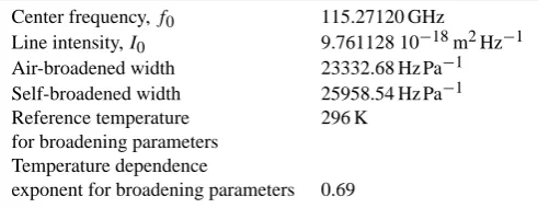
The spectroscopic line strength and position were taken from the JPL 2001 database (Pickett et al., 1998), whereas the pressure- and self-broadening parameters as well as their temperature dependence coefficients were taken from the HI-TRAN 2000 database (Rothman et al., 2003). Some of the used CO spectroscopic data are given in Table 2. Since the absorption of O2and H2O is compensated for in the
tropo-spheric correction (see Sect. 2.3) the only line included in the forward model calculations was the CO line at 115.27 GHz.
Table 2. Some of the used CO spectroscopic data.
Center frequency,f0 115.27120 GHz
Line intensity,I0 9.761128 10−18m2Hz−1
Air-broadened width 23332.68 Hz Pa−1
Self-broadened width 25958.54 Hz Pa−1
Reference temperature 296 K
for broadening parameters Temperature dependence
exponent for broadening parameters 0.69
The retrieval was performed on a pressure grid ranging from 2738 Pa (∼10 km) to 0.87 mPa (∼130 km), with a log-arithmic spacing of 0.125 decades (∼2 km).
The temperature and pressure data were taken from the MSIS90 climatology (Hedin, 1991), and the temperature a priori covariance matrix was given as a matrix with diagonal entries Sii=25 K (i.e. standard deviation of 5 K). Further-more, since the temperature in the real atmosphere is cor-related in altitude the non-diagonal elements Sij =σiσjρij were constructed so that the correlation (ρ) would decline linearly with a correlation of 0.37 when the altitude differ-ence (correlation length) betweeniandj was 4 km (roughly based on Eriksson, 2000).
The abundance of CO is highly variable over the year and OEM requires using the best estimate atmosphere as a priori. Therefore a monthly mean from a run of the Whole Atmo-sphere Community Climate Model (WACCM) (Garcia et al., 2007) was created and used as the a priori profile for the cen-ter day in each month. The value for other days were found by linearly interpolating onto each day. To simplify the error analysis, however, the covariance matrix for the a priori data was kept constant (in VMR) throughout the year.
Following Eriksson (2000), the covariance matrix for CO consists of two parts. The first represents the uncertainty of the mean a priori profile for each month. As with tempera-ture, the covariance matrix must also represent correlation in altitude for this error. This was modeled to decline linearly with a correlation length of 8 km. The standard deviation was set to 50 % of the yearly mean of the a priori profiles. The second part represents the natural variability of CO on shorter timescales which was set to 0.5 ppm for all altitudes and with no correlation between the layers.
The OSO instrument had problems with baseline features before an upgrade on 7 January 2004. After this upgrade the baseline variation was reduced significantly. To account for this, an instrumental baseline was retrieved by fitting a 5th order polynomial with a diagonal a priori covariance ma-trix with entries from 20 K (0th order) to 5 K (5th order) for dates before this upgrade, and entries from 20 K (0th order) to 0.05 K (5th order) for dates after this upgrade. This leads to a different measurement response for the different dates.
50 60 70 80 90 100 110
0 10 20 30 40
10−4
10−3
10−2
10−1
100
Pressure (hPa)
CO VMR (ppm) DJF
50 60 70 80 90 100 110
Approx altitude (km)
0 10 20 30 40
10−4
10−3
10−2
10−1
100
MAM
CO VMR (ppm)
50 60 70 80 90 100 110
0 10 20 30 40
10−4
10−3
10−2
10−1
100
Pressure (hPa)
JJA
CO VMR (ppm)
50 60 70 80 90 100 110
Approx altitude (km)
0 10 20 30 40
10−4
10−3
10−2
10−1
100
SON
CO VMR (ppm)
Fig. 3. Retrieved profiles 2002–2008 (every 20th profile is plotted for each season). CO volume mixing ratios are plotted against pres-sure (and altitude). The red line shows the average a priori profile for the season, and the dashed line the standard deviation of the a priori profile. Green lines are retrieved profiles 2002–2004 and the blue lines are profiles 2004–2008. The mean measurement response of the OSO instrument is higher than 0.8 between the black horizontal lines.
channel correlation of the thermal noise was measured to be 1.6 nominal channel widths, so S was given as a covari-ance matrix with a correlation length of 1.6 nominal channel widths. The magnitude of the thermal noise was estimated in each measurement independently by fitting a polynomial of order 3 to the measurement and calculating the RMS of the residuals at the wings.
4 Results of the OSO measurements
Figure 2 shows a sample spectrum, the corresponding re-trieved spectrum and the residuals for a typical winter and summer measurement. The CO line is much fainter during the summer than the winter line due to the strong seasonal cycle of CO (Sect. 1). The residuals are of equal strength, with both summer and winter showing that the system tem-perature is more or less constant during the year. Example profiles for each season are plotted in Fig. 3.
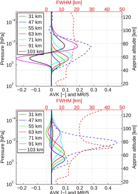
The shapes of the VMR AVKs are quite similar in both winter and summer. The most notable feature of the VMR AVKs is the negative values around 60 km for the AVKs cor-responding to retrieved values above 90 km (pink and black curves in Figs. 4 and 5). Although this looks dramatic, it is important to remember that these AVKs represent the sensi-tivity to changes in VMR. The concentration of CO is much lower at 60 km than above 90 km, and accordingly the ex-pected variability in CO VMR is also much lower. This im-plies that the impact of the negative lobes will be small, as the retrieved value follows the product of the AVK value and
the deviation from the a priori (see first term Eq. 11). The corresponding averaging kernels (the rows of AVK matrix) can be seen in Figs. 4 and 5.
Since CO has a very strong vertical gradient, relative changes at altitudes above the target altitude will give a larger effect than relative changes beneath. This changes the shape and area of the fractional AVKs, especially around 70 km during the summer where the fractional AVKs becomes ex-tremely wide. Here strong vertical gradients combined with poor vertical resolution even results in the measurement re-sponse of the fractional AVKs to become greater then one. This means that a concentration change of 10 % at one al-titude could give a responding change of 20 % at a lower altitude.
This complication is less prominent when using the VMR AVKs, rather than the fractional AVKs, to define the mea-surement response of the instrument. Note that the measure-ment response then describes the instrumeasure-ments’ sensitivity to changes in vmr rather than changes relative to the a priori. The use of VMR AVKs is motivated by the fact that the strong vertical gradient of CO combined with a meander-ing vortex can lead to extremely large changes in the true atmosphere relative to the a priori. This variation is easier to describe in VMR rather than relative units, and the sensitive range is therefore given as such. To further address the is-sue of the poor vertical resolution above 70 km, only the col-umn (rather than individual layers) will be used above this altitude.
The retrievals have an average degree of freedom (trace of the AVK matrix) of 1.8 before 2004 and 2.2 after 2004. The measurement response (VMR) is above 80 % approximately between 55 and 85 km. The vertical resolution within this altitude range is about 15–20 km (see Figs. 4 and 5). The beam of the OSO instrument has a horizontal width of about 4 km in the mesosphere.
The results presented in this paper will be given as the mix-ing ratios at 36 Pa (55 km), 12 Pa (63 km) and columns above 4 Pa (71 km) where Doppler broadening dominates. The col-umn values are calculated by summing up the number densi-ties from the air pressures below 4 Pa. The number densidensi-ties are calculated from the retrieved profiles using the a priori temperature profiles.
4.1 Errors
The error of the retrieval is the difference between the true state x and the retrieved state xˆ. The error can be divided into several parts corresponding to each term in Eq. (11).
−0.2 −0.1 0 0.1 0.2 0.3 0.4 10−4
10−2
100
102
AVK [−] and MR/5
Pressure [hPa]
31 km 47 km 55 km 63 km 71 km 91 km 103 km
0 10 20 30 40 50
20 40 60 80 100 120
FWHM [km]
Approx altitude [km]
−0.2 −0.1 0 0.1 0.2 0.3 0.4 10−4
10−2
100
102
AVK [−] and MR/5
Pressure [hPa]
31 km 47 km 55 km 63 km 71 km 91 km 103 km
0 10 20 30 40 50
20 40 60 80 100 120
FWHM [km]
Approx altitude [km]
Fig. 4. Solid lines show the averaging kernels from 27 Decem-ber 2005 in vmr (a) and fractional (b) units for different altitudes. The blue dash-dotted line is the measurement response divided by 5. The red dashed line shows the FWHM of the averaging kernels.
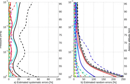
is taken into account by Eq. (12) and the smoothing error is thus ignored. The second term is the model parameter error, which describes the error in the retrieval arising from the dif-ference between the true value of a forward model parameter band the estimated valuebˆ. This will be discussed further in Sect. 4.2. The third term is the forward model error, which comes from direct errors in the forward model from either approximations or not modeled processes. This last term will not be discussed in this paper and is negligible. A thorough validation of ARTS is presented in Melsheimer et al. (2005). The last term is the retrieval noise, which is the error com-ing from noise in the measured spectra. It is described by the covariance matrix Sm=GySGTy. This error is random and will introduce noise into the retrieved profiles. An estimate of this noise is shown as the blue lines in Fig. 6. The dashed (dashed-dot) line shows the value for winter (summer) re-trievals and the solid line the mean retrieval noise. The big difference between summer and winter values is due to the low concentration of CO during summer.
−0.2 −0.1 0 0.1 0.2 0.3 0.4 10−4
10−2
100
102
AVK [−] and MR/5
Pressure [hPa]
31 km 47 km 55 km 63 km 71 km 91 km 103 km
0 10 20 30 40 50
20 40 60 80 100 120
FWHM [km]
Approx altitude [km]
−0.2 −0.1 0 0.1 0.2 0.3 0.4 10−4
10−2
100
102
AVK [−] and MR/5
Pressure [hPa]
31 km 47 km 55 km 63 km 71 km 91 km 103 km
0 10 20 30 40 50
20 40 60 80 100 120
FWHM [km]
Approx altitude [km]
Fig. 5. Solid lines show the averaging kernels from 26 June 2006 in vmr (a) and fractional (b) units for different altitudes. The blue dash-dotted line is the measurement response divided by 5. The red dashed line shows the FWHM of the averaging kernels.
4.2 Forward model parameter errors
In addition to the errors accounted for in the retrieval, there will be systematic errors from the forward model as well as instrumental errors which might influence the retrievals. To estimate the influence of errors in different retrieval parame-ters on the results, the retrievals from year 2006 were used. The summer values (JJA) were removed resulting in 177 re-maining spectra, which were rerun with the different parame-ters perturbed with their estimated 1σ-error. The differences between the standard and the perturbed inversions show that errors in forward model parameters can lead to a systematic error (bias) as well a decreased precision in each measure-ment. The systematic error can be described byxpert=k·xstd
at each altitude, wherexpertis the value of the perturbed
in-version,xstd the retrieved value using the standard
50 55 60 65 70 75 80 85 90 95
0 20 40 60 80 100
10−3
10−2
10−1
100
Pressure (hPa)
a) Estimated systematic errors [%]
50 55 60 65 70 75 80 85 90 95
Approx altitude (km)
0 50 100 150 200 250
10−3
10−2
10−1
100
b) Estimated random errors [%]
Fig. 6. In (a) the estimated systematic errors and in (b) the ran-dom errors. The colored (except blue) lines show the mean rela-tive change (a) and standard deviation (b) in the retrieved value at each altitude as the different forward model parameters are
per-turbed. The forward model parameters are: line-strength,I0,
(green-dashed), temperature profile,T, (cyan-dashed), pressure
broaden-ing parameter,γP, (yellow-dashed), temperature coefficient for the
broadening parameter,αP, (yellow-dashed-dot), a priori profile,xa,
(red-dashed-dot), 50 % a priori uncertainty,Sx, (green-dashed-dot),
removing natural variability from a priori uncertainty, Sx,
(red-solid), a priori uncertainty for the polynomial fit (cyan-dashed-dot), calibration errors (magenta-dashed-dot) and backend channel broadening error (cyan). The black line in both figures is the root-sum-square of the parameter errors. In (a) the black-dashed is the sum of the errors. The dark blue lines in (b) show the retrieval noise from 1 January 2006 (dashed), 2 September 2006 (dashed-dot) scaled with the a priori profile for the respective day as well as the average retrieval noise (solid). The black dashed line in (b) is the root-sum of the average retrieval noise (blue-solid) and the total parameter variability (black-solid).
the relative difference between the standard and perturbed inversions (i.e. scaled with the a priori).
The different forward model parameters tested include the line strength of the CO transition, the pressure broadening parameter and the instrument backend channel response. In addition, the a priori temperature profile, a priori CO profile, a priori uncertainty and size of the polynomial baseline fit were perturbed to test the possible systematic errors arising from different retrieval parameters.
For the spectral parameters the error estimates were done by comparing the values for HITRAN 2000, HITRAN 2008 and JPL 2001. If the discrepancies between the databases were bigger than the given error estimate in the database the discrepancy was used, if not the error estimate from the database was used. This gives a line strengthI0uncertainty of
1 % (JPL-database), a pressure broadening parameterγP un-certainty of 10 % (HITRAN 2000 unun-certainty) and an uncer-tainty in the temperature coefficientαPof the pressure broad-ening parameter of 10 % (difference between HITRAN 2000 and HITRAN 2008). Errors in the self-broadening parame-ters were found to be insignificant to the retrieval and will
not be presented in this paper. In total, the spectroscopic pa-rameters together give errors of less than 5 % in the retrievals. To investigate the influence of the calibration errors, the spectra were simply multiplied with 1±0.05 to simulate the 1σ calibration error (see Sect. 2.4). To test the influence of the a priori, the CO profile was perturbed by 50 % and the standard deviation for the a priori uncertainty covariance ma-trix was changed with 50 %. In addition, another test was done where the part representing the natural variability (0.5 ppm at all altitudes) was removed from the uncertainty ma-trix, and only the uncertainty in a priori mean was used. The temperature profile was perturbed by 5 K (1σ error for MSIS90 is 3 K) to take errors in temperature into account. The polynomial baseline fit in the retrieval had its a priori variance multiplied and divided by 4.
Figure 6a shows the estimated systematic error for the dif-ferent parameters and their root-sum-square (solid black). This estimate indicates the total systematic error expected in the measurements. The solid black line shows the sum of all the errors, this represents a worst case scenario for systematic errors which we will use before 2004.
In addition to the systematic errors, uncertainties in the forward model and retrieval parameters also lead to a de-creased precision. Figure 6b shows the standard deviation from each parameter and their root-sum-square (solid black). Combined (root-sum-square) with the average retrieval noise (blue solid) an estimate of the precision of the measurements is obtained and shown as the black dashed line in Fig. 6b.
The total estimated averaged systematic error between 55– 85 km is in the order of 15 % for profiles and 10 % for column values. The worst case error, the sum of the different errors, is of the order of 25 % for profiles and 20 % for the column values. Estimated average random errors between 55–85 km is 30–50 %, but is significantly worse when the concentra-tion of CO is low. The random errors mainly comes from the retrieval noise, and depend heavily on the a priori uncer-tainty at those altitudes (red curve Fig. 6), with a higher un-certainty leading to more noise. The retrieval noise from one such date (2 September 2006) is shown as the dashed-blue line in Fig. 6b.
5 Comparison
5.1 Satellite instruments
Table 3. Satellite and data characteristics.
Satellite instrument ACE-FTS Aura-MLS
Reference Clerbaux et al. (2008) Pumphrey et al. (2007) CO data version V 2.2 V-3-3
Measurement principle Sun tracking, absorption Limb sounding, emission Wavelength or frequency 2.3 & 4.7 µm 230 GHz
Launch 12 August 2003 15 July 2004 Orbit inclination 74◦ 90◦ Vertical range 6–100 km 16–80 km Vertical resolution (mesosphere) 4 km 7–8 km Horizontal resolution (mesosphere) 500 km 200 km Systematic errors (above 60 km) Better than±25 % ±20 %
Co-location range satellite-OSO <1500 km &<±20 % PV <1500km &<±20 % PV Co-located measurement days 126 618
Satellite instrument Envisat-MIPAS Odin-SMR Reference Funke et al. (2009) Dupuy et al. (2004) CO data version V3O(12 + 13) 2003–2004 V021 (new version) CO data version V4O(200) 2005–2008 V225 (old version) Measurement principle Limb sounding, emission Limb sounding, emission Wavelength or frequency 4.7 µm 576.4 GHz
Launch 1 March 2002 20 February 2001 Orbit inclination 98.6◦ 97.8◦
Vertical range 6–70 km 17–110 km Vertical resolution (mesosphere) 10 km 3 km Horizontal resolution (mesosphere) 500 km 500 km Systematic error (50–70km) ±10 % Not available
Co-location range satellite-OSO <1500 km &<±20 % PV <1500 km &<±20 % PV Co-located measurement days 418 22
characteristics of the four satellite sensors. As seen in Ta-ble 3, we use two different CO datasets for MIPAS and SMR. For MIPAS we use version V3O CO 12 and V3O CO 13 obtained from high spectral resolution measurements during 2003–2004 and version V4O CO 200 in the period 2005– 2008 when the MIPAS spectral resolution was reduced as consequence of an instrumental failure. All MIPAS observa-tions used here were taken in the nominal observation mode covering tangent heights within 6–70 km. For SMR we use both the older v225 and the newer v021. V021 is an extended dataset compared to v225 using all the available observa-tion modes. V225 has been used in previous comparisons (e.g. Clerbaux et al., 2008).
5.2 Comparison procedure
Side-looking satellites and a zenith-looking ground-based in-strument do not observe the same air volume. Comparisons between satellite- and ground-based instruments are there-fore complicated. All the satellites report data from a 100 times longer horizontal path than OSO but their vertical lution are up to four times better. Differences in vertical reso-lution can be compensated for by using the averaging kernels of the instruments but differences in horizontal resolution are harder to adjust for. A second issue is the co-location crite-rion to apply. At periods when small horizontal variations of CO are expected in the mesosphere (as in the summer)
2002 2004 2006 2008
−1 0 1 2 3
CO at 55 km [ppm]
Year
2002 2004 2006 20080
20 40 60
2 4 6 8 10 12
−1 0 1 2 3
Month
2 4 6 8 10 12 0
20 40 60
PVU at 55 km
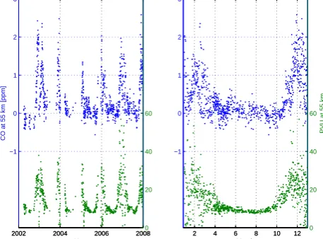
Fig. 7. CO volume mixing ratio and PV above OSO at 55 km alti-tude. To the left: the time series 2002–2008. To the right: the data from the different years stacked together. The modified Ertel’s PV
is used and 1 PVU = 10−6K m2s−1kg−1. The overall correlation
between CO and PV is 0.63.
within 1500 km radius from OSO and along the horizontal paths of the satellite beams. These deviations can partly be compensated for by using observed potential vorticity as a supplementary co-location criteria.
The polar vortex builds up in the autumn and breaks down in the spring. The potential vorticity (PV) of an air parcel is a measure of the position of the air parcel relative to the polar vortex. Figure 7 shows the OSO CO volume mixing ratio at 55 km together with the modified Ertel’s PV (Lait, 1994), cal-culated from the ECMWF operational dataset at 55 km dur-ing the time period 2002–2008. Figure 7 shows both a time series for the different years and the data for the different years stacked together to clearly see the seasonal variation. Both the CO mixing ratio and the PV have a steep and dis-tinct increase in the autumn. The winter is characterized by the meandering of the polar vortex, which brings in or out CO rich air from the polar region and this causes fast varia-tions of both CO mixing ratio and PV. The decrease in CO and PV in the spring is both less steep and less distinct than the increase in the autumn. The PV is low and stable in the summer and the CO mixing ratio is close to zero but show a high variability in the measurements. The high variability is explained by the faint CO signal in the summer which gives a low signal to noise ratio. The overall correlation between the CO mixing ratio and PV is 0.63.
The co-location criteria was chosen as follows: the tem-poral co-location criteria was set to the same date for satel-lite and OSO. The air volume measured by the satelsatel-lite had to be within a radius of 1500 km from OSO. The potential vorticity (PV) of the air volume measured by the satellite had to be within 20 % of the PV above OSO (Hoffmann et al., 2011 used a similar co-location procedure). The PV data were taken from the ECMWF operational data set at the potential temperature level of 2000 K (∼50 km altitude) and the modified Ertel’s PV (Lait, 1994) was calculated for both satellites and OSO. Figure 8 show the co-located positions for the four satellites.
For the comparison, the satellite data were interpolated onto the OSO retrieval grid. In the relevant vertical range the best resolution of the different satellites are roughly 4 km, which is about twice the interpolation resolution used. Hence the interpolation errors should be small (<1 %) which also is confirmed in a test (not shown).
For grid points outside the valid data points for the satel-lite the OSO a priori CO data were used. To take into account the different vertical resolution of the instruments the satel-lite data was convolved with the averaging kernels, A, of the OSO instrument (Rodgers and Connor, 2003)
xs=xa+A(xsat−xa), (12)
wherexsis the smoothed version of the satellite profilexsat,
andxais the OSO a priori profile.
ACE−FTS MLS−AURA
MIPAS Odin−SMR
ACE−FTS MLS−AURA
MIPAS Odin−SMR
MIPAS Odin−SMR
MIPAS Odin−SMR
Fig. 8. Satellite (co-location) positions. The dots indicate the satel-lite positions within 1500 km radius from OSO, which also ful-fill the PV criteria. In the MIPAS co-location map red/blue dots show (12 + 13)/(200) data, respectively. In the Odin co-location map red/blue show v225/v021, respectively.
5.3 Results of the satellite comparison
The satellite comparison is divided in the time periods: 2002– 2004 and 2004–2008. As mentioned in Sect. 3.2 there were baseline features in the OSO spectra 2002–2004 that may have affected the retrieved vertical profiles. These features disappeared when the local oscillator chain of the instru-ment was rebuilt in the beginning of 2004. Figure 9 shows time series of CO from OSO, MIPAS (12 + 13) and SMR (021 + 225) for the time period 2002–2004 and Fig. 10 show time series from OSO, ACE, MIPAS (200), MLS and SMR (225) for the time period 2004–2008. Both figures show CO volume mixing ratios at 55 and 63 km and column values above 71 km. No column values are presented for MIPAS and MLS since the nominal MIPAS CO observations are not vertically resolved above 70 km, and the upper limit for MLS is about 80 km. Figure 11 shows the WACCM mean CO vol-ume mixing ratio and the mean CO number densities. The main contribution for the column values is from altitudes
<100 km, even if the volume mixing ratio is increasing with altitude. This is explained by the exponential decrease in air pressure, and hence in air density, with altitude.
2003 2004 −1
0 1 2 3
CO VMR (ppm)
CO VMR at 36.5174 Pa ~ 55 km,
2003 2004
−1 0 1 2 3 4 5
CO VMR (ppm)
CO VMR at 11.5478 Pa ~ 63 km,
2003 2004
0 5 10 15x 10
19
CO total column (m
−2
)
CO total column above 3.6517 Pa ~ 71 km,
Fig. 9. Time series of CO mixing ratio at 55 km and 63 km and columns above 71 km for the time period 2002–2004 are shown: OSO (black), MIPAS (12 + 13, green plus), SMR (V021, brown cross; V225, brown stars) and a priori (cyan).
these figures is mainly the higher values of OSO compared to MIPAS ( 12 + 13) at 63 km (Fig. 9).
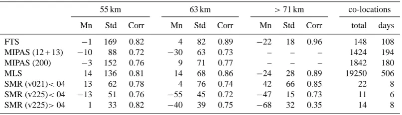
Figures 12–13 and Table 4 give a more detailed view of the comparison. Figure 12 shows the mean relative differences between the satellites and OSO for the time periods 2002– 2004 and 2004–2008. The differences are discussed for each satellite instrument later in this section.
Figure 13 shows the mean absolute and relative stan-dard deviations between OSO and the satellites. These de-viations originate from noise in the different instruments, from fluctuations due to insufficient co-location and forward model/retrieval parameters. Below 65 km the OSO measure-ment response gradually decreases, which explain the in-crease of the deviations below this altitude.
Table 4 gives a supplement to Figs. 12–13 showing the mean relative differences, the mean standard deviations and the mean correlation between OSO and the satellites. The correlation of the data from OSO and the satellite instruments is high.
The OSO summer CO spectra have a very low signal to noise ratio leading to a higher relative noise (Figs. 2b and 6). This gives a high variability in the retrieved summer mixing ratios (Fig. 10). The summer values are therefore excluded in Figs. 12–13 and Table 4 to avoid the noisy OSO summer measurements interference in the satellite comparison.
Taken into account the systematics errors of OSO (≤15 %) and the satellites (20–30 %, see Table 3) OSO overlaps the satellites in the time period 2004–2008 when OSO is com-pared to ACE, MIPAS (200) and MLS.
2005 2006 2007
−1 0 1 2 3
CO VMR (ppm)
CO VMR at 36.5174 Pa ~ 55 km,
2005 2006 2007
−1 0 1 2 3 4 5
CO VMR (ppm)
CO VMR at 11.5478 Pa ~ 63 km,
2005 2006 2007
0 5 10 15x 10
19
CO total column (m
−2
)
CO total column above 3.6517 Pa ~ 71 km,
Fig. 10. Time series of CO mixing ratio at 55 km and 63 km and columns above 71 km for the time period 2004–2008 are shown: OSO (black), FTS (blue cross), MIPAS (200, green plus), MLS (red dots), SMR (V225, brown stars) and a priori (cyan dashed).
0 2 4 6 8 10 12 14 16 18
20 40 60 80 100 120 140
CO number density [1015/m3]
Altitude [km]
0 10 20 30 40 50 60
20 40 60 80 100 120 140 CO volume mixing ratio [ppm]
Fig. 11. The number density of CO (black) and the volume mixing ratio of CO (red) versus altitude. The data shown are the mean sum-mer (solid) and mean winter (dashed) OSO a priori from WACCM. The main contribution to the column above 70 km originates from
altitudes≤100 km altitude.
5.3.1 ACE and MLS
50 55 60 65 70 75 80 85 90 95 50 55 60 65 70 75 80 85 90 95 50 55 60 65 70 75 80 85 90 95 50 55 60 65 70 75 80 85 90 95
Approx altitude (km)
−100 −50 0 50 100
10−3 10−2 10−1 100 Pressure (hPa) Sat−OSO 50 55 60 65 70 75 80 85 90 95 50 55 60 65 70 75 80 85 90 95 50 55 60 65 70 75 80 85 90 95 50 55 60 65 70 75 80 85 90 95 50 55 60 65 70 75 80 85 90 95
Approx altitude (km)
−100 −50 0 50 100
10−3 10−2 10−1 100 Pressure (hPa) Sat−OSO
Fig. 12. Mean relative differences between satellites and OSO; (Left): the time period 2002–2004, MIPAS (12 + 13, green), SMR (V021, dashed brown) and SMR (V225, solid brown). (Right): the time period 2004–2008, FTS(blue), MIPAS (200, green), MLS (red) and SMR (V225, brown). The deviating lengths of the satellite pro-files is explained by the different vertical coverage of the satellites. The shaded areas show the estimated systematic error of the differ-ent satellites. The vertical black lines are the estimated systematic errors of the OSO instrument, 2002–2004 the worst case systematic error is used due to baseline problems (see Sect. 4.2). The horizontal black dashed lines show the vertical limits of the OSO observations. The summer values are excluded.
Table 4 OSO has higher CO mixing ratios above 70 km com-pared to ACE and MLS leading to 25 % higher CO column values (>71 km). The MLS column values are close to the OSO a priori since the upper limit of MLS is about 80 km and we use the a priori CO data for grid points outside the vertical range of the satellite (see Sect. 5.2).
5.3.2 MIPAS
MIPAS (200) shows only a small deviation in CO mixing ra-tios compared to OSO. MIPAS (12 + 13) does not show the same good agreement when compared to OSO, it has up to 50 % lower values than OSO above 55 km. MIPAS (12 + 13) and MIPAS (200) have the same vertical coverage though MIPAS (200) is slightly better vertically sampled (due to shorter integration time). Resulting vertical resolutions of re-trieved profiles, however, are quite similar.
Up to March 2004 only MIPAS (12 + 13) data are avail-able and after March 2004 only MIPAS (200) data. In this comparison we have no overlap between MIPAS (12 + 13) and the other satellites except a few collocations with SMR (021 + 225). Clerbaux et al. (2008) compared CO data from the beginning of 2004 from MIPAS (9 + 10) and ACE and found that the CO mixing ratios from MIPAS (9 + 10) is within ±26 % of the ACE mixing ratios in the altitude range 55–70 km. The most probable reason for the deviation
50 55 60 65 70 75 80 85 90 95 50 55 60 65 70 75 80 85 90 95 50 55 60 65 70 75 80 85 90 95 50 55 60 65 70 75 80 85 90 95 50 55 60 65 70 75 80 85 90 95 50 55 60 65 70 75 80 85 90 95 50 55 60 65 70 75 80 85 90 95 50 55 60 65 70 75 80 85 90 95
0 1 2 3 4
10−3
10−2
10−1
100
Pressure (hPa)
STD(∆ x) [PPM]
50 55 60 65 70 75 80 85 90 95 50 55 60 65 70 75 80 85 90 95 50 55 60 65 70 75 80 85 90 95 50 55 60 65 70 75 80 85 90 95 50 55 60 65 70 75 80 85 90 95 50 55 60 65 70 75 80 85 90 95 50 55 60 65 70 75 80 85 90 95 50 55 60 65 70 75 80 85 90 95
Approx altitude (km)
0 50 100 150 200 250
10−3
10−2
10−1
100
STD(∆ x) [%] MIPASV30(12+13) OdinV021 OdinV225 FTS MLS MIPASV40(200) OdinV225
Fig. 13. The mean standard deviation between OSO and the satellites; absolute(left) and relative(right). MIPAS (12 + 13), SMR (v021), and the dotted SMR (v225) are from the time period 2002– 2004. The vertical coverage of the satellites explains the deviating extension of the profiles. The horizontal black dashed lines show the vertical limits of the OSO observations. The dashed line at 60 km is the lower limit 2002–2004 and the dash-dotted line at 55 km is the lower limit 2004–2008. The black line is the root-sum of the aver-age retrieval noise and the total forward model parameter variability of the OSO instrument. The summer values are excluded.
between OSO and MIPAS (12 + 13) can be the baseline fea-tures seen in the OSO spectra before 2004.
5.3.3 SMR
The two CO datasets of SMR deviate in different ways com-pared to the OSO data at 55–95 km. SMR (225) shows down to 65 % lower mixing ratios than OSO and SMR (021) shows up to 50 % higher mixing ratios (Fig. 12). A reason for the general discrepancy between SMR and OSO can be the few co-locations with OSO but this does not explain the differ-ence between the two SMR versions. V021 is regarded to be the more accurate than v225. Comparisons between SMR (021 + 225) and ACE shows the same general discrepancy between v225 and v021 (not shown).
6 Summary and conclusions
Ground-based, frequency-switched measurements of meso-spheric CO at 115 GHz from Onsala Space Observatory (57◦N, 12◦E) during the time period 2002–2008 are presented.
Table 4. Statistics for 55 km, 63 km and for total columns>71 km. Mn (%) the mean relative difference of CO between satellite and OSO
(>0 if the satellite reports more CO than OSO), Std (%) the mean standard deviations, Corr the mean correlation of CO between satellite
and OSO, total the total number of co-located measurements, days the number of days with co-located measurements. The summer values are excluded.
55 km 63 km >71 km co-locations
Mn Std Corr Mn Std Corr Mn Std Corr total days
FTS −1 169 0.82 4 82 0.89 −22 18 0.96 148 108
MIPAS (12 + 13) −10 88 0.72 −30 63 0.73 – – – 1424 194
MIPAS (200) −3 152 0.76 9 71 0.77 – – – 1842 180
MLS 14 136 0.81 14 68 0.86 −24 28 0.89 19250 506
SMR (v021)<04 13 62 0.78 4 76 0.74 42 66 0.85 22 8
SMR (v225)<04 −13 51 0.76 −55 45 0.72 −47 15 0.73 11 6
SMR (v225)>04 1 33 0.82 −40 39 0.75 −68 32 0.35 14 8
and gain variations are almost canceled out and that no time is spent observing a reference load. Frequency-switching is very well suited for the observation of narrow transition lines as in the case of mesospheric CO at 115 GHz.
The Optimal Estimation Method, OEM, has been used to retrieve vertical CO profiles from the measured spectra. A thorough error analysis has been performed to investigate the systematic effects due to the uncertainties in the different pa-rameters used in the measurement and retrieval process to give an as accurate error estimation as possible.
The OSO instrument has provided the longest time series of ground-based mesospheric CO measurements so far. The OSO data show the same general features as data from satel-lite instruments both in the annual cycle, characterized by high CO mixing ratios during winter and very low mixing ratios during summer, and in shorter time period events.
The OSO CO data have been compared to CO datasets from four satellite instruments; ACE-FTS (v2.2) on Scisat, MIPAS (V3O CO 12 + 13 and V4O CO 200) on Envisat, MLS (v3-3) on Aura and SMR (v225 and v021) on Odin.
A satellite measurement is assumed to be co-located with OSO if the measurement is done the same day and if the air at the tangent point of the satellite both is within a radius of 1500 km from OSO and deviates less than 20 % in PV (potential vorticity) compared to the air above OSO.
During the time period 2004–2008 the averaged CO datasets retrieved by OSO and ACE, MLS and MIPAS (200) do not differ by more than 15 % in the altitude range 55– 70 km, which is within the combined systematic errors of the different instruments (see Fig. 12b).
The time period 2002–2004 MIPAS (12 + 13) shows up to 50 % smaller mixing ratios compared to OSO. One reason for the observed difference between the OSO and MIPAS (12 + 13) mesospheric CO datasets can be due to baseline features seen in the OSO spectra before February 2004.
SMR (021 + 225) have very few co-located CO measure-ments with OSO. V225 shows up to 65 % lower mixing ra-tios than OSO and the v021 measurements show up to 50 % higher mixing ratios than OSO.
Above 70 km we compare the CO column values from OSO and the satellite sensors ACE, MLS and SMR. The OSO column values are about 25 % higher than the values from both ACE and MLS. SMR (021) shows up to 65 % higher column values than OSO. The MLS column values are close to the OSO a priori values since we use a priori information outside the vertical range of the satellite (the up-per vertical limit for MLS is 80 km). SMR has very few co-located measurements with OSO.
The systematic error above 70 km is±25 % for ACE and ±10 % for OSO. If the systematic errors for ACE and OSO are correctly estimated the mean true profile has to be in the range where the mean profiles of OSO and ACE (in-clusive their systematic errors) overlaps. Since ACE shows 25 % lower column values than OSO, this indicates that OSO has a positive bias of less than 10 % above 70 km and that ACE has a negative bias of about 15–25 % above 70 km (see Fig. 12b). Hoffmann et al. (2011) report an offset pattern when their ground-based instrument is compared to ACE and MLS, which is similar to the offset pattern we report when OSO is compared to the same satellites. Additional compar-isons of upper mesospheric CO are needed to understand the reason for this observed offset between ground-based and satellite instruments.
Observation of mesospheric CO provides important in-formation of the mesospheric dynamics. The satellite sen-sors which measure mesospheric CO today are not, to our knowledge, planned to be replaced when they stop function-ing. Therefore, in a few years, ground-based instruments will be even more important than today. The CO transition at 115 GHz is suitable for ground-based studies of the upper atmosphere due to both that the lower atmosphere is fairly transparent, at this frequency, and that pressure broadening exceeds Doppler broadening as high as 70 km, making it pos-sible to estimate vertical profiles up to this altitude and to estimate column values above.
115 GHz can be used as a low cost alternative to clarify this issue.
Acknowledgements. The Swedish Natural Science Research Council supported the maintenance and development of the OSO receiver system. We thank the teams behind HITRAN, JPL and WACCM for providing a priori information to the retrievals. We thank the community behind ARTS for software used in the retrieval process. We thank ECMWF for wind field data and the teams behind MLS/Aura, MIPAS/Envisat and ACE-FTS/SCISAT for providing the satellite CO datasets. The Atmospheric Chemistry Experiment (ACE), also known as SCISAT, is a Canadian-led mission mainly supported by the Canadian Space Agency and the Natural Sciences and Engineering Research Council of Canada. We also thank the Department of Earth and Space Sciences, Chalmers University of Technology for SMR/Odin CO data. Odin is a Swedish-led satellite project funded jointly by the Swedish National Space Board (SNSB), the Canadian Space Agency (CSA), the National Technology Agency of Finland (Tekes), the Centre National d’Etudes Spatiales (CNES) in France and the European Space Agency (ESA). We thank the laboratory and workshop of Onsala Space Observatory for keeping the OSO receiver up and running. Finally we thank the reviewers for their helpful comments on the manuscript.
Edited by: R. Sussmann
References
Aellig, C., Kaempfer, N., and Hauchecorne, A.: Variability of meso-spheric CO in the fall and winter as observed with ground-based microwave radiometry at 115 GHz, J. Geophys. Res., 100, 14125–14130, doi:10.1029/95JD00984, 1995.
Allen, D., Stanford, J., L´opez-Valverde, M., Nakamura, N.,
Lary, D., Douglass, A., Cerniglia, M., Remedios, J.,
and Taylor, F.: Observations of middle atmosphere CO from the UARS ISAMS during the early northern winter 1991/92, J. Atmos. Sci., 56, 563–583,
doi:10.1175/1520-0469(1999)056<0563:OOMACF>2.0.CO;2, 1999.
Baron, P., Ricaud, P., de La No¨e, J., Eriksson, P., Merino, F., and Murtagh, D.: Studies for the Odin sub-millimetre ra-diometer: Retrieval methodology, Can. J. Phys., 80, 341–356, doi:10.1139/P01-150, 2002.
Bevilacqua, R., Stark, A., and Schwartz, P.: The variability of car-bon monoxide in the terrestrial mesosphere as determined from
ground-based observations of theJ=1→0 emission line, J.
Geophys. Res., 90, 5777–5782, doi:10.1029/JD090iD03p05777, 1985.
Borsdorff, T. and Sussmann, R.: On seasonality of stratomeso-spheric CO above midlatitudes: New insight from solar FTIR spectrometry at Zugspitze and Garmisch, Geophys. Res. Lett., 36, 804, doi:10.1029/2009GL040056, 2009.
Burrows, S., Martin, C., and Roberts, E.: High-latitude remote sens-ing of mesospheric wind speeds and carbon monoxide, J. Geo-phys. Res., 112, 109, doi:10.1029/2006JD007993, 2007. Clancy, R., Muhleman, D., and Allen, M.: Seasonal variability of
CO in the terrestrial mesosphere, J. Geophys. Res., 89, 9673– 9676, doi:10.1029/JD089iD06p09673, 1984.
Clerbaux, C., George, M., Turquety, S., Walker, K. A., Barret, B., Bernath, P., Boone, C., Borsdorff, T., Cammas, J. P., Catoire, V., Coffey, M., Coheur, P.-F., Deeter, M., De Mazi`ere, M., Drum-mond, J., Duchatelet, P., Dupuy, E., de Zafra, R., Eddounia, F., Edwards, D. P., Emmons, L., Funke, B., Gille, J., Griffith, D. W. T., Hannigan, J., Hase, F., H¨opfner, M., Jones, N., Ka-gawa, A., Kasai, Y., Kramer, I., Le Flochmo¨en, E., Livesey, N. J., L´opez-Puertas, M., Luo, M., Mahieu, E., Murtagh, D., N´ed´elec, P., Pazmino, A., Pumphrey, H., Ricaud, P., Rinsland, C. P., Robert, C., Schneider, M., Senten, C., Stiller, G., Strandberg, A., Strong, K., Sussmann, R., Thouret, V., Urban, J., and Wiacek, A.: CO measurements from the ACE-FTS satellite instrument: data analysis and validation using ground-based, airborne and spaceborne observations, Atmos. Chem. Phys., 8, 2569–2594, doi:10.5194/acp-8-2569-2008, 2008.
de Zafra, R. and Muscari, G.: CO as an important high-altitude tracer of dynamics in the polar stratosphere and mesosphere, J. Geophys. Res, 109, D06105, doi:10.1029/2003JD004099, 2004.
Dupuy, E., Urban, J., Ricaud, P., Le Flochmo¨en, ´E., Lauti´e, N.,
Murtagh, D., De La No¨e, J., El Amraoui, L., Eriksson, P., Fork-man, P., Frisk, U., J´egou, F., Jim´enez, C., and Olberg, M.: Strato-mesospheric measurements of carbon monoxide with the Odin Sub-Millimetre Radiometer: Retrieval and first results, Geophys. Res. Lett., 31, L20101, doi:10.1029/2004GL020558, 2004. Eriksson, P.: Analysis and comparison of two linear regularization
methods for passive atmospheric observations, J. Geophys. Res., 105, 18157–18167, doi:10.1029/2000JD900172, 2000.
Eriksson, P., Jim´enez, C., and Buehler, S. A.: Qpack, a tool for in-strument simulation and retrieval work, J. Quant. Spectrosc. Ra., 91, 47–64, doi:10.1016/j.jqsrt.2004.05.050, 2005.
Eriksson, P., Buehler, S. A., Davis, C. P., Emde, C., and Lemke, O.: ARTS, the atmospheric radiative transfer simu-lator, Version 2, J. Quant. Spectrosc. Ra., 112, 1551–1558, doi:10.1016/j.jqsrt.2011.03.001, 2011.
Forkman, P., Eriksson, P., and Winnberg, A.: The 22 GHz Radio-aeronomy receiver at Onsala Space Observatory, J. Quant. Spectrosc. Ra., 77, 23–42, doi:10.1016/S0022-4073(02)00073-0, 2003a.
Forkman, P., Eriksson, P., Winnberg, A., Garcia, R., and Kinnison, D.: Longest continuous ground-based measure-ments of mesospheric CO, Geophys. Res. Lett., 30, 1532, doi:10.1029/2003GL016931, 2003b.
Forkman, P., Eriksson, P., and Murtagh, D.: Observing the vertical
branch of the mesospheric circulation at lat N60◦using ground
based measurements of CO and H2O, J. Geophys. Res., 110, 107,
doi:10.1029/2004JD004916, 2005.
Funke, B., L´opez-Puertas, M., Garc´ıa-Comas, M., Stiller, G. P., von Clarmann, T., H¨opfner, M., Glatthor, N., Grabowski, U., Kell-mann, S., and Linden, A.: Carbon monoxide distributions from the upper troposphere to the mesosphere inferred from 4.7 µm non-local thermal equilibrium emissions measured by MIPAS on Envisat, Atmos. Chem. Phys., 9, 2387–2411, doi:10.5194/acp-9-2387-2009, 2009.
Hedin, A. E.: Extension of the MSIS thermosphere model into the middle and lower atmosphere, J. Geophys. Res., 96, 1159–1172, doi:10.1029/90JA02125, 1991.
Hoffmann, C. G., Raffalski, U., Palm, M., Funke, B., Golchert, S. H. W., Hochschild, G., and Notholt, J.: Observation of strato-mesospheric CO above Kiruna with ground-based microwave radiometry – retrieval and satellite comparison, Atmos. Meas. Tech., 4, 2389–2408, doi:10.5194/amt-4-2389-2011, 2011. Kasai, Y. J., Koshiro, T., Endo, M., Jones, N. B., and Murayama,
Y.: Ground-based measurement of strato-mesospheric CO by a FTIR spectrometer over Poker Flat, Alaska, Adv. Space Res., 35, 2024–2030, doi:10.1016/j.asr.2005.04.099, 2005.
Lait, L.: An alternative form for potential vorticity,
J. Atmos. Sci., 51, 1754–1759,
doi:10.1175/1520-0469(1994)051<1754:AAFFPV>2.0.CO;2, 1994.
Lopez-Puertas, M., Lopez-Valverde, M., Garcia, R., and Roble, R.:
A review of CO2and CO abundances in the middle atmosphere,
Geoph. Monog., 123, 83–100, doi:10.1029/GM123p0083, 2000. Marks, C. and Rodgers, C.: A retrieval method for atmospheric composition from limb emission measurements, J. Geophys. Res., 98, 14939–14953, doi:10.1029/93JD01195, 1993. Melsheimer, C., Verdes, C., Buehler, S. A., Emde, C.,
Eriks-son, P., Feist, D. G., Ichizawa, S., John, V. O., Kasai, Y., Kopp, G., Koulev, N., Kuhn, T., Lemke, O., Ochiai, S., Schreier, F., Sreerekha, T. R., Suzuki, M., Takahashi, C., Tsu-jimaru, S., and Urban, J.: Intercomparison of general purpose clear sky atmospheric radiative transfer models for the mil-limeter/submillimeter spectral range, Radio Sci., 40, RS1007, doi:10.1029/2004RS003110, 2005.
Pickett, H., Poynter, R., Cohen, E., Delitsky, M., Pearson, J., and M¨uller, H.: Submillimeter, millimeter, and microwave spectral line catalog, J. Quant. Spectrosc. Ra., 60, 883–890, doi:10.1016/S0022-4073(98)00091-0, 1998.
Pumphrey, H. C., Filipiak, M., Livesey, N., Schwartz, M., Boone, C., Walker, K., Bernath, P., Ricaud, P., Barret, B., Clerbaux, C., Jarnot, R., Manney, G., and Waters, J.: Validation of middle-atmosphere carbon monoxide retrievals from MLS on Aura, J. Geophys. Res., 112, D24S38, doi:10.1029/2007JD008723, 2007. Rodgers, C. D.: Inverse methods for atmospheric sounding: Theory
and practice, World Scientific, Singapore, 2000.
Rodgers, C. D. and Connor, B.: Intercomparison of re-mote sounding instruments, J. Geophys. Res., 108, 4116, doi:10.1029/2002JD002299, 2003.
Rohlfs, K. and Wilson, T. L.: Tools of Radio Astronomy, Springer-Verlag, Berlin, 2008.
Rothman, L., Barbe, A., Chris Benner, D., Brown, L., Camy-Peyret, C., Carleer, M., Chance, K., Clerbaux, C., Dana, V., Devi, V., Devic, V., Fayt, A., Flaudi, J., Gamachej, R., Gold-man, A., Jacquemart, D., Jucks, K., Lafferty, W., Mandin, J., Massie, S., Nemtchinov, V., Newnham, D., Perrin, A., Rins-land, C., Schroeder, J., Smith, K., Smith, M., Tang, K., Toth, R., Vander Auwera, J., Varanasi, P., and Yoshino, K.: The HI-TRAN molecular spectroscopic database: edition of 2000 includ-ing updates through 2001, J. Quant. Spectrosc. Ra., 82, 5–44, doi:10.1016/S0022-4073(03)00146-8, 2003.
Velazco, V., Wood, S. W., Sinnhuber, M., Kramer, I., Jones, N. B., Kasai, Y., Notholt, J., Warneke, T., Blumenstock, T., Hase, F., Murcray, F. J., and Schrems, O.: Annual variation of strato-mesospheric carbon monoxide measured by ground-based Fourier transform infrared spectrometry, Atmos. Chem. Phys., 7, 1305–1312, doi:10.5194/acp-7-1305-2007, 2007.