Integrating Satellite-Derived Data as Spatial Predictors in Multiple Regression Models to Enhance the Knowledge of Air Temperature Patterns

(1)

Integrating Satellite-Derived Data as Spatial

Predictors in Multiple Regression Models to Enhance

the Knowledge of Air Temperature Patterns

Lucille Alonso * and Florent Renard *

UMR CNRS Environment City Society, University Jean Moulin Lyon 3, 69007 Lyon, France * Correspondence: [email protected] (L.A.); [email protected] (F.R.)

Received: 24 August 2019; Accepted: 17 September 2019; Published: 21 September 2019

Abstract: With the phenomenon of urban heat island and thermal discomfort felt in urban areas, exacerbated by climate change, it is necessary to best estimate the air temperature in every part of an area, especially in the context of the on-going rationalization weather stations network. In addition, the comprehension of air temperature patterns is essential for multiple applications in the fields of agriculture, hydrology, land development or public health. Thus, this study proposes to estimate the air temperature from 28 explanatory variables, using multiple linear regressions. The innovation of this study is to integrate variables from remote sensing into the model in addition to the variables traditionally used like the ones from the Land Use Land Cover. The contribution of spectral indices is significant and makes it possible to improve the quality of the prediction model. However, modeling errors are still present. Their locations and magnitudes are analyzed. However, although the results provided by modelling are of good quality in most cases, particularly thanks to the introduction of explanatory variables from remote sensing, this can never replace dense networks of ground-based measurements. Nevertheless, the methodology presented, applicable to any territory and not requiring specific computer resources, can be highly useful in many fields, particularly for urban planners.

Keywords: multiple linear regression; remote sensing; spectral indices; air temperature; urban heat island; land use land cover

1. Introduction

According to Météo-France’s regional models, temperature increases are expected to continue in France for decades to come [1]. Indeed, at the scale of the Rhône-Alpes region, the work of Météo France [2] and the results of regional climate models for Europe, integrating RCP (Representative Concentration Pathways) scenarios 4.5 and 8.5 of the Intergovernmental Panel on Climate Change foresees an increase in annual and seasonal temperatures [1]. Summer temperatures are expected to rise by between 0.5 and 2◦C by 2050 compared to the 1976–2005 reference period [3]. This results in a probability of heat waves increase and intensification. Indeed, the phenomena of regional heat waves are superimposed on the microclimatic features of local urban environments [4–6]. These heat waves are exacerbated in urban areas by the urban heat island phenomenon (UHI) [7]. This UHI concept refers to the observed temperature differences between urban and surrounding rural areas [8].

Consequently, accurate knowledge of temperatures is a necessity both for the environment and for health policies. This knowledge depends directly on the density of the measurement network. This is not a new phenomenon and multiple studies have studied this question, through classical spatial interpolations (deterministic [9] or stochastic [9,10]) or multiple regressions [11–15], for example. This issue is very important in the context of climate change and the rise of heat waves, particularly with the closure of several Météo-France measurement stations [16,17].

(2)

Several studies show the relative contribution of land use and land cover (LULC), topography data and urban typologies to UHI development [12,13,18]. However, very few studies tried to model air temperature using land surface temperature (LST) obtained from remote sensing data, like the NEX (NASA Earth Exchange) Gridded Daily Meteorology (NEX-GDM) model [19–21] over the United States. This study showed the importance of the spatially continuous data sets. In addition, no studies in France, to our knowledge, tried to incorporate into these models spectral indices or other products obtained for remote sensing, apart from LST, such as reflectance, Modified Normalized Difference Water Index (MNDWI), Normalized Difference Bareness Index (NDBaI) or Normalized Difference Moisture Index (NDMI) [22–25]. Moreover, products derived from remote sensing have never had such a temporal and spatial resolution and the data on the state of the Earth’s surface, compiled in multiple bases from several satellites, have never been so numerous. This is a real opportunity, especially because air temperature changes at the microscale level, less than 100 m [26,27].

Consequently, the aim of this study is to evaluate the benefit of integrating remote sensing variables into the modeling of air temperature, using heterogeneous but complementary sources of information [28] using multiple regressions [28,29]. Thus, this study targets to provide a valuable source of information of air temperature distribution. This knowledge is fundamental to research and practical applications in agriculture, ecology, hydrology, climatology, land development and public health, for example, especially over artificialized areas, to contribute to the improvement of urban planning in the context of UHI mitigation. Firstly, the study area is presented, as well as the remote-sensing data and statistical methods. Secondly, the results are shown and analyzed to discuss the contribution of each predictors to modelling air temperature. Thirdly, the contribution to the improvement of urban planning in the context of climate change and UHI mitigation are explored.

2. Methodology

2.1. The Spatial and Temporal Extent of the Study

The study area is a part of Rhône-Alpes county, located in southeastern France, corresponding to the Landsat 196-28 and 197-28 (path-row) tiles. This area is interesting because it gathers a diversity of Land Use Land Cover (LULC) associated with topographic and hydrological heterogeneity. In addition, the Lyon metropolis, which is the second biggest in France with 1.3 million of inhabitants, lies in its centre (Figure1). The air temperature, the dependent variable, is estimated from the 391 meteorological stations (Météo-France network) located in the study area (Figure1).

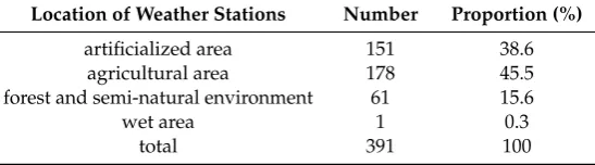
Most of the selected weather stations are located either in artificialized zones, or in agricultural zones (Table1). More precisely, the proportion of weather stations in the agricultural zone is 45.5% (which represents 178 stations) and 38.6% for weather stations located in artificialized zones (151 stations).

Table 1.Location of weather stations studied depending on the type of Land Use Land Cover (LULC).

Location of Weather Stations Number Proportion (%)

artificialized area 151 38.6

agricultural area 178 45.5

forest and semi-natural environment 61 15.6

wet area 1 0.3

total 391 100

(3)

Urban Sci. 2019, 3, x FOR PEER REVIEW 3 of 22

Figure 1. Méteo-France network used and land use on the right-of-way of Landsat 196-28 and 197-28 tiles (data: Météo-France [30] and Corine Land Cover, 2012 [31]).

In addition, the study days must have a cloud cover less than or equal to 10% to present quality remote sensing data. As a result, for this study, six measurement days have been retained during the year 2013, over a period of six months (April to September) and two different seasons (spring and summer): 25 April, 14 July, 21 July, 15 August the 22 August and 23 September (Table 2).

Table 2. Meteorological parameters of study days at the Lyon-Bron station at 12:00 p.m. (data: Météo-France [30]).

Date Temperature (°C) Humidity (%) Rain (mm/h) Wind Average (km/h) Pressure (hPa) Cloud Cover (%)

25 April 2013 21.3 47 0 4 1024.5 1.63

14 July 2013 24.5 52 0 14 1019.5 1.8

21 July 2013 29.4 45 0 6 1016.7 1.96

15 August 2013 21.2 51 0 7 1021.4 0.56

22 August 2013 24.4 44 0 4 1016.8 0.04

23 September

2013 17.8 71 0 4 1024 10.01

Mean 23.1 51.7 0 6.5 1020.5 2.7

Standard

deviation 4.0 10.0 0 3.9 3.4 3.7

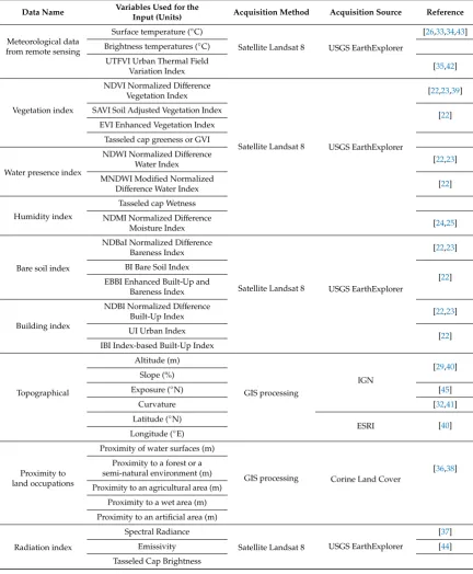
2.2. Twenty-Eight Explanatory Variables Selected from the Literature

Twenty-eight explanatory variables are used to estimate the air temperature over the study area. They have been selected from the literature [22–26,29,32–45]. The variables belong to various categories and can directly be obtained from the supplying organizations or produced by geomatics or remote sensing (Table 3). The remote sensing data is from the United States Geological Survey Figure 1.Méteo-France network used and land use on the right-of-way of Landsat 196-28 and 197-28 tiles (data: Météo-France [30] and Corine Land Cover, 2012 [31]).

Table 2.Meteorological parameters of study days at the Lyon-Bron station at 12:00 p.m. (data: Météo-France [30]).

Date Temperature

(◦C)

Humidity (%)

Rain (mm/h)

Wind Average (km/h)

Pressure (hPa)

Cloud Cover (%)

25 April 2013 21.3 47 0 4 1024.5 1.63

14 July 2013 24.5 52 0 14 1019.5 1.8

21 July 2013 29.4 45 0 6 1016.7 1.96

15 August 2013 21.2 51 0 7 1021.4 0.56

22 August 2013 24.4 44 0 4 1016.8 0.04

23 September 2013 17.8 71 0 4 1024 10.01

Mean 23.1 51.7 0 6.5 1020.5 2.7

Standard deviation 4.0 10.0 0 3.9 3.4 3.7

2.2. Twenty-Eight Explanatory Variables Selected from the Literature

(4)

the biophysical occupation of the land. Thus, at the first level, used in this study, this classification is structured around 5 different levels, namely artificial territories, agricultural territories, forests and semi-natural environments, wetlands (such as marshes or peatlands) and water areas (such as rivers or water bodies).

Table 3.List of explanatory variables selected to estimate fine-scale air temperature.

Data Name Variables Used for the

Input (Units) Acquisition Method Acquisition Source Reference

Meteorological data from remote sensing

Surface temperature (◦C)

Satellite Landsat 8 USGS EarthExplorer

[26,33,34,43] Brightness temperatures (◦C)

UTFVI Urban Thermal Field

Variation Index [35,42]

Vegetation index

NDVI Normalized Difference Vegetation Index

[22,23,39]

SAVI Soil Adjusted Vegetation Index

[22] EVI Enhanced Vegetation Index

Tasseled cap greeness or GVI

Water presence index

NDWI Normalized Difference

Water Index [22,23]

MNDWI Modified Normalized

Difference Water Index [22]

Humidity index

Tasseled cap Wetness NDMI Normalized Difference

Moisture Index [24,25]

Bare soil index

NDBaI Normalized Difference Bareness Index

[22,23]

BI Bare Soil Index

[22] EBBI Enhanced Built-Up and

Bareness Index

Building index

NDBI Normalized Difference

Built-Up Index [22,23]

UI Urban Index

[22] IBI Index-based Built-Up Index

Topographical

Altitude (m)

GIS processing

IGN

[29,40] Slope (%)

Exposure (◦N) [45]

Curvature [32,41]

Latitude (◦

N)

ESRI [40]

Longitude (◦

E)

Proximity to land occupations

Proximity of water surfaces (m)

GIS processing Corine Land Cover

[36,38] Proximity to a forest or a

semi-natural environment (m) Proximity to an agricultural area (m)

Proximity to a wet area (m) Proximity to an artificial area (m)

Radiation index

Spectral Radiance

[37]

Emissivity [44]

Tasseled Cap Brightness

(5)

remaining explanatory variables by integrating a stepwise sorting algorithm which consists of selecting the variables according to their respective contributions to the model. This selection of the model was chosen after having made a sensitivity analysis also on the ascending and descending model. Other statistical regressions were considered, such as the Lasso regression. It has the advantage of selecting only certain explanatory variables in the presence of collinearity. However, Lasso regression is usable only when the number of predictors is greater than the number of observations [49,50]. However, in this study, the number of observations is much higher than the number of predictors. For example, the day of 15 August 2013 includes 112 observations for 28 predictor variables. The number of these stays the same for all of the days.

Moreover, a cross validation is still performed due to its ability to detect over fitting of multiple regression, although multiple regression provides internal validation and randomization [51,52]. In this way, the cross validation presents a more conservative estimate of predictive power. To perform this cross validation, the data have been randomly split each into ‘training’ and ‘testing’ tables consisting of 80% of the data and 20% of the data, respectively. The normality of the residues was verified by analyzing them with the Shapiro–Wilk [47] normality test. The independence of the residues was also checked using the Durbin–Watson test [53].

In order to study the contribution of the explanatory variables not only on a global scale but also in function of the type of LULC, the air temperature modelling have also been made into three zones, depending on the location of the meteorological stations (artificial areas, agricultural areas and forest or semi-natural areas). The modelling has not been carried out over the wet areas and water areas because not enough stations were available.

2.3. A Sensitivity Analysis to Measure the Contribution of Remote Sensing Variables to Air Temperature Estimation

In addition, in order to study the contribution of adding variables from remote sensing data, a sensitivity analysis is performed based on different sets of explanatory variables. Indeed, 6 models with different data sets are performed:

• _{air temperature modelling with all variables,}

• _{air temperature modelling with only remote sensing variables,} • _{air temperature modelling without remote sensing variables,}

• _{air temperature modelling with remote sensing variables but without surface temperature,} • _{air temperature modelling with all variables except surface temperature,}

• _{simple linear regression between air temperature and surface temperature.}

2.4. Location of the Underestimation or Overestimation of Air Temperature Modelling Compared to In Situ Measurements at Météo France’s Weather Stations

The first part of this section is dedicated to the quantification of the underestimation or overestimation of the air temperature model using relative difference. Then, in a second step, these errors are spatialized using LISA and Getis Ord Gi*.

2.4.1. Quantifying the Underestimation or Overestimation of Air Temperatures through a Statistical Model

The variables retained in the multiple linear regressions make it possible to establish a statistical model for estimating air temperatures for a specific day. However, this model may contain estimation errors. These errors can be either a negative difference (model underestimation) or a positive difference (overestimation). This relative difference is given as a percentage and is calculated from the following Equation (1):

Relative di f f erence= (in situ measurments − estimated air temperature)

(6)

2.4.2. Geographical Identification of Statistically Similar Zones: The Use of LISA and Getis Ord Gi* The spatial autocorrelation of the difference between the modelled air temperature and the air temperature measured at the Météo France weather station is determined, on one hand, by using the local spatial association indicator (Anselin Local Moran I-LISA [54]), and, on the other hand, thanks to the degree of grouping of high and low intensity values by the Getis Ord General G [55,56].

LISA makes it possible to group, for statistically significant results (p<0.05), the similarity of a spatial unit with its neighbours. It is calculated from Equation (2):

Li = xi −_x

S2 i

Xn

j =1j,i Wi j

xj−x

, (2)

wherexiis the value of a variable given in pointi,xis the average of this attribute,Wi,jis the weight (coefficient) applied to the comparison between the two locationsiandj, andnis the total number of observations. In addition,S2

iis calculated by the following Equation (3):

S2i= Pn

j =1j,i

xj−x 2

n−₁ . (3)

This technique makes it possible to identify spatial aggregates of features with high or low values as well as outlier spatial points. A cartographic representation showing a cluster type for each statistically significant entity is obtained. Thus, a geographic information system (GIS) allows for distinguishing between a statistically significant cluster of high values (HH), a cluster of low values (LL), an outlier in which a high value is surrounded mainly by low values (HL) and an outlier in which a low value is surrounded mainly by high values (LH).

The local application of the General G statistic is the Getis Ord Gi* statistic [55]. It is used to identify statistically significant spatial clusters (p<0.05) of high and low intensity. Thus, for positive Z scores, the higher they are, the stronger the group of high intensity values is (error overestimating air temperature). On the other hand, the lower the negative Z scores are, the higher the group of low intensity values is (error underestimating air temperature). The Getis Ord Gi* is calculated from Equation (4) below:

G∗_i = Pn

j =1Wi jxj−xPnj =1Wi j s

r nPn

j=1W2i j−

_P_n

j=1Wi j

2

n−₁

, (4)

wherexiis the value of a variable given in pointi,xis the average of this attribute,Wi,jis the weight (coefficient) applied to the comparison between the two locationsiandj, andnis the total number of observations. The mathematical formula for the meanxis presented below (Equation (5)), as well as that of the S, present in the denominator of the Gi* formula (Equation (6)):

x|₌ Pn

j =1xi

n , (5)

S= s

Pn j =1x2i

n −(x)

2

. (6)

3. Results for the Year 2013

(7)

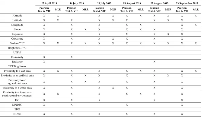
multiple linear regressions, the number of explanatory variables retained decreases further and varies between 6 (15 and 22 August) and 4 (14 July).

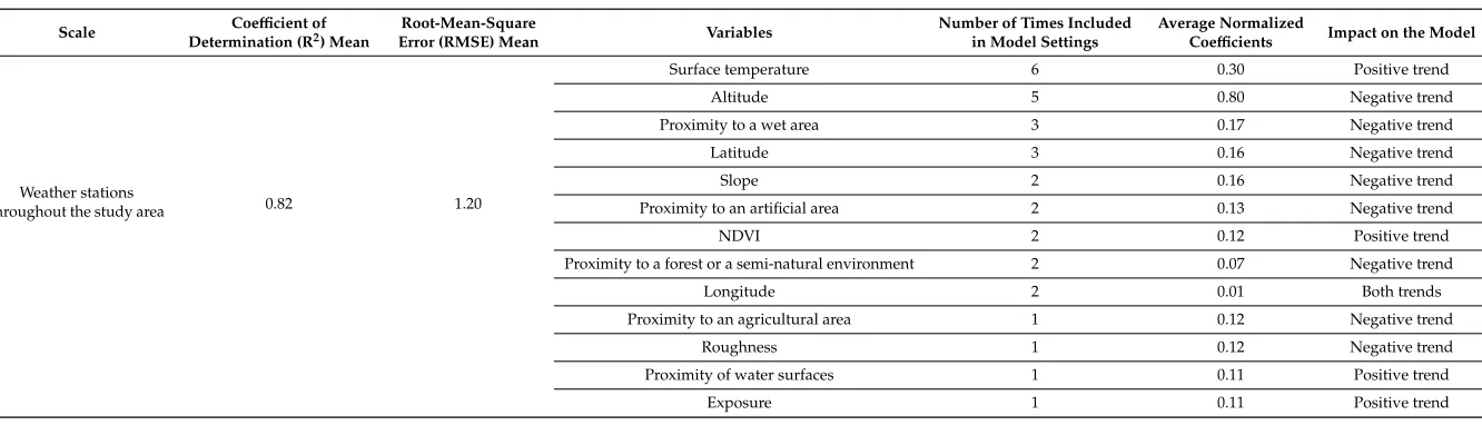
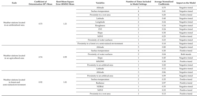
For the whole area, the mean R2is 0.82 when modeling air temperature. A low root mean square error (RMSE) value of 1.20◦C is associated with this high coefficient of determination. These high R2and RMSE are also present when considering the different LULC: for example, the modeling of air temperature based on stations located in a forest or semi-natural environment has a coefficient of determination (R2) of 0.92, with an RMSE of 1.01◦C (Table5).

Altitude and surface temperature variables are the most recurrent and have one of the highest coefficients for each model. Indeed, the altitude is selected five times on the six days for the whole area, the artificialized area and the agricultural area and three times for the forest and semi-natural environment. Surface temperature is selected in each case for the whole area, four times for the artificialized area, four times on the agricultural area and two times for the forest and semi-natural environment. Thus, these two variables represent the key elements for air temperature modeling.

(8)

Table 4.Variables retained (shown by the crosses) after statistical tests (Pearson test and Variance Inflation Factor (VIF)) and multiple linear regression (MLR) for each day studied.

25 April 2013 14 July 2013 21 July 2013 15 August 2013 22 August 2013 23 September 2013

Pearson

Test & VIF MLR

Pearson

Altitude X X X X X X X X X X

Latitude X X X X X X X X X

Longitude X X X X X X X

Slope X X X X X X X X

Exposure X X X X X X X

Curvature X X X X X X X

Surface T◦C X X X X X X X X X X X X

Brightness T◦C

UTFVI

Emissivity X X

Radiance X X

TCT Brightness

Proximity to a wet area X X X X X X X X X

Proximity to an artificial area X X X X X X X X

Proximity to an

agricultural area X X X X X X X

Proximity to a water area X X X X X X X

Proximity to a forest or a

semi-natural environment X X X X X X X X

EVI X X X X X

MNDWI X X X X

EBBI

(9)

Table 4.Cont.

25 April 2013 14 July 2013 21 July 2013 15 August 2013 22 August 2013 23 September 2013

Pearson

NDBI X X

UI

IBI

NDWI X

NDVI X X X X X X X X

SAVI

GVI

NDMI X X X

TCT Wetness

Retained variables (/28) 19 5 17 4 15 5 16 6 16 6 16 5

Table 5.Set of explanatory variables retained by multiple linear regressions for the year 2013.

Scale Coefficient of

Determination (R2_{) Mean}

Root-Mean-Square

Error (RMSE) Mean Variables

Number of Times Included in Model Settings

Average Normalized

Coefficients Impact on the Model

Weather stations

throughout the study area 0.82 1.20

Surface temperature 6 0.30 Positive trend

Altitude 5 0.80 Negative trend

Proximity to a wet area 3 0.17 Negative trend

Latitude 3 0.16 Negative trend

Slope 2 0.16 Negative trend

Proximity to an artificial area 2 0.13 Negative trend

NDVI 2 0.12 Positive trend

Proximity to a forest or a semi-natural environment 2 0.07 Negative trend

Longitude 2 0.01 Both trends

Proximity to an agricultural area 1 0.12 Negative trend

Roughness 1 0.12 Negative trend

Proximity of water surfaces 1 0.11 Positive trend

(10)

Table 5.Cont.

Scale Coefficient of

Determination (R2) Mean

Root-Mean-Square

Error (RMSE) Mean Variables

Number of Times Included in Model Settings

Average Normalized

Coefficients Impact on the Model

Weather stations located

in an artificialized area 0.73 1.21

Surface temperature 4 0.41 Negative trend

Proximity to a wet area 4 0.28 Positive trend

Longitude 2 0.24 Negative trend

Roughness 2 0.24 Negative trend

EVI 2 0.24 Negative trend

Proximity of water surfaces 1 0.23 Negative trend

Proximity to a forest or a semi-natural environment 1 0.10 Negative trend

Weather stations located

in an agricultural area 0.74 0.95

Proximity of water surfaces 2 0.04 Both trends

MNDWI 1 0.30 Positive trend

Weather stations located in forest and semi-natural environment

0.92 1.01

Radiance 1 0.97 Positive trend

NDBAI 1 0.35 Negative trend

(11)

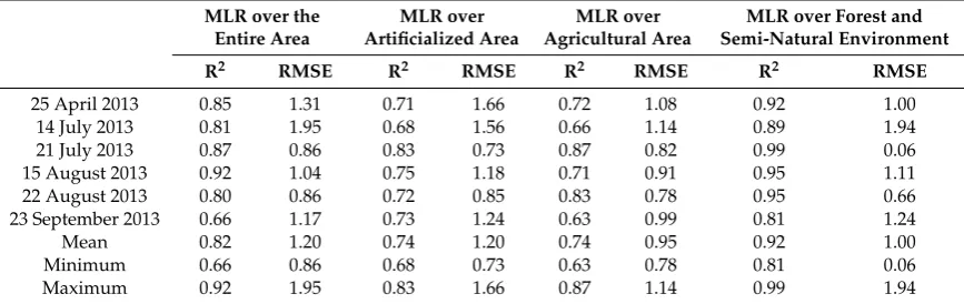
Table 6.Part of the variance explained in the modeling of air temperature over the entire study area and by land cover.

MLR over the Entire Area

MLR over Artificialized Area

MLR over Agricultural Area

MLR over Forest and Semi-Natural Environment

R2 RMSE R2 RMSE R2 RMSE R2 RMSE

25 April 2013 0.85 1.31 0.71 1.66 0.72 1.08 0.92 1.00

14 July 2013 0.81 1.95 0.68 1.56 0.66 1.14 0.89 1.94

21 July 2013 0.87 0.86 0.83 0.73 0.87 0.82 0.99 0.06

15 August 2013 0.92 1.04 0.75 1.18 0.71 0.91 0.95 1.11

22 August 2013 0.80 0.86 0.72 0.85 0.83 0.78 0.95 0.66

23 September 2013 0.66 1.17 0.73 1.24 0.63 0.99 0.81 1.24

Mean 0.82 1.20 0.74 1.20 0.74 0.95 0.92 1.00

Minimum 0.66 0.86 0.68 0.73 0.63 0.78 0.81 0.06

Maximum 0.92 1.95 0.83 1.66 0.87 1.14 0.99 1.94

The coefficients obtained for each day and each LULC, from the multiple linear regressions, allow for modeling the air temperature at any point of the study area. For example, when focusing on the entire study area, the following equations are obtained (Equations (7)–(12)), allowing for obtaining the modelled air temperature maps (Figure2):

- for 25 April:

Air temperature=57.0− _5.1−3×_Altitude−_0.8×_Latitude₊_0.2×

Sur f ace temperature+2.9−5×_{Distance to a wet area}−_5.7−₄_×

Distance to f orest, (7) - for 14 July:

Air temperature=13.0+0.4×_{Sur f ace temperature}−_4.7−4×

Distance to an arti f icial area−_4.0−4×_{Distance to an agricol area}−_0.1×_Slope_, (8) - for 21 July:

Air temperature=49.3−_7.2−3×_Altitude−_0.5×_Latitude₊_0.1×

Sur f ace temperature+4.3−5×_{Distance to water sur f ace}−_4.1×_Curvature_, (9) - for 15 August:

Air temperature=16.1−_5.2−₃_×

Altitude+0.9×_Longitude₊_0.1×_{Sur f ace temperature}

+3.5−5×_{Distance to a wet area}− _4.0−4×_{Distance to a f orest}−_5.4−2×_Slope_, (10) - for 22 August:

Air temperature=74.1−_5.3−₃_×

Altitude−_1.1×_Latitude₊_8.5−₂_×

Sur f ace temperature+1.0×_NDVI−_1.5−4×_{Distance to an arti f icial area}₊ _2.0−3×_Exposition_, (11) - for 23 September:

Air temperature=19.0−_5.6−3×_Altitude−_0.5×_Longitude+2.9×_NDVI+

(12)

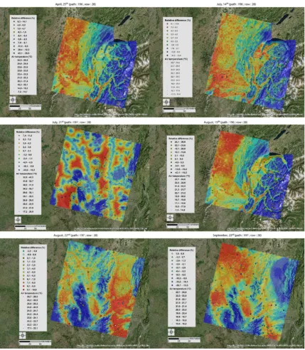
According to Figure2, general trends are emerging. On the days when Landsat 8 passes over path 196 and row 28 (25 April, 14 July and 15 August), a heat corridor from northwest to southwest can be observed. This zone includes the Metropolitan Area of Lyon to the southwest where air temperatures are about 10◦C higher than the lowest temperatures located to the east in the Alps and in the centre of the Haut Jura Regional Nature Reserve.

Urban Sci. 2019, 3, x FOR PEER REVIEW 12 of 22

Figure 2. Estimated air temperature for all days studied with relative difference between the modelling and the in situ measurements (quantile discretization).

4. Discussion

4.1. Characterization of Error Location and Intensity

From the coefficients of determination obtained by the multiple linear regressions for each day (Table 5), the statistical model achieves model air temperatures in a satisfactory way, more precisely

with an R2_{average of 0.82 for the entire study area. However, there are prediction errors that need to}

be quantified and located.

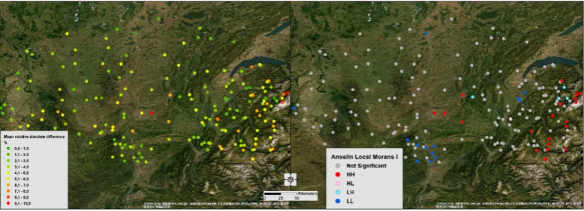
For the first time, averages of the absolute relative differences between the in situ and modelled air temperatures measurements for the six days have been located in the study area (Figure 3—left). For the second time, the spatial clustering of the statistically close relative differences values (LISA) have been identified (Figure 3—right).

Figure 2.Estimated air temperature for all days studied with relative difference between the modelling and the in situ measurements (quantile discretization).

During the days when the satellite orbits on path 196 and row 28 (21 July, 22 August and 23 September), the air temperature remains high over the Lyon Metropolis (southeast) but also around Clermont Ferrand (centre west) with a difference of+5◦

(13)

However, with all estimates, there is a certain percentage of error highlighted by the relative difference between the Meteo France weather stations and the air temperature model by multiple linear regression (Equation (1)). This relative difference fluctuates day by day, between an underestimation or overestimation for the same station (2.9% for the 15 August and 1.4% for the 22 August compared to the data from the Lyon Saint Exupéry’s weather station) and with more or less significant differences (1.7% for the 25 April to 19.3% for the 14 July compared to the Feclaz’s weather station located in the centre east of the study area). These estimation errors are studied in the discussion part.

4. Discussion

4.1. Characterization of Error Location and Intensity

From the coefficients of determination obtained by the multiple linear regressions for each day (Table5), the statistical model achieves model air temperatures in a satisfactory way, more precisely with an R2average of 0.82 for the entire study area. However, there are prediction errors that need to be quantified and located.

For the first time, averages of the absolute relative differences between the in situ and modelled air temperatures measurements for the six days have been located in the study area (Figure3—left). For the second time, the spatial clustering of the statistically close relative differences values (LISA) have been identified (Figure_{Urban Sci.}_2019,₃_{, x FOR PEER REVIEW}3—right). _{13 of 22}

Figure 3. Averages of the absolute relative differences for the six days (left) and spatial clustering of the statistically close relative differences values (LISA—right).

Thus, a clustering of very low errors (LL) is observed in the south of the city of Lyon (south central on the map). This error fluctuates from a minimum of 1% to a maximum of 1.8% on these different measurement points. On the other hand, two zones have important errors (HH) in estimating air temperature. The first is located in the centre of the study area and concentrates in particular on the two main weather stations of Lyon (Lyon Bron and Lyon Saint Exupéry), with an average of the absolute relative differences ranging from 5.3% to 9.2%. The second area is located to the east of the study area, in the Alps, with an average of absolute relative differences ranging from 5.7% to 9.0%. These two areas with high errors in air temperature modelling have particular spatial configurations, which may explain these important differences. The first area is a dense urban space, where other prediction variables must be included, such as the sky view factor [57–59] or anthropogenic heat [60]. The second is a mountain area where the Alpine arc acts in response to particular climatic variations.

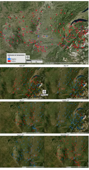
The prediction errors are located in a global way for all days (Figure 4). However, the average obtained hides the variations over each day, notably since the satellite approaches were found to underestimate measured turbulent heat fluxes and anthropogenic fluxes [61]. Moreover, temperature is one of the variables used in climate modelling. However, the latter is not a stationary phenomenon [26,52]. In this study, the prediction of air temperature gives results that are statistically very close to the air temperature measured at professional meteorological stations (R2 average of 0.82 over the entire study area). However, errors still do exist. Since these errors depend on the modelling of a non-stationary phenomenon, they also vary over time. Thus, they depend on the climate and the synoptic weather pattern of the day studied but also on previous days, also influencing variables from remote sensing such as MNDWI or NDMI. Indeed, for several days, the relative error may not be constant, being positive for one day and negative for another (Figure 5). Similarly, the magnitude of the error is not necessarily constant. Consequently, the clusters of negative or positive errors have been studied using the LISA model.

For the days of 25 April, 14 July and 15 August, a typical and recurrent spatial distribution of estimation errors can be observed, both in the LISA analysis (Figure 5) and in the Gi* analysis (Figure 6). Indeed, the model tends to underestimate the measurements in an area south of Lake Geneva, with LL type clusters (Figure 5) or negative z score with very low values (Figure 6). Conversely, an overestimated HH cluster is found in the Alpine massif. This overestimation cluster is also found in the Gi* results with stations with statistically significant high positive z score values. In contrast to these marked configurations, the days of 21 July, 22 August and 23 September do not seem to clearly show recurrent clusters of overestimation or underestimation, either with the LISA (Figure 5) or Gi* technique (Figure 6). Indeed, there is very little clustering of statistically significant station errors. For example, only three stations form an HH cluster on 21 July and none on 23 September (Figure 5). This may be explained in particular by a different study area footprint with a less accentuated relief and less marked topoclimatic effects.

Figure 3.Averages of the absolute relative differences for the six days (left) and spatial clustering of the statistically close relative differences values (LISA—right).

Thus, a clustering of very low errors (LL) is observed in the south of the city of Lyon (south central on the map). This error fluctuates from a minimum of 1% to a maximum of 1.8% on these different measurement points. On the other hand, two zones have important errors (HH) in estimating air temperature. The first is located in the centre of the study area and concentrates in particular on the two main weather stations of Lyon (Lyon Bron and Lyon Saint Exupéry), with an average of the absolute relative differences ranging from 5.3% to 9.2%. The second area is located to the east of the study area, in the Alps, with an average of absolute relative differences ranging from 5.7% to 9.0%. These two areas with high errors in air temperature modelling have particular spatial configurations, which may explain these important differences. The first area is a dense urban space, where other prediction variables must be included, such as the sky view factor [57–59] or anthropogenic heat [60]. The second is a mountain area where the Alpine arc acts in response to particular climatic variations.

(14)

very close to the air temperature measured at professional meteorological stations (R2average of 0.82 over the entire study area). However, errors still do exist. Since these errors depend on the modelling of a non-stationary phenomenon, they also vary over time. Thus, they depend on the climate and the synoptic weather pattern of the day studied but also on previous days, also influencing variables from remote sensing such as MNDWI or NDMI. Indeed, for several days, the relative error may not be constant, being positive for one day and negative for another (Figure5). Similarly, the magnitude of the error is not necessarily constant. Consequently, the clusters of negative or positive errors have been studied using the LISA model.

For the days of 25 April, 14 July and 15 August, a typical and recurrent spatial distribution of estimation errors can be observed, both in the LISA analysis (Figure5) and in the Gi* analysis (Figure6). Indeed, the model tends to underestimate the measurements in an area south of Lake Geneva, with LL type clusters (Figure5) or negative z score with very low values (Figure6). Conversely, an overestimated HH cluster is found in the Alpine massif. This overestimation cluster is also found in the Gi* results with stations with statistically significant high positive z score values.

In contrast to these marked configurations, the days of 21 July, 22 August and 23 September do not seem to clearly show recurrent clusters of overestimation or underestimation, either with the LISA (Figure5) or Gi* technique (Figure6). Indeed, there is very little clustering of statistically significant station errors. For example, only three stations form an HH cluster on 21 July and none on 23 September (Figure5). This may be explained in particular by a different study area footprint with a

(15)

Figure 4. Pie charts of the number of times the relative error of air temperature estimation (positive or negative) for the six days studied (top figure) and detailed day by day (bottom figures).

(16)

Figure 5. LISA of the relative differences between in situ and modelled air temperatures for each day studied.

(17)

Figure 6. Getis Ord GI* of the relative differences between in situ and modelled air temperatures for each day studied.

4.2. The Contribution of Remote Sensing Variables to the Quality of the Air Temperature Prediction Model

A sensitivity analysis was conducted to estimate the contribution of variables from remote sensing products (Section 2.3). As presented in the previous section, air temperature modelling with all variables gives very satisfactory results (in red in Figure 7). For example, for the day of 25 April, the determination coefficient is 0.85 and the RMSE is 1.31 °C.

Figure 6.Getis Ord GI* of the relative differences between in situ and modelled air temperatures for each day studied.

4.2. The Contribution of Remote Sensing Variables to the Quality of the Air Temperature Prediction Model A sensitivity analysis was conducted to estimate the contribution of variables from remote sensing products (Section 2.3). As presented in the previous section, air temperature modelling with all variables gives very satisfactory results (in red in Figure7). For example, for the day of 25 April, the determination coefficient is 0.85 and the RMSE is 1.31◦

(18)

Figure 7. Results of the different modelling of air temperature over the entire study area: R2_{on the}

left axis; Root-Mean-Square Error (RMSE) on the right axis).

When considering modelling results based only on classical air modelling variables (topography, land use, etc.), i.e., without the variables from remote sensing, it can be seen that the results are still correct (in blue in Figure 7) but lower than the previous ones. For example, for the day of 25 April, the determination coefficient is 0.76 and the RMSE is 1.62 °C.

Conversely, air temperature modelling carried out only with variables from remote sensing products (grey in Figure 7) is even less efficient. The day of 25 April 2013 has an R2_{of 0.68 and an} RMSE of 1.86 °C. This is not surprising because the previous results (Section 3, Table 4) indicated that the dominant variable is the elevation, both in terms of the number of times this variable has been included in the model and in terms of its normalized coefficient.

These same results indicate that the second most important variable contributing to the model is surface temperature. This is clearly shown in Figure 7 when looking at the results of modelling with all variables except surface temperature (green in Figure 7). The results of this modeling are thus positioned between those obtained with all variables and those obtained with conventional variables. Therefore, for the day of 25 April, the determination coefficient is 0.78 and the RMSE is 1.55 °C. This confirms the interest of integrating surface temperature into air temperature modelling, as previous studies have also suggested [19–21].

However, this relationship between air and surface temperatures is not constant and varies according to atmospheric conditions, among other things. Indeed, for the days of 25 April or 14 July 2013, the relationship between these two variables is relatively strong, with R2_{s of 0.64 and 0.67} respectively (in yellow in Figure 8). Conversely, this relationship may be weaker, as for the days of 22 August or 23 September 2013, with R2_{s of 0.28 and 0.20, respectively.}

In addition, surface temperature is not the only interesting variable from remote sensing that is integrated into the modelling. When considering modelling with remotely sensed variables, with the exception of surface temperature, the results obtained are not insignificant (in purple in Figure 7). Indeed, for example, the R2_{is 0.37 for the day of 25 April and 0.49 for the day of 14 July 2013. This} also confirms the value of not only adding surface temperature to remote sensing products, but also other complementary variables such as spectral indices. This is one of the major contributions of this study. Indeed, the NDVI is used twice in the models for the entire study area and once in the models for artificialized areas and forest and semi-natural environment (Table 4). The EVI, MNDWI and NDBaI are also used in some models, especially with relatively high standardized coefficients (e.g.,

Figure 7.Results of the different modelling of air temperature over the entire study area: R2on the left axis; Root-Mean-Square Error (RMSE) on the right axis).

When considering modelling results based only on classical air modelling variables (topography, land use, etc.), i.e., without the variables from remote sensing, it can be seen that the results are still correct (in blue in Figure7) but lower than the previous ones. For example, for the day of 25 April, the determination coefficient is 0.76 and the RMSE is 1.62◦

C.

Conversely, air temperature modelling carried out only with variables from remote sensing products (grey in Figure7) is even less efficient. The day of 25 April 2013 has an R2of 0.68 and an RMSE of 1.86◦C. This is not surprising because the previous results (Section3, Table4) indicated that the dominant variable is the elevation, both in terms of the number of times this variable has been included in the model and in terms of its normalized coefficient.

These same results indicate that the second most important variable contributing to the model is surface temperature. This is clearly shown in Figure7when looking at the results of modelling with all variables except surface temperature (green in Figure7). The results of this modeling are thus positioned between those obtained with all variables and those obtained with conventional variables. Therefore, for the day of 25 April, the determination coefficient is 0.78 and the RMSE is 1.55◦C. This confirms the interest of integrating surface temperature into air temperature modelling, as previous studies have also suggested [19–21].

However, this relationship between air and surface temperatures is not constant and varies according to atmospheric conditions, among other things. Indeed, for the days of 25 April or 14 July 2013, the relationship between these two variables is relatively strong, with R2s of 0.64 and 0.67 respectively (in yellow in Figure7). Conversely, this relationship may be weaker, as for the days of 22 August or 23 September 2013, with R2s of 0.28 and 0.20, respectively.

(19)

0.30 for MNDWI for modelling in agricultural areas and 0.35 for NDBaI for forest and semi-natural environment).

4.3. Limits and Outlooks

Several limits can be considered. The first concerns the availability of the data. Indeed, the Landsat satellite passes only every 16 days over the same area which reduces the number of scenes possible. In addition, clouds have to be present. The presence of clouds would distort the modeling of the air temperature since the model integrates the surface temperature. Indeed, a cloud surface temperature is mostly negative, which is not the case of the ground under these clouds. Finally, as the last limits to this study, it can be noted that the research was carried out only on one year, 2013, with only six days available due to the dependence of valid data on the presence of clouds.

The second limit relates to the necessity to have one model equation per day due to non-stationary weather conditions [52]. These limits can be at the same time a perspective of work, while continuing the study on several years to validate the contribution of the remote sensing variables in the air temperature model.

For other perspectives, some other data satellites may be used. For example, the use of the Sentinel 2 satellite with 10 m resolution may help to increase the model by the remote sensing variables. In addition, multiple linear regressions have been used to model air temperature. However, this model does not consider the spatial variability of the data. Thus, modeling air temperature by geographically weighted regression can probe the spatial heterogeneity in data relationships [12,62].

5. Conclusions

The knowledge of air temperature distribution mechanisms is a key element in many areas, particularly in the context of urban adaptation to climate change and heat waves. In the context of this study, the modelling of air temperature by multiple linear regression gives very satisfying results for all these study days over the year 2013 (mean R2of 0.82). The average of the absolute relative differences between the modelled air temperatures and those measured by the Météo France weather stations over all day ranges from 0.47% to 10.2%.

However, there are episodic variations in these estimates of air temperature and the associated prediction errors. This is why the use of LISA and Getis Ord GI* statistics makes it possible to quickly localise statically similar values and to be able to analyse differences and similarities on a day by day basis. Thus, there are hot spot errors in the Alps and cold spot errors close to Lake Geneva.

The contribution of remote sensing variables in the air temperature prediction model is a real added value since this integration allows us to gain in quality both an increase in the determination coefficient (a 12% benefit from the variance on average) and a decrease in the RMSE (an accuracy of more than 0.7◦C on average).

Finally, and given the current policy of streamlining the observation sites of the Météo France network, this methodology could be of some use for the weakly instrumented territories. Thus, the methods described in this study are reproducible for any area and do not require any specific resources, except the access to explanatory variables and source dataset. It can be highly useful in many fields as urban studies for heat stress planning. However, air temperature modelling will not replace direct field measurements. Thus, if cities wish to know the urban thermal gradients precisely, this necessarily requires the implementation of a dense ground measurement network.

Author Contributions:Conceptualization, L.A. and F.R.; methodology, L.A. and F.R.; validation, L.A. and F.R.; formal analysis, L.A. and F.R.; writing—original draft preparation, L.A. and F.R.; writing—review and editing, L.A. and F.R.; supervision, L.A. and F.R.; project administration, L.A. and F.R.

Funding:This research received no external funding.

(20)

Conflicts of Interest:The authors declare no conflict of interest.

References

1. Jouzel, J. Le Climat de la France au XXIe Siècle—Volume 4—Scénarios Régionalisés: Publishing in 2014 for Metropolitan France and Overseas Regions. 2014. Available online:http://www.ladocumentationfrancaise. fr/rapports-publics/144000543/index.shtml(accessed on 19 April 2019).

2. Météo-France.Changement Climatique en Rhône-Alpes; Météo-France: Bron, France, 2011.

3. ORECC.Fiche Indicateur—Climat: Changement Climatique en Auvergne Rhône-Alpes—Températures Moyennes Annuelles et Saisonnières; ORECC: Lyon, France, 2017; Available online: http://orecc.auvergnerhonealpes. fr/fileadmin/user_upload/mediatheque/orecc/Documents/Donnees_territoriales/Indicateurs/ORECC_ FicheIndicateur_2017_V20170929_CumulPrecipitations.pdf(accessed on 20 September 2019).

4. Keeratikasikorn, C.; Bonafoni, S. Urban Heat Island Analysis over the Land Use Zoning Plan of Bangkok by Means of Landsat 8 Imagery.Remote Sens.2018,10, 440. [CrossRef]

5. Fallmann, J.; Forkel, R.; Emeis, S. Secondary effects of urban heat island mitigation measures on air quality.

Atmos. Environ.2016,125, 199–211. [CrossRef]

6. Benas, N.; Chrysoulakis, N.; Cartalis, C. Trends of urban surface temperature and heat island characteristics in the Mediterranean.Theor. Appl. Climatol.2017,130, 807–816. [CrossRef]

7. Heino, R. Urban effect on climatic elements in Finland.Geophysica1978,15, 171–188.

8. Giguère, M.; National Institute of Public Health of Québec, Environmental and Occupational Biological Risks Directorate.Mesures de Lutte aux Îlots de Chaleur Urbains Revue de Littérature; Environmental and Occupational Biological Risks Directorate, I National Institute of Public Health of Québec: Québec, QC, Canada, 2010. 9. Wang, M.; He, G.; Zhang, Z.; Wang, G.; Zhang, Z.; Cao, X.; Wu, Z.; Liu, X. Comparison of Spatial Interpolation

and Regression Analysis Models for an Estimation of Monthly near Surface Air Temperature in China.

Remote Sens.2017,9, 1278. [CrossRef]

10. Zhang, Z.; Du, Q. A Bayesian Kriging Regression Method to Estimate Air Temperature Using Remote Sensing Data.Remote Sens.2019,11, 767. [CrossRef]

11. Chen, Y.; Quan, J.; Zhan, W.; Guo, Z. Enhanced Statistical Estimation of Air Temperature Incorporating Nighttime Light Data.Remote Sens. 2016,8, 656. [CrossRef]

12. Zhao, C.; Jensen, J.; Weng, Q.; Weaver, R. A Geographically Weighted Regression Analysis of the Underlying Factors Related to the Surface Urban Heat Island Phenomenon.Remote Sens.2018,10, 1428. [CrossRef] 13. Wicki, A.; Parlow, E. Multiple Regression Analysis for Unmixing of Surface Temperature Data in an Urban

Environment.Remote Sens. 2017,9, 684. [CrossRef]

14. Mira, M.; Ninyerola, M.; Batalla, M.; Pesquer, L.; Pons, X. Improving Mean Minimum and Maximum Month-to-Month Air Temperature Surfaces Using Satellite-Derived Land Surface Temperature.Remote Sens.

2017,9, 1313. [CrossRef]

15. Sun, Y.; Gao, C.; Li, J.; Wang, R.; Liu, J. Quantifying the Effects of Urban Form on Land Surface Temperature in Subtropical High-Density Urban Areas Using Machine Learning.Remote Sens.2019,11, 959. [CrossRef] 16. The Senate. Closures of Météo-France Weather Stations and the Future of the French Public Weather

Service—The Senate. Available online: https://www.senat.fr/questions/base/2011/qSEQ110317685.html

(accessed on 25 April 2019).

17. Barroux, R. Météo France’s Forecasts in the Budgetary Crisis. Published 15 December 2014. Available online:https://www.lemonde.fr/planete/article/2014/12/15/ les-previsions-de-meteo-france-dans-la-tourmente-budgetaire_4540743_3244.html(accessed on 25 April 2019).

18. Stewart, I.D. A systematic review and scientific critique of methodology in modern urban heat island literature.Int. J. Climatol.2011,31, 200–217. [CrossRef]

19. Oyler, J.W.; Dobrowski, S.Z.; Holden, Z.A.; Running, S.W. Remotely Sensed Land Skin Temperature as a Spatial Predictor of Air Temperature across the Conterminous United States.J. Appl. Meteorol. Climatol.2016,

55, 1441–1457. [CrossRef]

(21)

21. Hashimoto, H.; Wang, W.; Melton, F.S.; Moreno, A.L.; Ganguly, S.; Michaelis, A.R.; Nemani, R.R. High-resolution mapping of daily climate variables by aggregating multiple spatial data sets with the random forest algorithm over the conterminous United States. Int. J. Climatol. 2019, 39, 2964–2983. [CrossRef]

22. Hasanlou, M.; Mostofi, N. Investigating Urban Heat Island Estimation and Relation between Various Land Cover Indices in Tehran City Using Landsat 8 Imagery. In Proceedings of the 1st International Electronic Conference on Remote Sensing, online, 22 June–5 July 2015.

23. Chen, X.-L.; Zhao, H.-M.; Li, P.-X.; Yin, J. Remote sensing image-based analysis of the relationship between urban heat island and land use/cover changes.Remote Sens. Environ.2006,104, 133–146. [CrossRef] 24. Jin, S.; Sader, S. Comparison of time series Tasseled Cap wetness and the normalized difference moisture

index in detecting forest disturbances.Remote Sens. Environ.2005,94, 364–372. [CrossRef]

25. Nguyen, K.-A.; Liou, Y.-A.; Li, M.-H.; Anh Tran, T. Zoning eco-environmental vulnerability for environmentalmanagement and protection.Ecol. Indic.2016,69. [CrossRef]

26. Tsin, P.K.; Knudby, A.; Krayenhoff, E.S.; Ho, H.C.; Brauer, M.; Henderson, S.B. Microscale mobile monitoring of urban air temperature.Urban Clim.2016,18, 58–72. [CrossRef]

27. Nichol, J.E.; To, P.H. Temporal characteristics of thermal satellite images for urban heat stress and heat island mapping.ISPRS J. Photogramm. Remote Sens.2012,74, 153–162. [CrossRef]

28. Renard, F.; Alonso, L.; Fitts, Y.; Hadjiosif, A.; Comby, J. Evaluation of the Effect of Urban Redevelopment on Surface Urban Heat Islands.Remote Sens. 2019,11, 299. [CrossRef]

29. Kim, Y.-H.; Baik, J.-J. Daily maximum urban heat island intensity in large cities of Korea.Theor. Appl. Climatol.

2004,79, 151–164. [CrossRef]

30. Météo-France. METEO-FRANCE: Publithèque. Available online:https://publitheque.meteo.fr/okapi/accueil/ okapiWebPubli/index.jsp(accessed on 19 September 2019).

31. Corine Land Cover. European Environment Agency. 2012. Available online:https://www.eea.europa.eu/ publications/COR0-landcover(accessed on 19 September 2019).

32. Hafner, J.; Kidder, S.Q. Urban Heat Island Modeling in Conjunction with Satellite-Derived Surface/Soil Parameters.J. Appl. Meteorol.1999,38, 448–465. [CrossRef]

33. Sobrino, J.; Jimenez-Munoz, J.-C.; Paolini, L. Land surface temperature retrieval from LANDSAT TM 5.

Remote Sens. Environ.2004,90, 434–440. [CrossRef]

34. Tran, H.; Uchihama, D.; Ochi, S.; Yasuoka, Y. Assessment with satellite data of the urban heat island effects in Asian mega cities.Int. J. Appl. Earth Obs. Geoinf.2006,8, 34–48. [CrossRef]

35. Liu, L.; Zhang, Y. Urban Heat Island Analysis Using the Landsat TM Data and ASTER Data: A Case Study in Hong Kong.Remote Sens.2011,3, 1535–1552. [CrossRef]

36. Shohei, K.; Takeki, I.; Hideo, T. Relationship between Terra/ASTER Land Surface Temperature and Ground-observed Air Temperature.Geogr. Rev. Jpn. Ser. B2016,88, 38–44. [CrossRef]

37. Iizawa, I.; Umetani, K.; Ito, A.; Yajima, A.; Ono, K.; Amemura, N.; Onishi, M.; Sakai, S. Time evolution of an urban heat island from high-density observations in Kyoto city.Sci. Online Lett. Atmos.2016,12, 51–54. [CrossRef]

38. Madelin, M.; Bigot, S.; Duché, S.; Rome, S. Intensitéet délimitation de l’îlot de chaleur nocturne de surface sur l’agglomération parisienne. In Proceedings of the Colloque International de l’Association Internationale de Climatologie (AIC), Sfax, Tunisia, 3–6 July 2017.

39. Ro¸sca, C.F.; Harpa, G.V.; Croitoru, A.-E.; Herbel, I.; Imbroane, A.M.; Burada, D.C. The impact of climatic and non-climatic factors on land surface temperature in southwestern Romania.Theor. Appl. Climatol.2017,130, 775–790. [CrossRef]

40. Weng, Q.; Firozjaei, M.K.; Sedighi, A.; Kiavarz, M.; Alavipanah, S.K. Statistical analysis of surface urban heat island intensity variations: A case study of Babol city, Iran.GIScience Remote Sens.2019,56, 576–604. [CrossRef]

41. Weng, Q.; Quattrochi, D. Thermal remote sensing of urban areas: An introduction to the special issue.

Remote Sens. Environ.2006,104, 119–122. [CrossRef]

42. Alfraihat, R.; Mulugeta, G.; Gala, T.S. Ecological Evaluation of Urban Heat Island in Chicago City, USA.

(22)

43. Gallo, K.; Hale, R.; Tarpley, D.; Yu, Y. Evaluation of the Relationship between Air and Land Surface Temperature under Clear- and Cloudy-Sky Conditions. J. Appl. Meteorol. Climatol. 2010, 50, 767–775. [CrossRef]

44. Taha, H. Urban climates and heat islands: Albedo, evapotranspiration, and anthropogenic heat.Energy Build.

1997,25, 99–103. [CrossRef]

45. Ali-Toudert, F.; Mayer, H. Effects of asymmetry, galleries, overhanging façades and vegetation on thermal comfort in urban street canyons.Sol. Energy2007,81, 742–754. [CrossRef]

46. Barsi, J.A.; Lee, K.; Kvaran, G.; Markham, B.L.; Pedelty, J.A. The Spectral Response of the Landsat-8 Operational Land Imager.Remote Sens. 2014,6, 10232–10251. [CrossRef]

47. Shapiro, S.S.; Wilk, M.B. An analysis of variance test for normality (complete samples).Biometrika1965,52, 591–611. [CrossRef]

48. OECD. Handbook on Constructing Composite Indicators: Methodology and User Guide. Available online:

http://www.oecd.org/fr/els/soc/handbookonconstructingcompositeindicatorsmethodologyanduserguide. htm(accessed on 17 April 2019).

49. Tibshirani, R. Regression Shrinkage and Selection via the Lasso. J. R. Stat. Soc. Ser. B Methodol. 1996,58, 267–288. [CrossRef]

50. Reid, S.; Tibshirani, R.; Friedman, J. A study of error variance estimation in lasso regression.Stat. Sin.2016,

26, 35–67. [CrossRef]

51. Voelkel, J.; Shandas, V.; Haggerty, B. Developing High-Resolution Descriptions of Urban Heat Islands: A Public Health Imperative.Prev. Chronic Dis.2016,13. [CrossRef]

52. Shandas, V.; Voelkel, J.; Williams, J.; Hoffman, J. Integrating Satellite and Ground Measurements for Predicting Locations of Extreme Urban Heat.Climate2019,7, 5. [CrossRef]

53. Durbin, J.; Watson, G.S. Testing for serial correlation in least squares regression. I.Biometrika1950,37, 409–428. [CrossRef] [PubMed]

54. Anselin, L. Local Indicators of Spatial Association—LISA.Geogr. Anal.1995,27, 93–115. [CrossRef] 55. Getis, A.; Ord, J. A Research Agenda for Geographic Information Science. InSpatial Analysis and Modeling

in a GIS Environment; McMaster, R.B., Usery, E.L., Eds.; CRC Press: Boca Raton, FL, USA, 1996; p. 416. Available online:https://books.google.fr/books?hl=fr&lr=&id=k9x0B3V3op0C&oi=fnd&pg=PA157&ots= cOnYyDRjKL&sig=nW-5WZ7_04hBe-lbgv2MdwBABBM&redir_esc=y#v=onepage&q&f=false(accessed on 3 May 2019).

56. Getis, A.; Ord, J.K. The Analysis of Spatial Association by Use of Distance Statistics.Geogr. Anal.1992,24. [CrossRef]

57. Qaid, A.; Lamit, H.B.; Ossen, D.R.; Rasidi, M.H. Effect of the position of the visible sky in determining the sky view factor on micrometeorological and human thermal comfort conditions in urban street canyons.

Theor. Appl. Climatol.2018,131, 1083–1100. [CrossRef]

58. Chen, L.; Ng, E.; An, X.; Ren, C.; Lee, M.; Wang, U.; He, Z. Sky view factor analysis of street canyons and its implications for daytime intra-urban air temperature differentials in high-rise, high-density urban areas of Hong Kong: A GIS-based simulation approach.Int. J. Climatol.2012,32, 121–136. [CrossRef]

59. Hodul, M.; Knudby, A.; Ho, H.C. Estimation of Continuous Urban Sky View Factor from Landsat Data Using Shadow Detection.Remote Sens.2016,8, 568. [CrossRef]

60. Dong, Y.; Varquez, A.C.G.; Kanda, M. Global anthropogenic heat flux database with high spatial resolution.

Atmos. Environ.2017,150, 276–294. [CrossRef]

61. Chrysoulakis, N.; Grimmond, S.; Feigenwinter, C.; Lindberg, F.; Gastellu-Etchegorry, J.-P.; Marconcini, M.; Mitraka, Z.; Stagakis, S.; Crawford, B.; Olofson, F.; et al. Urban energy exchanges monitoring from space.

Sci. Rep.2018,8, 1–8. [CrossRef]

62. Lin, X.; Su, Y.-C.; Shang, J.; Sha, J.; Li, X.; Sun, Y.-Y.; Ji, J.; Jin, B. Geographically Weighted Regression Effects on Soil Zinc Content Hyperspectral Modeling by Applying the Fractional-Order Differential.Remote Sens.

2019,11, 636. [CrossRef]