A scientific algorithm to simultaneously retrieve carbon monoxide
and methane from TROPOMI onboard Sentinel-5 Precursor
Oliver Schneising1, Michael Buchwitz1, Maximilian Reuter1, Heinrich Bovensmann1, John P. Burrows1, Tobias Borsdorff2, Nicholas M. Deutscher3, Dietrich G. Feist4,5,6, David W. T. Griffith3, Frank Hase7, Christian Hermans8, Laura T. Iraci9, Rigel Kivi10, Jochen Landgraf2, Isamu Morino11, Justus Notholt1, Christof Petri1, David F. Pollard12, Sébastien Roche13, Kei Shiomi14, Kimberly Strong13, Ralf Sussmann15, Voltaire A. Velazco3, Thorsten Warneke1, and Debra Wunch13
1Institute of Environmental Physics (IUP), University of Bremen FB1, Bremen, Germany
2SRON Netherlands Institute for Space Research, Earth Science Group (ESG), Utrecht, the Netherlands
3Centre for Atmospheric Chemistry, School of Earth, Atmosphere and Life Sciences, University of Wollongong, Wollongong, Australia
4Ludwig-Maximilians-Universität München, Lehrstuhl für Physik der Atmosphäre, Munich, Germany
5Deutsches Zentrum für Luft- und Raumfahrt, Institut für Physik der Atmosphäre, Oberpfaffenhofen, Germany 6Max Planck Institute for Biogeochemistry, Jena, Germany
7Karlsruhe Institute of Technology (KIT), Institute for Meteorology and Climate Research (IMK-ASF), Karlsruhe, Germany 8Royal Belgian Institute for Space Aeronomy, Brussels, Belgium
9Atmospheric Science Branch, NASA Ames Research Center, Moffett Field, USA
10Finnish Meteorological Institute, Space and Earth Observation Centre, Sodankylä, Finland
11Satellite Remote Sensing Section and Satellite Observation Center, Center for Global Environmental Research, National Institute for Environmental Studies (NIES), Tsukuba, Japan
12National Institute of Water and Atmospheric Research (NIWA), Lauder, New Zealand 13Department of Physics, University of Toronto, Toronto, Canada
14Japan Aerospace Exploration Agency (JAXA), Tsukuba, Japan
15Karlsruhe Institute of Technology (KIT), Institute for Meteorology and Climate Research (IMK-IFU), Garmisch-Partenkirchen, Germany
Correspondence:O. Schneising ([email protected]) Received: 11 June 2019 – Discussion started: 14 June 2019
Revised: 2 October 2019 – Accepted: 29 October 2019 – Published: 19 December 2019
Abstract. Carbon monoxide (CO) is an important atmo-spheric constituent affecting air quality, and methane (CH4) is the second most important greenhouse gas contributing to human-induced climate change. Detailed and continuous ob-servations of these gases are necessary to better assess their impact on climate and atmospheric pollution. While surface and airborne measurements are able to accurately determine atmospheric abundances on local scales, global coverage can only be achieved using satellite instruments.
The TROPOspheric Monitoring Instrument (TROPOMI) onboard the Sentinel-5 Precursor satellite, which was suc-cessfully launched in October 2017, is a spaceborne
nadir-viewing imaging spectrometer measuring solar radiation re-flected by the Earth in a push-broom configuration. It has a wide swath on the terrestrial surface and covers wave-length bands between the ultraviolet (UV) and the shortwave infrared (SWIR), combining a high spatial resolution with daily global coverage. These characteristics enable the deter-mination of both gases with an unprecedented level of detail on a global scale, introducing new areas of application.
the scientific retrieval algorithm Weighting Function Mod-ified Differential Optical Absorption Spectroscopy (WFM-DOAS). This algorithm is intended to be used with the oper-ational algorithms for mutual verification and to provide new geophysical insights. We introduce the algorithm in detail, including expected error characteristics based on synthetic data, a machine-learning-based quality filter, and a shallow learning calibration procedure applied in the post-processing of the XCH4 data. The quality of the results based on real TROPOMI data is assessed by validation with ground-based Fourier transform spectrometer (FTS) measurements provid-ing realistic error estimates of the satellite data: the XCO data set is characterised by a random error of 5.1 ppb (5.8 %) and a systematic error of 1.9 ppb (2.1 %); the XCH4data set ex-hibits a random error of 14.0 ppb (0.8 %) and a systematic error of 4.3 ppb (0.2 %). The natural XCO and XCH4 vari-ations are well-captured by the satellite retrievals, which is demonstrated by a high correlation with the validation data (R=0.97 for XCO andR=0.91 for XCH4based on daily averages).
We also present selected results from the mission start un-til the end of 2018, including a first comparison to the oper-ational products and examples of the detection of emission sources in a single satellite overpass, such as CO emissions from the steel industry and CH4emissions from the energy sector, which potentially allows for the advance of emission monitoring and air quality assessments to an entirely new level.
1 Introduction
Carbon monoxide (CO) is an atmospheric pollutant compro-mising air quality. It is a colourless, odourless, and tasteless gas that can disrupt the transport of oxygen by haemoglobin in the red blood cells after inhalation of high doses, thus having the ability to cause severe health problems (Omaye, 2002). Its lifetime of about 1 to 2 months allows it to be used as a tracer for the long-range transport of pollution. CO plays a central role in tropospheric chemistry by acting as a precur-sor to tropospheric ozone (The Royal Society, 2008), which is another pollutant considered harmful to public health and a greenhouse gas. Moreover, CO is the largest direct sink of the hydroxyl radical (OH) affecting the self-cleansing capacity of the atmosphere, as the consumed OH cannot deplete other atmospheric constituents such as methane anymore. Hence, CO can be interpreted as an indirect agent of climate change because it is affecting concentrations of direct greenhouse gases.
Methane (CH4) is an important long-lived anthropogeni-cally released greenhouse gas. It is second only to carbon dioxide (CO2), which accounts for the largest share of ra-diative forcing caused by human activities since 1750. CH4 is less abundant in the atmosphere than CO2, but it has a
considerably higher global warming potential per unit mass. An accurate understanding of the sources and sinks of CH4 is indispensable to reliably predict future climate. Due to its relatively long atmospheric perturbation lifetime (bud-get lifetime multiplied by feedback factor) of about 12 years (Prather et al., 2012; Holmes et al., 2013), CH4is well-mixed in the atmosphere and the signals in question are typically only small variations on top of large background concentra-tions. Therefore, requirements for the precision and accuracy of atmospheric CH4measurements are demanding (Meirink et al., 2006; Bergamaschi et al., 2009; World Meteorological Organization, 2006, 2011).
Detailed and continuous observations with global cover-age of both gases are needed to improve our understand-ing of the climate system, tropospheric chemistry, and at-mospheric transport processes. This objective can only be achieved using satellite instruments. Several spaceborne in-struments have been measuring CO and CH4 on a global scale up to now, including the Atmospheric Infrared Sounder (AIRS) (McMillan et al., 2005; Xiong et al., 2008), the Tro-pospheric Emission Spectrometer (TES) (Luo et al., 2015; Worden et al., 2012), and the Infrared Atmospheric Sound-ing Interferometer (IASI) (Clerbaux et al., 2009), which ob-serve emissions in the thermal infrared (TIR) and are mainly sensitive to mid- to upper-tropospheric abundances. For CO this category is expanded by the Measurement of Pollu-tion in the Troposphere (MOPITT) instrument (Drummond et al., 2010), which combines observations of spectral fea-tures in the TIR and in the shortwave infrared (SWIR), in-creasing surface-level sensitivity in some scenes (Worden et al., 2010).
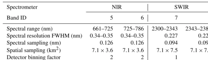
considered a game changer for the determination of atmo-spheric composition from space. TROPOMI is a spaceborne nadir-viewing imaging spectrometer measuring solar radia-tion reflected by the Earth in a push-broom configuraradia-tion. It has a swath width of 2600 km and allows for the analysis of several atmospheric species with an unprecedented level of detail by combining high precision and spatial resolution with daily global coverage. TROPOMI measures radiances between the ultraviolet (UV) and the shortwave infrared (SWIR) in eight bands. The characteristics of the TROPOMI NIR and SWIR bands are summarised in Table 1.
CO and CH4can be retrieved from radiance measurements in TROPOMI’s SWIR bands. For these bands, the spatial res-olution of the nadir measurements is typically 7 km×7 km, which is almost 40 times finer than for SCIAMACHY. In contrast to TANSO, the imaging capabilities of TROPOMI provide 3 orders of magnitude more measurements without gaps, thus facilitating real global maps of CO and CH4in a short time. The unique combination of high precision, spa-tiotemporal resolution, and coverage enables new fields of application. As large sources are readily detected in a single overpass, emission monitoring and air quality assessments are only two examples of the new prospects TROPOMI of-fers. The first applications concerning CO and CH4have al-ready been highlighted and demonstrated in recent publica-tions (Hu et al., 2018; Borsdorff et al., 2018, 2019; Schneis-ing et al., 2019).
As in the fields of weather and climate modelling, ensem-ble approaches have recently acquired an increased impor-tance in the context of satellite observations, aiming at bene-fitting from a larger range of possible realisations of different physical aspects (Reuter et al., 2013) or to analyse to what extent specific geophysical findings depend on the particu-lar characteristics of an algorithm or instrument (Buchwitz et al., 2017). Along these lines, it is worthwhile to have a set of distinct retrieval algorithms for each analysed atmospheric constituent at hand.
Here we introduce a scientific algorithm to retrieve CO and CH4simultaneously from TROPOMI that has the objective of complementing the operational algorithms in the sense described above and to provide new geophysical insights, whilst performing within the mission requirements concern-ing random and systematic errors at the same time. The pre-sented scientific algorithm differs from the operational algo-rithms in several respects (Landgraf et al., 2016; Hu et al., 2016) (see also Sect. 4.1 for a summary of the differences), and the corresponding products are thus predestined to be used together with the operational products in an ensemble approach. After a thorough description of the algorithm, in-cluding error characteristics based on synthetic data and val-idation with independent reference data, we present the first results of our new algorithm for both trace gases,
demon-pave the way.
2 WFM-DOAS retrieval algorithm
The Weighting Function Modified Differential Optical Ab-sorption Spectroscopy (WFM-DOAS) algorithm (Buchwitz et al., 2006, 2007; Schneising et al., 2011, 2014) is a lin-ear least-squares method based on scaling (or shifting) pre-selected atmospheric vertical profiles. The vertical columns of the desired gases are determined from the measured sun-normalised radiance by fitting a linearised radiative transfer model to it. A concise mathematical algorithm description and the key settings and adjustments for the simultaneous CO and CH4retrieval from TROPOMI’s radiance measurements are summarised in the following subsections. The data prod-ucts are based on TROPOMI Level 1b V01.00.00 files com-prising spectra from the nominal operational mode, which started at the end of April 2018, and reprocessed spectra from the previous 6-month commissioning phase. The correspond-ing version is referred to as TROPOMI/WFMD (or WFMD in abbreviated form) v1.2.
2.1 Forward model
The forward model is derived from the radiative transfer model SCIATRAN (Rozanov et al., 2002, 2014) in pseudo-spherical atmosphere mode. To enable a fast retrieval, a lookup table scheme for the radiances and their derivatives has been implemented, containing 17 280 reference spec-tra for varying solar zenith angle, altitude, albedo, water vapour, and temperature. The reference spectra are computed with high spectral resolution in line-by-line mode and subse-quently convolved to the TROPOMI spectral resolution of the SWIR bands using an instrument-specific fixed spectral response function extracted from the TROPOMI ISRF Cali-bration Key Data v1.0.0 for nadir at 2338 nm. The auxiliary input data include US Standard Atmosphere profiles with methane scaled to 1850 ppb, the SCIATRAN aerosol model using the background scenario described in Schneising et al. (2008, 2009), and HITRAN 2016 spectroscopic parameters (Gordon et al., 2017).
2.2 Inversion procedure
scal-Table 1.Summary of the TROPOMI NIR and SWIR spectral bands and their key features (Rozemeijer and Kleipool, 2018).
Spectrometer NIR SWIR
Band ID 5 6 7 8
Spectral range (nm) 661–725 725–786 2300–2343 2343–2389 Spectral resolution FWHM (nm) 0.34–0.35 0.34–0.35 0.227 0.225 Spectral sampling (nm) 0.126 0.126 0.094 0.094 Spatial sampling (km2) 7.1×3.6 7.1×3.6 7.1×7.5 7.1×7.5 Detector binning factor 2 2 1 1
ing factor for the pressure profile, and parameters for a 2nd-order polynomial.
Letm∈Nbe the number of spectral points in the fitting window and n∈Nthe number of state vector elements (fit parameters) with mn. The modelled radiance at wave-lengthλis given by
lnIλmod(v,a)=lnIλmod(v)+ n X
j=1
∂lnIλmod ∂vj vj
(vj−vj)
+Pλ(a), (1)
with state vectorv, linearisation pointv, and polynomial co-efficientsaof 2nd-order polynomialP. A derivative with re-spect to a vertical column thereby refers to the change in the top-of-atmosphere radiance caused by a scaling of a prese-lected absorber concentration vertical profile. There are m
equations of this type, one for each detector pixel in the fit-ting window. The objective is to find the optimal state so that the linear model best fits the observed radiance. This problem can be rewritten as
y=Ax+, (2)
with (log-)radiance difference y∈Rm of the measurement and linearised model due to a deviation x∈Rn of the state vector from the multidimensional linearisation point, weight-ing function (Jacobian) matrix A∈Rm×n (with derivatives at the linearisation point and polynomial basis functions as columns) and the sum of forward model error and (normally distributed log-transformed) instrument noise∈Rm.
The covariance matrix associated with measurement noise is given by Cy=diag(σ12, . . ., σm2)∈Rm×m. To give larger
weight to spectral points with smaller error variances and to obtain error estimates of the retrieval parameters via error propagation from the uncorrelated measurement errorsσi, a
weighted least-squares approach is applied with a matrix of weights defined byW=C−1
y . With the posterior probability p(x|y)of x given y, the most probable inference of the inversionxˆ=arg maxx∈Rnp(x|y)is obtained by minimising
f (x)= W
1
2(y−Ax) 2
2
=(y−Ax)TW(y−Ax) (3) with respect tox, whereT is the matrix transpose. Hence,
∂f (x) ∂x =2
ATWAx−ATWy=! 0 (4)
provides the solutionxˆ =CxATWyof the inverse problem,
whereCx= ATWA
−1
is the covariance matrix of solution ˆ
x. The errors of the retrieval parameters are estimated by
ˆ σj=
q
(Cx)jj. (5)
Due to the potential non-linear dependencies of the radi-ances with respect to water vapour and temperature within their natural variability, the algorithm treats both parameters iteratively. The algorithm starts with lookup table elements representing US Standard Atmosphere water vapour amount and temperature. If the retrieved parameter pair after the fit is closer to another lookup table element, the process is re-peated with the corresponding reference spectrum. Usually convergence is achieved after one iteration step.
As the lookup table only covers direct nadir conditions to limit its dimension to a reasonable size, a geometric path length correction has been implemented to remove the path extension and associated enhancement of the retrieved ver-tical columns for off-nadir conditions with a non-vanishing viewing zenith angle.
Figure 1.Fitting windows (grey, 2311–2315.5 and 2320–2338 nm) and trace gas transmittances for the SWIR bands of TROPOMI for US Standard Atmosphere concentrations. The strong H2O
absorp-tion lines between 2370 and 2380 nm used to obtain cloud informa-tion are shown in light blue . The apparent albedo is retrieved in the continuum at 2313 nm (dashed line).
2.3 Sensitivity and error analysis using synthetic data
The sensitivity of the retrievals to different atmospheric lay-ers is demonstrated by the vertical column averaging ker-nels (Fig. 2). Compared to measurements in the thermal in-frared spectral region, which are primarily sensitive to mid-or upper-tropospheric gas abundances in the absence of high thermal contrast, the advantage of the shortwave infrared spectral region is the sensitivity to all altitude levels, includ-ing the boundary layer, which is important to analyse emis-sions originating from the Earth’s surface.
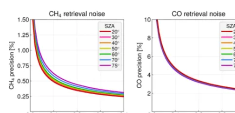
As described in the previous subsection, the retrieval noise is determined via error propagation from the measurement noise. To assess the theoretical precision performance, we assume a simple shot noise-limited noise model, which is defined in the following way: the reference signal-to-noise ratio is SNref=100 in the continuum (radianceLref=4.3× 10¹¹phot s−1cm−2nm−1sr−1) for a dark scene (albedo= 0.05) with low sun (solar zenith angle of 70◦) and is scaled according to
SN(L)=SNref s
L Lref
(6)
for other radiances. The resulting absolute precision is widely independent of the current concentrations. For US Standard Atmosphere values, the corresponding relative re-trieval noise for different albedos and solar zenith angles is shown in Fig. 3. It is below 1 % for solar zenith angles smaller than 75◦ and albedos larger than 0.03 in the case of CH4. As the CO absorption is considerably weaker than the CH4absorption, the CO retrieval exhibits larger relative noise, which is below 8 % for albedos larger than 0.03.
Figure 2.CH4and CO column averaging kernels reflecting the
al-titude sensitivity of the retrievals.
Figure 3.TROPOMI/WFM-DOAS CH4and CO relative retrieval
noise for US Standard Atmosphere conditions.
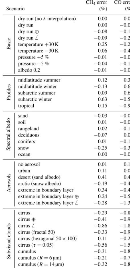
The analysis of systematic errors is performed using sim-ulated measurements. That means that for different scenar-ios defined by specific atmospheric conditions, radiances and irradiances are calculated with the radiative transfer model, which are subsequently used as measurement input in the re-trieval. The errors are then defined as the deviation of the retrieved from the true quantities. The corresponding results for several scenarios are summarised in Table 2. All scenarios already include interpolation between different wavelength grids (for measured and reference spectra) unless otherwise stated.
sce-Figure 4.Spectral albedos of different natural surface types. Re-produced from the ASTER Spectral Library through the courtesy of the Jet Propulsion Laboratory, California Institute of Technology, Pasadena, California (© 1999, California Institute of Technology) and the Digital Spectral Library 06 of the United States Geological Survey.
nario class of profiles includes several realistic model atmo-spheres based on measurements and theoretical predictions (Anderson et al., 1986), with all methane profiles scaled to have surface values of 1850 ppb in each case to better rep-resent current atmospheric conditions. The respective atmo-spheres differ from the US Standard Atmosphere with re-spect to temperature, pressure, water vapour, carbon monox-ide, and methane profiles (see Appendix A of Anderson et al. (1986) for a visualisation of the different vertical profiles). These scenarios are more difficult to deal with than the ba-sic ones because the perturbations are not consistent with the scaling assumption; i.e. they include proper variations of the profile shape.
Also examined is the sensitivity to the spectral albedo of the natural surface types shown in Fig. 4 taken from the Ad-vanced Spaceborne Thermal Emission Reflection Radiome-ter (ASTER) and United States Geological Survey (USGS) spectral libraries. The analysed aerosol scenarios are largely described in Schneising et al. (2008, 2009), with aerosol type definitions in the different atmospheric layers based on Optical Properties of Aerosols and Clouds (OPAC) (Hess et al., 1998). The retrieval errors due to undetected subvi-sual clouds are also investigated for different ice and water clouds.
This gives an impression of the magnitude of errors one can expect, assuming that thick clouds can be filtered out by cloud screening in the preprocessing or post-processing: typ-ical systematic retrieval errors are below 1 % for methane and below 2 % for carbon monoxide, even for challenging scenar-ios.
Figure 5. Systematic retrieval errors for different water clouds (cum.) and ice clouds (cir.) under various conditions.
Larger systematic errors in the case of thick clouds are expected because clouds are not explicitly considered in the forward model of the retrieval algorithm to retain the high processing speed. Therefore, the systematic biases due to clouds are further analysed in more detail. The results for water and ice clouds at different heights are summarised in Fig. 5. Thereby, clouds are modelled as a layer of 1 km ver-tical extent consisting of water droplets with an effective ra-dius of 10 µm or fractal ice crystals with an edge length of 100 µm. The analysis is performed for three different cloud types: two water clouds with cloud-top heights (CTH) of 2 and 4 km and an ice cloud with CTH of 10 km.
As expected, the absolute value of systematic errors typ-ically increases with increasing cloud optical thickness, in-creasing cloud-top height, inin-creasing solar zenith angle, and decreasing albedo. In most cases, there is a considerable underestimation of the vertical column in the case of thick clouds. However, there are also conditions under which the absolute value of the error is small even at a cloud optical thickness ofτ=1 or occasionally turns to an overestimation for measurements over bright surfaces. Overall the system-atic errors due to clouds are qualitatively similar for CO and CH4.
with an effective radiusRof 10 µm.
CH4error CO error
Scenario (%) (%)
Basic
dry run (noλinterpolation) 0.00 0.00 dry run 0.00 −0.03 dry run⊕ −0.08 −0.15 dry run6 −0.09 −0.20
temperature+30 K 0.25 −0.24 temperature−30 K 0.06 −0.42 pressure+5 % −0.01 −0.06 pressure−5 % −0.04 −0.10 albedo 0.2 −0.01 −0.04
Profiles
midlatitude summer 0.12 0.35 midlatitude winter −0.13 0.68 subarctic summer 0.09 0.60 subarctic winter 0.63 −0.59 tropical 0.15 −0.94
Spectral
albedo
sand −0.03 −0.04 soil 0.01 −0.03 rangeland 0.02 −0.11 deciduous −0.07 0.01 conifers 0.01 −0.19 snow −0.25 −0.30 ocean 0.00 −0.07
Aerosols
no aerosol 0.01 0.10
urban 0.11 0.04
desert (sand albedo) 0.41 0.40 arctic (snow albedo) −0.19 −0.41 extreme in boundary layer 0.34 −0.43 extreme in boundary layer⊕ 0.24 −0.51 extreme in boundary layer6 −0.28 −1.38
Sub
visual
clouds
cirrus −0.29 −0.87 cirrus⊕ −0.41 −0.99 cirrus6 −0.86 −1.84 cirrus (fractal 50) −0.33 −0.94 cirrus (hexagonal 50×100) 0.11 −0.20 cirrus (τ=0.05) −0.56 −1.53 cumulus −0.31 −0.86 cumulus (R=6 µm) −0.21 −0.74 cumulus (R=14 µm) −0.32 −0.87 cumulus (τ=0.05) −0.55 −1.44
2.4 High-resolution auxiliary data
As a consequence of the high spatial resolution of the TROPOMI SWIR measurements, a digital elevation model required for the selection and interpolation of suitable pre-calculated reference spectra and a land cover characterisa-tion data set necessary to provide land fraccharacterisa-tion and surface
land fraction, and dominating surface type (Biosphere At-mosphere Transfer Scheme Legend) for every sounding of the satellite.
Some incorrect values of zero elevation in the GMTED2010 data set over the Caspian Sea and Lake Superior have been replaced with corresponding Global 30 Arc-Second Elevation (GTOPO30) values (United States Geological Survey, 2018c). Figure 6 demonstrates the resolution of the implemented elevation and surface type data sets using the example of Europe.
2.5 Post-processing
2.5.1 Column-averaged dry air mole fractions
In order to convert the retrieved vertical columns into column-averaged dry air mole fractions (denoted XCO and XCH4), the columns are divided by the dry air col-umn obtained from the European Centre for Medium-Range Weather Forecasts (ECMWF) analysis. Thereby, the ECMWF dry columns are corrected for the actual surface el-evation of the individual TROPOMI measurements (based on the deviation from the mean altitude of the coarser model grid), inheriting the high spatial resolution of the satellite data.
An analysis based on simulated measurements has indi-cated that this approach is superior to a normalisation by si-multaneously retrieved oxygen (O2A band) from TROPOMI band 6 for off-nadir conditions and/or in the presence of strong scatterers in the atmosphere (aerosol, clouds) as a consequence of the spectral distance in combination with the albedo differences of natural surface types between NIR band 6 and SWIR band 7 (see Fig. 4). For these reasons, O2is a barely sufficient proxy for the light path in the 2.3 µm spec-tral range in a scattering atmosphere. For example, the O2 er-rors for the scattering scenarios aerosols (extreme in bound-ary layer) and clouds (cirrus) from Table 2 are−5.40 % and −7.54 %, respectively. Hence, the O2 underestimations are considerably larger than the corresponding errors for CH4 and CO, which would lead to distinct overestimations of mole fractions obtained from the O2-proxy approach in the presence of strong scatterers.
In addition to the better accuracy of the ECMWF-based mole fraction computation, this approach is also faster be-cause the oxygen fit and the interband coregistration map-ping can be omitted. As a consequence, the fitting procedure is about twice as fast without the normalisation by O2. The out-of-spectral-band stray light issue of the TROPOMI band 6 (Kleipool et al., 2018) would potentially further hamper the O2-proxy approach.
2.5.2 Quality filter
To enable a fast processing speed to handle the huge amount of TROPOMI data, the lookup table is limited to rather simple physical conditions (e.g. cloud-free scenes). Thus, a quality-screening algorithm excluding measurements not sufficiently characterised by the forward model had to be implemented. First of all, challenging conditions with solar zenith angles larger than 75◦, which are increasingly prone to scattering and saturation-related issues due to the weakening signal and lengthening of the light path, are cut off. To be in-dependent of other data sets and their ongoing availability, it was aimed at filtering based on parameters directly included in the retrieval output. This was achieved by using a machine-learning approach based on a random forest classifier, which is a meta estimator growing many independent decision trees on different subsamples of the data set that uses averaging to improve the predictive accuracy and prevent overfitting. Thereby, each tree of the ensemble is grown in the following way (Breiman, 2001).
1. Randomly drawNsamples from the training set of size
N with replacement (bootstrap sample). For largeN, a fraction of about 63.2 % unique samples is expected, the remainder being duplicates.
2. From the F input variables, f F features are ran-domly chosen out ofF, and the best split according to the minimisation of Gini impurity on theseffeatures is used to split the node (Breiman, 1996a). The value off
is held constant during the forest growing.
3. There is no pruning of the decision trees; i.e. each tree is grown to the largest possible extent.
To classify a new previously unseen measurement after growing the forest with the training data, each decision tree gives a classification according to the input features of the measurement, and the forest chooses the majority vote over all trees in the forest. The combination of the tree results, each based on different bootstrap replicates of the learn-ing set, is called bootstrap aggregatlearn-ing or bagglearn-ing (Breiman, 1996b). The forest error rate depends on the correlation be-tween the trees in the forest and the strength of the individual trees. The forest error rate decreases with decreasing corre-lation and increasing strength of the trees. Reducingf re-duces both the correlation and the strength, while increasing
f increases both. Hence, there is an optimal range off that minimises the forest error rate.
We use a forest size of 200 trees and the well-recognised standard choice off =
√
Figure 6.USGS GMTED2010 elevation and GLCC surface type (Biosphere Atmosphere Transfer Scheme Legend) with 0.05◦resolution using the example of Europe. The Biosphere Atmosphere Transfer Scheme Legend comprises the following surface types (United States Ge-ological Survey, 2018a): 1 crops, mixed farming; 2 short grass; 3 evergreen needleleaf trees; 4 deciduous needleleaf trees; 5 deciduous broadleaf trees; 6 evergreen broadleaf trees; 7 tall grass; 8 desert; 9 tundra; 10 irrigated crops; 11 semidesert; 12 ice caps and glaciers; 13 bogs and marshes; 14 inland water; 15 ocean; 16 evergreen shrubs; 17 deciduous shrubs; 18 mixed forest; 19 forest–field mosaic; 20 wa-ter and land mixtures. In the GMTED2010 data set, ocean areas have been assigned a value of 0 (shown in dark blue).
training subset consists of 80 million measurements, which are classified based on cloud information from the Visible Infrared Imaging Radiometer Suite (VIIRS) onboard Suomi NPP (Hutchison and Cracknell, 2005), which flies in loose formation configuration with Sentinel-5 Precursor (S5P trails behind by 3.5 min). This classification is augmented by addi-tionally flagging distinct XCH4 deviations relative to a cli-matology consisting of averages on a 6◦×4◦ grid for the years 2003–2005 based on the MACC-II flux inversion sys-tem (Bergamaschi et al., 2013) and adjusted by an accumu-lated increase until the time of the measurement based on globally averaged marine NOAA surface data (Dlugokencky, 2018), identifying scenes obviously not well-characterised by the forward model, in particular conspicuously decreased methane abundances in the presence of clouds due to shield-ing of the underlyshield-ing atmosphere or in the case of very low surface reflectances.
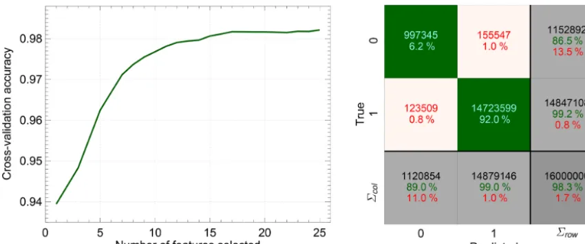
To train the forest, a set F of 25 feature variables is se-lected by feature ranking with recursive feature elimination and cross-validated selection of the best features. As widely used, 20 % of the training data is randomly drawn and re-tained as test data (e.g. Suthaharan, 2016; Hino et al., 2018). The corresponding predictive accuracy is shown in Fig. 7 as a function of the selected features, confirming that the random forest does not overfit because the accuracy has its global maximum when using all 25 features as listed below. The se-lected variables in order of importance are (1) H2O column difference to the ECMWF, (2) cloud parameterrcld, (3) sim-plified surface type (water, coastal, land, desert, ice), (4) lin-ear polynomial coefficientp1, (5) pressure difference to the
ECMWF, (6) altitude, (7) latitude, (8) CO fit error, (9) tem-perature, (10) root mean square of fit residual, (11) tempera-ture difference to the ECMWF, (12) H2O fit error, (13) pres-sure fit error, (14) H2O column, (15) longitude, (16) solar zenith angle, (17) pressure, (18) quadratic polynomial coef-ficient p2, (19) radiance ratio of strong H2O absorption to continuum, (20) dry air column from the ECMWF, (21) re-trieved apparent albedo, (22) continuum radiance, (23) rel-ative azimuth angle, (24) across-track dimension index, and (25) strong H2O absorption radiance. The predictive accu-racy when using all 25 features amounts to 0.983, which means that 98.3 % of all scenes are correctly classified.
Figure 7. Cross-validated predictive accuracy of the quality classification random forest obtained by recursive feature elimination. The confusion matrix when using all 25 features is shown on the right-hand side for the test data set, denoting good observations with 0 and measurements to be excluded with 1. The green diagonal cells correspond to correct classifications and the red off-diagonal cells to incorrect classifications. The number of scenes and the percentage of the total number of scenes are given in each cell. Important key parameters are summarised in the grey cells along the edge. The right column shows the percentages of all the elements belonging to each class that are correctly (recall) and incorrectly (false negative rate) classified and the bottom row those that are predicted to belong to each class that are correctly (precision) and incorrectly (false discovery rate) classified. The dark grey cell in the bottom right corner displays the overall accuracy.
these cases the filter appears not stringent enough. However, as the training classification is quite strict, that does not nec-essarily mean that all these measurements are actually of low quality. The rate can rather be interpreted as an upper bound of potentially remaining challenging retrievals on the verge of sufficient characterisation by the forward model, e.g. ob-servations near cloud edges. The effective diagnostic perfor-mance of the quality filter will emerge from the validation.
Adding additional parameters toF does not significantly improve the predictive accuracy further. It is important to note that the resulting classification is independent of the ab-solute abundances of the primary retrieval parameters CH4 and CO. The performance of the classification algorithm is demonstrated in Fig. 8, confirming that cloudy scenes are re-liably excluded in general and that the quality filter is usually stricter than the VIIRS classification, in particular over the weakly reflecting ocean. Measurements classified as cloudy by VIIRS but still passing the quality filter are rare and not associated with conspicuous methane abundances.
2.5.3 Shallow learning calibration for methane
The implemented machine-learning-based quality filter de-scribed in the previous subsection removes observations not sufficiently characterised by the forward model. Although this procedure typically excludes scenes exhibiting large sys-tematic errors, smaller syssys-tematic errors may remain in the residual data set. In particular, there seems to be a systematic albedo dependence of unknown origin of retrieved methane abundances with an underestimation over dark surfaces. As
a consequence of the fairly stringent quality requirements for methane, a random forest regressor algorithm was imple-mented to reduce the remaining systematic methane errors after the retrieval by calibrating against an assumed stan-dard defined below, which is deemed insensitive to surface reflectance variations.
Like the classification algorithm described in the previous subsection, the random forest regressor (Criminisi and Shot-ton, 2013) grows an ensemble of decision trees, training each tree on a different data sample by applying the bootstrap ag-gregating technique. From thef randomly chosen parame-ters the optimal split maximising the variance reduction in the child nodes is used to split the nodes. To focus on the most prominent features (shallow learning of systematic er-rors caused by surface albedo variations), the tree growing is limited to 500 leaf nodes. Again, a forest size of 200 trees and
f = √
Figure 8. (a, b)Quality-filtered XCH4over Europe overlaid on true colour reflectances from the Visible Infrared Imaging Radiometer Suite
(VIIRS) taken from the NASA Worldview application for two example days not included in the training data set, demonstrating the perfor-mance of the machine-learning classification algorithm. Evidently, cloudy scenes are typically identified and excluded.(c, d)Comparison of the implemented quality filter (QUAL, 1: excluded) with the VIIRS cloud classification (1: cloudy). Matching classifications are shown in white and green. By definition the quality filter is generally stricter than the VIIRS cloud flag and the blue areas are additionally excluded. The rare instances of measurements classified as cloudy by VIIRS but still passing the quality filter are shown in cyan.
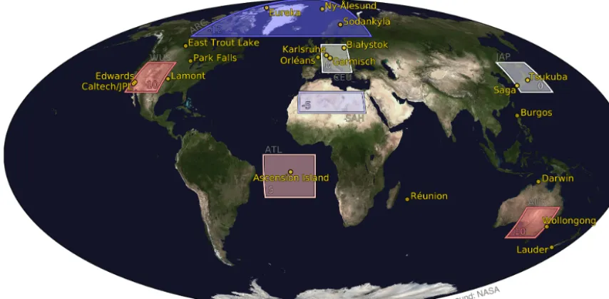
The calibration data set consists of the XCH4climatology introduced in the previous subsection evaluated for selected regions spanning a wide range of albedos and solar zenith an-gles. For individual regions, the climatology is roughly cor-rected for potential systematic overall biases by adding up a single region-specific correction value based on a compari-son to nearby sites of the Total Carbon Column Observing Network (TCCON) (Wunch et al., 2011a) for the year 2017. In any case, the seasonal and intra-regional spatial variations are solely determined by the climatology. The training re-gions and corresponding climatology correction values are shown in Fig. 9.
The standard deviation of the resulting XCH4correction when considering global yearly averages of gridded data (on
a 0.1◦×0.1◦grid) amounts to 13 ppb, which is well below the natural variability. The XCO data set is not corrected.
3 Validation
scal-Figure 9.Regions used to train the machine-learning regressor comprising the Arctic (ARC), the western United States (WUS), central Europe (CEU), Japan (JAP), the Sahara (SAH), the South Atlantic (ATL), and Australia (AUS). The corresponding numbers specify the regional corrections applied to the methane climatology before learning in parts per billion, which are also colour-coded in the borders and backgrounds of the regions (blue for negative and red for positive corrections). The yellow circles highlight the TCCON sites used in the validation.
ing factors for each species. The estimated accuracy (1σ) is about 2 ppb for XCO and 3.5 ppb for XCH4 (Wunch et al., 2010).
To compare the satellite data with TCCON quantitatively, it has to be taken into account that the sensitivities of the in-struments differ from each other and that individual a priori profiles are used to determine the best estimate of the true atmospheric state, respectively. The first step is to correct for the a priori contribution to the smoothing equation by adjusting the measurements for a common a priori profile (Rodgers, 2000; Schneising et al., 2012; Dils et al., 2014). Here we use the TCCON prior as the common a priori pro-file for all measurements:
ˆ
cadj= ˆc+ 1
m0 X
l
ml(1−Al)
xal,T−xal (7)
In this equation, cˆ represents the originally retrieved TROPOMI column-averaged dry air mole fraction, l is the index of the vertical layer,Al the corresponding column
av-eraging kernel of the TROPOMI algorithm, andxaandxa,T the TROPOMI and TCCON a priori dry air mole fraction profiles; ml is the mass of dry air determined from the dry
air pressure difference between the upper and lower bound-ary of layerlvia 1pl
gl with gravitational accelerationgl and
m0=Plml is the total mass of dry air. To minimise the
smoothing error introduced by the averaging kernels we do not compare cˆadj directly with the retrieved TCCON mole fractionscˆTbut rather with the adjusted expression (Rodgers
and Connor, 2003; Wunch et al., 2011b):
ˆ
cT,adj=ca,T+ cˆ
T
ca,T −1
1
m0 X
l
mlAlxal,T. (8)
Thereby, ca,T represents the TCCON a priori column-averaged dry air mole fraction associated with the a priori profile xa,T. However, using cˆT,adj instead of cˆT has only a marginal impact on the validation results presented here because the satellite averaging kernels are close to 1 in the lower atmosphere (see Fig. 2), implyingcˆT,adj≈ ˆcT.
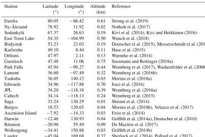
The validation is performed at the TCCON sites listed in Table 3 (see also Fig. 9). For the comparison a set of colloca-tion criteria has to be specified. Ideally, the representativity is maximised by criteria that are as strict as possible while concurrently ensuring sufficient data for a sound and stable comparison. This trade-off is resolved by the following se-lection. The spatial collocation criterion requires the satellite measurements to lie within a radius of 100 km around the TCCON site and the altitude difference to be smaller than 250 m. The temporal collocation criterion is set to±2 h. As a consequence of the altitude representativity criterion, there are not enough collocations for a robust comparison at the mountain sites Zugspitze (Sussmann and Rettinger, 2018b) and Izaña (Blumenstock et al., 2017).
( ) ( ) (km)
Eureka 80.05 −86.42 0.61 Strong et al. (2019) Ny-Ålesund 78.92 11.92 0.02 Notholt et al. (2017)
Sodankylä 67.37 26.63 0.19 Kivi et al. (2014); Kivi and Heikkinen (2016) East Trout Lake 54.35 −104.99 0.50 Wunch et al. (2018)
Białystok 53.23 23.03 0.19 Deutscher et al. (2015), Messerschmidt et al. (2012) Karlsruhe 49.10 8.44 0.11 Hase et al. (2015)
Orléans 47.97 2.11 0.13 Warneke et al. (2014)
Garmisch 47.48 11.06 0.75 Sussmann and Rettinger (2018a)
Park Falls 45.94 −90.27 0.44 Wennberg et al. (2017), Washenfelder et al. (2006) Lamont 36.60 −97.49 0.32 Wennberg et al. (2016b)
Tsukuba 36.05 140.12 0.03 Morino et al. (2018a) Edwards 34.96 −117.88 0.70 Iraci et al. (2016) JPL 34.20 −118.18 0.39 Wennberg et al. (2016a) Caltech 34.14 −118.13 0.24 Wennberg et al. (2015) Saga 33.24 130.29 0.01 Shiomi et al. (2014)
Burgos 18.53 120.65 0.04 Morino et al. (2018b), Velazco et al. (2017) Ascension Island −7.92 −14.33 0.03 Feist et al. (2014)
Darwin −12.46 130.93 0.04 Griffith et al. (2014a), Deutscher et al. (2010) Réunion −20.90 55.49 0.09 De Mazière et al. (2017)
Wollongong −34.41 150.88 0.03 Griffith et al. (2014b)
Lauder −45.04 169.68 0.37 Sherlock et al. (2014), Pollard et al. (2017)
against outliers of a normal distribution. This is an appropri-ate choice and preferred over the standard deviation because one is interested in the actual single-measurement precision without distortion of the results by a few outliers, which are rather attributed to systematic errors, e.g. due to resid-ual clouds. As a consequence, outliers are fully included in the computation of the systematic error but get lower weight in the robust determination of the random error, which is in-terpreted as a measure of the repeatability of measurements. It is also checked whether the respective site biases are sensitive to the selection of the spatial collocation radius, which is an indication of sources within the satellite colloca-tion area with only a marginal influence on the TCCON mea-surements themselves. A considerable sensitivity was found for XCH4 at Edwards. The collocation region intersects oil production areas in California’s Central Valley (in contrast to Caltech and JPL; see also the results in Sect. 4 and Fig. 23) and the South Coast Air Basin (SoCAB), which has a well-known methane enhancement (Wunch et al., 2016). As such nearby sources limit the representativity of affected satellite measurements, the collocation radius is reduced to 50 km for Edwards.
The altitude representativity criterion separates the well-isolated air masses of the SoCAB, where Caltech and JPL are located, from the Mojave desert with the Edwards site to the north. Hence, different air masses are analysed in the valida-tion at Caltech/JPL and Edwards, although the corresponding collocation circles overlap. This also explains the insensitiv-ity to the spatial collocation radius at Caltech/JPL and why
no additional constraints on the coincidence criteria are nec-essary for these sites to ensure representativity. As Caltech and JPL are both exposed to SoCAB air masses, the permis-sible altitude collocation tolerance of Caltech is equally as-sumed for JPL despite slightly differing surface elevation.
The results for the individual sites are condensed to the following parameters for the overall quality assessment of the satellite data: the global offset is defined as the mean of the local offsets at the individual sites, the random error is the global scatter (analogously estimated to the single-site case) of the differences to TCCON after subtraction of the respective regional biases, and the systematic error is the standard deviation of the local offsets relative to TCCON at the individual sites as a measure of the station-to-station biases. For XCO the global offset amounts to 4.49 ppb, the random error is estimated to be 5.14 ppb (6.12 ppb when us-ing the standard deviation instead of Huber’s Proposal-2 M-estimator), and the systematic error is 1.90 ppb, which is on the order of the estimated (station-to-station) accuracy of the TCCON of about 2 ppb. For XCH4the global offset aggre-gates to−1.30 ppb, the random error is 14.04 ppb (15.77 ppb when using the standard deviation), and the systematic error is given by 4.31 ppb, which is again similar to the TCCON accuracy of about 3.5 ppb.
Figure 10.Comparison of the TROPOMI/WFMD v1.2 XCO time series (green) with ground-based measurements from the TCCON (red). For each site,Nis the number of collocations,µcorresponds to the mean bias, andσ to the scatter of the satellite data relative to TCCON in parts per billion;σ is estimated from Huber’s Proposal-2 M-estimator. The global offset is defined as the mean of the local offsets at the individual sites, the random error is the global scatter of the differences to TCCON after subtraction of the respective regional biases, and the systematic error is the standard deviation of theµat the individual sites.
andR=0.91 for XCH4) underlines the typically good agree-ment of the satellite and validation data. The linear regression yields a fit close to the 1:1 line for both gases.
In the case of XCH4, there are a few outliers for which the satellite values are considerably lower than the TCCON val-ues. These occasional instances are not site-specific and can probably be ascribed to days with residual or partial cloud cover interfering with the satellite retrievals. Outliers with
Figure 11.As Fig. 10 but for XCH4.
stratospheric part of the methane profile may be largely af-fected by the polar vortex, leading to a considerable deviation from the assumed a priori profile shapes (Tukiainen et al., 2016). It is verified that the impact of outliers on the regres-sion is marginal by repeating the fit with the Huber linear regression model (Huber and Ronchetti, 2009), which is ro-bust to outliers and provides similar results to the standard linear regression here.
In summary, the natural XCH4 and XCO variations are well-captured by the satellite data. We find a single-measurement precision of the TROPOMI data of about 0.8 %
for XCH4and 5.8 % for XCO, while the station-to-station ac-curacy of the satellite data is comparable to the TCCON.
4 Initial results using real TROPOMI data
Figure 12.Comparison of the TROPOMI/WFMD data to the TCCON based on daily means. Specified are the linear regression results and the correlation of the data sets, as well as the mean and standard deviation of the difference. To analyse the impact of outliers, the regression is also performed for the Huber linear regression model, which is robust to outliers.
The global distribution of retrieved XCO and XCH4for the year 2018 is shown in Figs. 13 and 14, respectively. Clearly visible is the interhemispheric gradient with larger values on the Northern Hemisphere, where the majority of sources is located, for both data sets superimposed by enhancements over prominent source regions like anthro-pogenic emissions in China, India, and Southeast Asia.
Other visible XCO source regions include human-initiated biomass burning in Africa and South America for land clear-ing and land use change, as well as wildfire emissions in North America, which were exceptionally pronounced in 2018. The anthropogenic emissions of congested urban ar-eas like Mexico City and Tehran are already unambiguously detected on such a global map without zooming in.
In the case of XCH4additional visible source regions apart from the anthropogenic sources in Asia, like fossil fuels or rice cultivation, include tropical wetlands and anthropogenic emissions from California and the Padan Plain in Italy. There is also a distinct signal from Etosha National Park in the north of Namibia containing significant areas of wetland like the Etosha pan, an endorheic salt pan that exhibits intermittent shallow inundation.
4.1 Comparison to operational products
The operational TROPOMI CO product is retrieved using the Shortwave Infrared CO Retrieval (SICOR) algorithm (Landgraf et al., 2016), and the operational CH4product is based on RemoTeC (Hu et al., 2016), which is a physics-based approach originally developed for CO2 and CH4 re-trievals from OCO and GOSAT. Although the operational al-gorithms and the scientific algorithm presented here use simi-lar spectral bands, there are many differences concerning the details of each approach. For example, TROPOMI/WFMD
is a weighted least-squares approach, whereas SICOR and RemoTec are based on a Philips–Tikhonov regularisation scheme. There are also differences in the radiative transfer model, the quality filter, the spectroscopy used, and the state vector elements, in particular in the treatment of aerosols and clouds.
While WFMD and the operational CH4 algorithm are mainly applicable to cloud-free scenes, the operational CO algorithm is designed to also handle cloudy observations un-der specific conditions. Both methane algorithms include a post-processing correction to improve the systematic albedo dependence. However, the details of this correction are again quite different: while the correction for the operational al-gorithm is based on linear regression relative to GOSAT re-trievals, which are in turn bias-corrected against TCCON, the scientific WFMD algorithm uses a random forest regressor relative to a climatology as described in Sect. 2.5.3.
Figure 13.Global yearly average of TROPOMI/WFMD XCO for 2018.
Figure 14.Global yearly average of TROPOMI/WFMD XCH4for 2018.
WFMD, which is also reflected in a regression slope some-what smaller than 1.
The corresponding comparison of the CH4 results is shown in Figs. 16 and 17 for December and June 2018, re-spectively. WFMD exhibits somewhat better coverage and also includes some retrievals over the ocean in contrast to the operational algorithm. Although the prominent features, like
stan-Figure 15.Comparison of TROPOMI/WFMD CO with the operational TROPOMI data for December 2018. Panel(a)depicts the global distribution of all quality-filtered data for the respective algorithm. Panel(b)shows a bivariate histogram of all common scenes passing the quality filters of both algorithms, summarising the linear regression results and the correlation of the data sets, as well as the mean and standard deviation of the difference. The number of points per bin is shown as a decadic logarithm lg(N ).
dard deviation of the difference is again comparable to the noise level.
In December 2018 the methane abundances over the Bo-hai Economic Rim, including the cities of Beijing and Tian-jin, are larger than in southern China to the west of the Pearl River Delta for WFMD, whereas it is the other way round for the operational product, but this may be due to the different sampling. The XCH4 distribution over the Sahara is more uniform for WFMD, and the corresponding patterns of the operational product seem to vaguely resemble some albedo features, with higher values over brighter parts of the Sahara. There is an obvious clustering of the common measurements around the 1:1 line, even for the largest values. Neverthe-less, the linear regression line is somewhat distorted from the 1:1 line due to a slight shift of the two dominating densely populated sub-clusters.
In June 2018 there is a sharper XCH4 gradient in the operational product when transitioning from the temperate into the low albedo boreal zone, and the values over the bo-real ecosystem are lower than for WFMD. In addition, there are enhanced methane abundances in the operational product over the Canadian province Nunavut in contrast to WFMD. Some occasionally high values in the WFMD methane data over South America possibly attributable to surface rough-ness contribute to the rare outliers in the comparison scatter plot, which exhibits a clear linear relation close to the 1:1 line apart from that.
Overall, we find good agreement of our scientific CO prod-uct with the operational prodprod-uct based on the presented con-cise comparison. For CH4 we find good agreement of the
prominent features with some interesting differences in de-tail, including potential indications of residual albedo issues in the operational XCH4 product. Further future analysis and understanding of the differences is expected to advance greenhouse gas retrievals from wide-swath imaging satellites like TROPOMI under challenging conditions such as scenes with low surface reflectance or residual cloudiness.
4.2 Detection of emission sources 4.2.1 Carbon monoxide
Intense CO emissions from agglomeration areas, cities, and industrial facilities are clearly detected by TROPOMI. This is demonstrated using the example of China, India, and South-east Asia in Fig. 18. The 2-month average was chosen to get an overview of the complete region. Typically, larger emis-sions can even be detected in a single satellite overpass. The tracked facilities mainly belong to the Chinese and Indian iron and steel industry.
prod-Figure 16.As Fig. 15 but for methane.
Figure 17.As Fig. 16 but for June 2018.
uct. A possible reason for this is the additional utilisation of cloudy observations in the operational SICOR product, which may be associated with reduced surface sensitivity un-der certain conditions reflected in the averaging kernels of the corresponding measurements.
In steelmaking CO is formed during two processes. Firstly, it is an essential constituent of blast furnace gas, which emerges when iron ore is reduced with coke to metallic pig iron. As the resulting pig iron has a relatively high carbon content, further processing is necessary to harden the metal. Therefore, the carbon-rich molten pig iron is converted to steel by lowering its carbon content via oxidation in the
oxy-gen converter process (Linz–Donawitz steelmaking). The re-sulting converter gas predominantly consists of CO (≈70 %) (Ishioka et al., 1992; CarbonNext, 2017).
Figure 18.Carbon monoxide distribution for November and December 2018 over China, India, and Southeast Asia highlighting emissions from congested urban areas and industrial facilities. Panel(a)shows the TROPOMI/WFMD product and panel(b)the operational product.
Company (NALCO), the Tang Loong Industrial Park in Viet-nam, and the cement production plants of the Arco Group and Khyber Industries in the Kashmir Valley, where CO ac-cumulates between the mountain ranges.
CO emissions from the steel industry can also be observed in other regions of the world, for example in Turkey. Fig-ure 19 shows that two of the largest steel plants in the country are detected in a single satellite overpass. The plants are
Figure 19.Carbon monoxide enhancement due to emissions from steel plants in Turkey.
There are also examples of detected CO emissions from steel works in Europe. Figure 20 illustrates such a case and shows that CO emissions from the largest steel plant in Poland, operated by ArcelorMittal in the industrial city D ˛abrowa Górnicza in the Upper Silesian metropolitan area, are detected in a single overpass. As can be seen, the cor-responding pronounced plume coincides with the boundary layer wind direction, and the striping is observable as well.
Another prominent source of CO is fire. In Septem-ber 2018 a peat bog in the military training area WTD 91 in the Emsland region was accidentally set on fire by the Ger-man army and burnt for several weeks. The corresponding CO plume is clearly detected and aligns well with the wind direction (Fig. 21). The scenes right above the origin of the fire are automatically excluded by the quality filter because of the strong formation of smoke potentially shielding the subjacent partial columns, similar to thick clouds.
The difference between smoke and clouds is the parti-cle size distribution. While clouds consist of water droplets with an effective radius of about 10 µm, the mass distribution of smoke plumes shows a prominent peak at about 0.3 µm (Stith et al., 1981) but is nevertheless dominated by a small number of supermicron-sized particles (Radke et al., 1990). The submicron particles reduce visibility and lead to an ex-tended smoke plume over large distances in the true colour reflectances from VIIRS shown in Fig. 21. However, these small particles are not a major issue for the satellite measure-ments taken at 2.3 µm. The satellite retrievals near the origin of the fire are rather affected by the large supermicron-sized particles, which become more and more negligible when
de-parting from the source of the fire due to their rapid fallout. This is the reason that at a sufficient distance from the fire the corresponding measurements pass the quality filter de-spite efficient scattering in the visible spectral range mani-festing in an extensive plume in the VIIRS image. On the other hand, even very small clouds, which are barely visible in the VIIRS image at this resolution, are rigorously filtered out. This indicates that the algorithm implicitly distinguishes between smoke and clouds according to their particle sizes and that a reliable CO retrieval is possible in smoke plumes in the far field of the fire origin. A thorough discussion of the sensitivity of CO measurements in conjunction with smoke from fires can be found in the revised version of Schneising et al. (2019).
The total column enhancementE relative to background values allows us to roughly estimate the emitted mass flux
8of CO from the mean boundary layer wind speedv and the plume widthx⊥perpendicular to the wind direction only using measurements passing the quality filter:
8=E·v·x⊥. (9)
The plume width is on the same order of magnitude as the instrument’s spatial resolution, and the enhancement is thus calculated for the plume scene passing the quality filter which is nearest to the fire origin. As the wind direction is approximately perpendicular to one of the scene diagonals, the corresponding plume widthx⊥ is estimated by √a
2, as-suming a quadratic scene with a side lengthaof about 7 km. WithE=(7±0.7)×1017molec cm−2,v=12±3 m s−1, and
Figure 20.Carbon monoxide enhancement due to emissions from the ArcelorMittal steel plant in D ˛abrowa Górnicza in the Upper Silesian metropolitan area in Poland. Also shown is the mean wind in the boundary layer obtained from ECMWF data.
about 8=1.7±0.6 ktCO. According to Kohlenberg et al. (2018), a CO : CO2 emission factor of 16±3 % for boreal peat fires is assumed, implying an associated CO2emission of approximately 10.5±4.0 ktCO2on that day. Compared to the German yearly total budget of about 800 MtCO2yr−1, the emissions from the Emsland peat fire are small even if one assumes that the fire burnt for several weeks at this strength.
4.2.2 Methane
One integral component of anthropogenic methane sources is emissions from the energy sector. As an example of methane leakage from natural gas production, Fig. 22 shows that the emissions of the world’s second-largest natural gas field, Galkynysh in Turkmenistan, which is operated by Türk-mengaz, can be clearly detected in a single satellite overpass. Also visible are XCH4 enhancements over the productive South Caspian oil and gas basins, the oil and gas infrastruc-ture at the Turkmen coast of the Caspian Sea, and smaller oil and gas fields south of Galkynysh.
Emissions from oil and gas production are important to monitor because methane leaks offset the climate change benefits of natural gas or oil over coal if the leakage ex-ceeds a certain threshold (Alvarez et al., 2012; Farquharson et al., 2016). There are several studies suggesting that the oil and gas industry leaks more methane than assumed in in-ventories, at least locally or temporally (Brandt et al., 2014; Schneising et al., 2014; Alvarez et al., 2018), and the
poten-tial heterogeneity among the sector complicates the specifi-cation of typical emission rates.
Another source region is the Central Valley in California, with combined anthropogenic emissions from oil fields and agriculture (see Fig. 23). While one main area of oil pro-duction is located in Kern County around Bakersfield, the dairy and cattle industry extends more or less over the whole valley, with the largest livestock density in the counties of San Joaquin, Stanislaus, Merced, Kings, and Tulare (Mauger et al., 2015). A reliable disentanglement of the emissions from the oil and agriculture sectors requires exact knowl-edge of the meteorology and unmistaken prior knowlknowl-edge of the distribution of the different source types or methane isotopologue information, which is not yet available from satellite observations. As already mentioned in Sect. 3, the 100 km collocation radius standardly used in the validation intersects the Kern County source region for the Edwards TCCON site. As a consequence, the collocation radius is re-duced to 50 km for Edwards to ensure the representativity of the satellite measurements used in the validation.
The two hitherto presented methane source regions of Turkmenistan and the Central Valley in California, which are both detected in a single TROPOMI overpass, were already identified in yearly averages of SCIAMACHY data (Buch-witz et al., 2017).
Figure 22.Methane enhancement due to emissions from the world’s second-largest natural gas field, Galkynysh in Turkmenistan.
Required Achieved Required Achieved Carbon monoxide (CO) Total column 15 2.1 10 5.8 Methane (CH4) Total column 1.5 0.2 1.0 0.8
Figure 24.Methane distribution over the Upper Silesian Coal Basin in Poland. Individual mines are highlighted by red hexagons.
adsorbed at coal grains. For safety reasons, the coal mine methane is diluted with air below the explosive range and released through ventilation shafts to the surface.
Poland’s primary energy consumption and electrical power generation relies strongly on coal, which helped the country to achieve one of the lowest energy import depen-dencies in the European Union (European Statistical Office, 2018) as measured by the share of net imports in gross inland energy consumption (the sum of energy produced and net im-ports). The energy dependence rate of Poland was about 30 % in 2016 compared to an EU-wide average of 54 %, meaning that the majority of the EU’s energy needs are met by net imports. Only three EU countries have a lower energy de-pendence rate than Poland, namely Romania, Denmark, and Estonia.
Poland is the largest coal-mining country in Europe and among the top 10 coal producers in the world (BP, 2018), with huge reserves of hard coal and lignite (Polish Geolog-ical Institute, 2018a, b). The major coal basin is the Upper Silesian Coal Basin (USCB), which is larger than 5000 km2 and hosts 80 % of the anticipated domestic hard coal re-sources. All operating hard coal mines in the country are
sit-uated in the USCB except the Bogdanka Mine in the Lublin Coal Basin in the east of Poland. The USCB is shown in Fig. 24, highlighting individual mines. The corresponding methane plume is vaguely perceptible and coincides with the wind direction. This is an example of emissions that are ob-viously close to the detection limit for a single overpass.
5 Conclusions
are no longer needed in the actual quality prediction of indi-vidual previously unseen measurements after the completion of the training, the quality filter is independent of the con-tinuous availability of external cloud information. The per-formance of the retrieval algorithm is expected to further im-prove in the future, for example with respect to striping in flight direction for single overpasses, due to a refined calibra-tion of the TROPOMI instrument and/or dedicated algorithm advancements.
The good global agreement of our scientific products with the operational products for the analysed example cases fur-ther underlines the quality of the presented algorithm. The differences in detail for XCH4can be thought of as a stimu-lation for further future analysis. The understanding of these differences will likely allow us to symbiotically advance both retrieval algorithms under challenging conditions, such as scenes with low surface reflectance or residual cloudiness. Moreover, the scientific and operational products are predes-tined to be used together with other products in an ensemble approach to benefit from the large range of respective realisa-tions of different physical aspects in the individual retrieval algorithms.
Nevertheless, the results of the presented scientific algo-rithm are also valuable in their own right, as TROPOMI en-ables the determination of XCO and XCH4with an unprece-dented level of detail on a global scale, introducing new areas of application. It was shown that CO emissions from agglom-eration areas, industrial facilities, in particular from the steel industry, and fires are readily detected, often even in a sin-gle satellite overpass. The same is true for CH4 emissions from the energy sector, including leakage from oil and gas production and coal bed methane from coal mining. The fu-ture quantitative reinforcement of these primarily qualitative findings will potentially enable emission monitoring and air quality assessments, ideally on a daily recurrent basis. Fur-thermore, improved knowledge of the methane cycle, which is essential for better prediction of future climate, can be de-rived by combining inverse modelling with a comprehensive monitoring system comprising complementary information from accurate ground-based in situ measurements and satel-lite observations with a unique combination of high preci-sion, spatiotemporal resolution, and global coverage.
Data availability. The carbon monoxide and methane data sets presented in this publication can be accessed via http://www. iup.uni-bremen.de/carbon_ghg/products/tropomi_wfmd/ (Schneis-ing, 2019, last access: 25 November 2019).
Author contributions. OS designed and operated the TROPOMI/WFMD satellite retrievals, performed the data analysis, interpreted the results, and wrote the paper. MB, MR, HB, and JPB provided significant conceptual input to the design of the TROPOMI/WFMD satellite retrievals, the interpretation, and
the improvement of the paper. TB and JL designed and executed the operational TROPOMI CO and CH4 satellite retrievals and
supported the interpretation of the results. NMD, DGF, DWTG, FH, CH, LTI, RK, IM, JN, CP, DFP, SR, KeS, KiS, RS, VAV, TW, and DW operated the TCCON retrievals for the various sites and supported the interpretation of the results. All authors discussed the results and commented on the paper.
Competing interests. The authors declare that they have no conflict of interest.
Special issue statement. This article is part of the special is-sue “TROPOMI on Sentinel-5 Precursor: first year in operation (AMT/ACP inter-journal SI)”. It is not associated with a confer-ence.
Acknowledgements. This publication contains modified Coperni-cus Sentinel data (2017, 2018). Sentinel-5 Precursor is an ESA mission implemented on behalf of the European Commission. The TROPOMI payload is a joint development by the ESA and the Netherlands Space Office (NSO). The Sentinel-5 Precursor ground-segment development has been funded by the ESA and with na-tional contributions from the Netherlands, Germany, and Belgium. The research leading to the presented results has in part been funded by the ESA projects GHG-CCI, GHG-CCI+, and S5L2PP, the Fed-eral Ministry of Education and Research project AIRSPACE, and by the State and the University of Bremen.
B, C, D). The Lauder TCCON programme is core-funded by the NIWA through New Zealand’s Ministry of Business, Innovation and Employment. JN, CP, and TW acknowledge financial support by the DFG within Transregio (AC)3.
We acknowledge the use of VIIRS imagery from the NASA Worldview application (https://worldview.earthdata.nasa.gov/, last access: 9 September 2019) operated by the NASA/Goddard Space Flight Center Earth Science Data and Information System (ESDIS). We also thank the European Centre for Medium-Range Weather Forecasts (ECMWF) for providing the meteorological analysis and Peter Bergamaschi for providing the MACC-II project flux inver-sion system methane mole fractions used to generate the utilised XCH4climatology.
Financial support. The research leading to the presented re-sults has in part been funded by the ESA projects GHG-CCI, GHG-CCI+, and S5L2PP, the Federal Ministry of Education and Research project AIRSPACE, and by the State and the University of Bremen.
The article processing charges for this open-access publica-tion were covered by the University of Bremen.
Review statement. This paper was edited by Helen Worden and re-viewed by two anonymous referees.
References
Alvarez, R. A., Pacala, S. W., Winebrake, J. J., Chameides, W. L., and Hamburg, S. P.: Greater focus needed on methane leakage from natural gas infrastructure, P. Natl. Acad. Sci. USA, 109, 6435–6440, https://doi.org/10.1073/pnas.1202407109, 2012. Alvarez, R. A., Zavala-Araiza, D., Lyon, D. R., Allen, D. T.,
Barkley, Z. R., Brandt, A. R., Davis, K. J., Herndon, S. C., Jacob, D. J., Karion, A., Kort, E. A., Lamb, B. K., Lau-vaux, T., Maasakkers, J. D., Marchese, A. J., Omara, M., Pacala, S. W., Peischl, J., Robinson, A. L., Shepson, P. B., Sweeney, C., Townsend-Small, A., Wofsy, S. C., and Ham-burg, S. P.: Assessment of methane emissions from the U.S. oil and gas supply chain, Science, 361, 186–188, https://doi.org/10.1126/science.aar7204, 2018.
Anderson, G. P., Clough, S. A., Kneizys, F. X., Chetwynd, J. H., and Shettle, E. P.: AFGL Atmospheric Constituent Profiles (0– 120 km), Environmental Research Papers, NO. 954, AFGL-TR-86-0110, available at: https://apps.dtic.mil/dtic/tr/fulltext/u2/ a175173.pdf, last access: 12 August 2019, 1986.
Bergamaschi, P., Frankenberg, C., Meirink, J. F., Krol, M., Vil-lani, M. G., Houweling, S., Dentener, F., Dlugokencky, E. J., Miller, J. B., Gatti, L. V., Engel, A., and Levin, I.: Inverse modeling of global and regional CH4 emissions using
SCIA-MACHY satellite retrievals, J. Geophys. Res., 114, D22301, https://doi.org/10.1029/2009JD012287, 2009.
the 21st century: Inverse modeling analysis using SCIAMACHY satellite retrievals and NOAA surface measurements, J. Geo-phys. Res., 118, 7350–7369, https://doi.org/10.1002/jgrd.50480, 2013.
Blumenstock, T., Hase, F., Schneider, M., Garcia, O. E., and Sepulveda, E.: TCCON data from Izana, Tener-ife, Spain, Release GGG2014.R1. TCCON data archive, hosted by CaltechDATA, California Institute of Technology, https://doi.org/10.14291/tccon.ggg2014.izana01.r1, 2017. Borsdorff, T., aan de Brugh, J., Hu, H., Hasekamp, O., Sussmann,
R., Rettinger, M., Hase, F., Gross, J., Schneider, M., Garcia, O., Stremme, W., Grutter, M., Feist, D. G., Arnold, S. G., De Maz-ière, M., Kumar Sha, M., Pollard, D. F., Kiel, M., Roehl, C., Wennberg, P. O., Toon, G. C., and Landgraf, J.: Mapping car-bon monoxide pollution from space down to city scales with daily global coverage, Atmos. Meas. Tech., 11, 5507–5518, https://doi.org/10.5194/amt-11-5507-2018, 2018.
Borsdorff, T., aan de Brugh, J., Pandey, S., Hasekamp, O., Aben, I., Houweling, S., and Landgraf, J.: Carbon monoxide air pollu-tion on sub-city scales and along arterial roads detected by the Tropospheric Monitoring Instrument, Atmos. Chem. Phys., 19, 3579–3588, https://doi.org/10.5194/acp-19-3579-2019, 2019. Bovensmann, H., Burrows, J. P., Buchwitz, M., Frerick, J., Noël,
S., Rozanov, V. V., Chance, K. V., and Goede, A. P. H.: SCIAMACHY – Mission Objectives and Measurement Modes, J. Atmos. Sci., 56, 127–150, https://doi.org/10.1175/1520-0469(1999)056<0127:SMOAMM>2.0.CO;2, 1999.
BP: Statistical Review of World Energy, 67th edition, avail-able at: https://www.bp.com/content/dam/bp/business-sites/ en/global/corporate/pdfs/energy-economics/statistical-review/ bp-stats-review-2018-full-report.pdf, (last access: 23 April 2019), 2018.
Brandt, A. R., Heath, G. A., Kort, E. A., O’Sullivan, F., Pétron, G., Jordaan, S. M., Tans, P., Wilcox, J., Gopstein, A. M., Arent, D., Wofsy, S., Brown, N. J., Bradley, R., Stucky, G. D., Eardley, D., and Harriss, R.: Methane Leaks from North American Natural Gas Systems, Science, 343, 733–735, https://doi.org/10.1126/science.1247045, 2014.
Breiman, L.: Technical Note: Some Properties of Splitting Criteria, Mach. Learn., 24, 41–47, https://doi.org/10.1023/A:1018094028462, 1996a.
Breiman, L.: Bagging Predictors, Mach. Learn., 24, 123–140, https://doi.org/10.1023/A:1018054314350, 1996b.
Breiman, L.: Random forests, Mach. Learn., 45, 5–32, https://doi.org/10.1023/A:1010933404324, 2001.
Buchwitz, M., de Beek, R., Bramstedt, K., Noël, S., Bovensmann, H., and Burrows, J. P.: Global carbon monoxide as retrieved from SCIAMACHY by WFM-DOAS, Atmos. Chem. Phys., 4, 1945– 1960, https://doi.org/10.5194/acp-4-1945-2004, 2004.