A sequential Bayesian approach for the estimation of the age–depth relationship of the Dome Fuji ice core

(1)

www.nonlin-processes-geophys.net/23/31/2016/ doi:10.5194/npg-23-31-2016

A sequential Bayesian approach for the estimation of the age–depth

relationship of the Dome Fuji ice core

Shin’ya Nakano1,2, Kazue Suzuki1, Kenji Kawamura3,2, Frédéric Parrenin4, and Tomoyuki Higuchi1,2

1_{The Institute of Statistical Mathematics, Research Organization of Information and Systems, Tachikawa, 190-8562, Japan} 2_{School of Multidisciplinary Science, SOKENDAI, Hayama, 240-0115, Japan}

3_{National Institute of Polar Research, Research Organization of Information and Systems, Tachikawa, 190-8518, Japan} 4_{Laboratoire de Glaciologie et Géophysique de l’Environnement, 38041, Grenoble, France}

Correspondence to: Shin’ya Nakano ([email protected])

Received: 22 April 2015 – Published in Nonlin. Processes Geophys. Discuss.: 26 June 2015 Revised: 7 February 2016 – Accepted: 12 February 2016 – Published: 29 February 2016

Abstract. A technique for estimating the age–depth relation-ship in an ice core and evaluating its uncertainty is presented. The age–depth relationship is determined by the accumula-tion of snow at the site of the ice core and the thinning pro-cess as a result of the deformation of ice layers. However, since neither the accumulation rate nor the thinning process is fully known, it is essential to incorporate observational in-formation into a model that describes the accumulation and thinning processes. In the proposed technique, the age as a function of depth is estimated by making use of age mark-ers andδ18O data. The age markers provide reliable age in-formation at several depths. The data of δ18O are used as a proxy of the temperature for estimating the accumulation rate. The estimation is achieved using the particle Markov chain Monte Carlo (PMCMC) method, which is a combina-tion of the sequential Monte Carlo (SMC) method and the Markov chain Monte Carlo method. In this hybrid method, the posterior distributions for the parameters in the models for the accumulation and thinning process are computed us-ing the Metropolis method, in which the likelihood is ob-tained with the SMC method, and the posterior distribution for the age as a function of depth is obtained by collecting the samples generated by the SMC method with Metropolis iterations. The use of this PMCMC method enables us to esti-mate the age–depth relationship without assuming either lin-earity or Gaussianity. The performance of the proposed tech-nique is demonstrated by applying it to ice core data from Dome Fuji in Antarctica.

1 Introduction

(2)

age–depth relationship. In order to effectively make use of age markers, it is essential to ensure the consistency of the estimated age within the entire ice core, and it is thus nec-essary to simultaneously consider a large number of vari-ables to represent the age–depth relationship for the entire ice core. Hence, the Bayesian estimation of the age–depth relationship becomes a high-dimensional problem. Some ex-isting methods handle this high dimensionality by assuming Gaussianity. Dreyfus et al. (2007) used age markers and a pe-nalized least-squares method, which assumes Gaussianity, to estimate the age as a function of depth. Lemieux-Dudon et al. (2009) also started by assuming that the uncertainties are Gaussian and that the model is approximately linear. How-ever, if any of the relationships among the variables are non-linear, Gaussianity does not hold in general. In this paper, we propose a dating method to estimate the age for the en-tire ice core without assuming either linearity or Gaussianity. The proposed method formulates the age–depth relationship based on a state space model to apply a sequential Bayesian approach. The estimation is then achieved using the parti-cle Markov chain Monte Carlo (PMCMC) method (Andrieu et al., 2010), which is a sequential Bayesian approach appli-cable to nonlinear non-Gaussian problems formulated as a state space model. This method estimates the age by using the marginal distribution, in which the uncertainties of the parameters in the glaciological model are marginalized out. Hence, it evaluates the uncertainty of the estimated age af-ter considering the effects of the uncertainties in the model parameters.

The remainder of the present paper is organized as fol-lows. In Sect. 2, we provide a model of the age–depth rela-tionship. In Sect. 3, the age–depth relationship is formulated in a framework of a state space model in order to apply PM-CMC for the estimation of the age, accumulation rate, and model parameters. The PMCMC algorithms are explained in Sect. 4. In Sect. 5, an application to the Dome Fuji ice core is demonstrated, and the performance of our method is eval-uated. The discussion of the proposed method is presented in Sect. 6. Finally, a summary is presented in Sect. 7. For reference, symbols used in this paper are listed in Table A1.

2 Dating model

The age–depth relationship is determined by two processes. One is accumulation of snow at the site of the ice core and the other is the thinning process due to long-term deforma-tions within the ice sheet (e.g., Parrenin et al., 2001, 2007). In this section, a model for describing the age–depth rela-tionship is introduced. Basic ideas about how to estimate the contributions from the snow accumulation and thinning are also provided.

Denoting the annual rate of snow accumulation by A(z)

(m yr−1) and the thinning factor by2(z)(dimensionless), the relationship between ageξ (year) and depth from the surface

z(m) is described by the following differential equation:

dz=A(z) 2(z)dξ. (1)

In this equation, the accumulation rateA(z)is written as a function of depth. This means thatA(z)indicates the accu-mulation rate at the time when the ice at depth zwas de-posited. It would be more natural to consider the accumula-tion rate as a funcaccumula-tion of ageξ rather than depthz. In this study, however, we first consider the accumulation rate as a function of depth for the convenience of computation. The accumulation rate with respect to age is then estimated after considering the uncertainty of age as described later. Equa-tion (1) yields the ageξin the following form:

ξ(z)=

z

Z

0

dz0

A(z0_{) 2(z}0₎. (2)

This implies that the ageξ can be obtained by the integral from the surface atz=0.

In order to model the thinning factor2(z)in Eq. (2), we adopt the pseudo-steady hypothesis (Parrenin et al., 2006; Parrenin and Hindmarsh, 2007), which assumes steady ge-ometry of the ice sheet and a steady vertical profile for ve-locity. Assuming a pseudo-steady state, the thinning factor

2(z)in Eq. (2) can be written using the vertical velocityU:

2(z)=U (z) / U (0). (3)

RescalingzandUas

ζ=H−z

H , u(ζ )= − U (z)

H , (4)

Eq. (3) can be rewritten as follows:

2(ζ )=u(ζ )/u(1). (5)

In Eq. (4),H is the thickness of the ice sheet, which is con-stant in the pseudo-steady state. The variableζ is a rescaled vertical coordinate that becomes 0 at the bottom and 1 at the surface, anduindicates the velocity in theζ coordinate. We rewrite the rescaled vertical velocityu(ζ )in the following form (Parrenin et al., 2006):

u(ζ )=u(0)+[u(1)−u(0)]ω(ζ ), (6) whereω(ζ )is a function satisfyingω(0)=0 andω(1)=1. In the pseudo-steady state, the functionω(ζ )is unchanged in time. In this study,ω(ζ )is described by the Lliboutry equa-tion (Lliboutry, 1979):

ω(ζ )=ζ− 1−s p+1(1−ζ )

h

(3)

-60 -58 -56 -54 -52 -50 -48 -46

0 500 1000 1500 2000 2500

d18O (permil)

Depth (m)

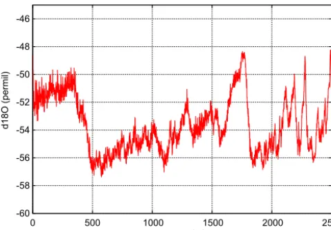
Figure 1.δ18O data used in this study.

from the shallow ice approximation (SIA) and is based on a linearization of the temperature profile. Martin and Gud-mundsson (2012) have shown that the Lliboutry equation is not appropriate for a steady dome. However, we can expect that the domes in central Antarctica are non-steady because the Raymond bumps have never been observed. We thus as-sume that the Lliboutry equation can still be used. Denoting the melting rate at the base of the ice sheet as m,Aandm

correspond to the vertical velocity atζ =1 and that atζ =0, respectively, under a pseudo-steady state. Equation (6) can thus be rewritten as follows:

u(ζ )= −1 H

m+(A−m) ω(ζ )

. (8)

Settingµ=m/(A−m), Eqs. (5) and (8) yield

2(ζ )=ω(ζ )+µ

1+µ . (9)

We assumeµis constant, which means the ratiom / Ais con-stant. This assumption would be approximately justified be-causemis typically much smaller thanA. Using Eqs. (7) and (9), the thinning factor2can be determined if the parameters

s,p, andµare specified.

In order to obtain the ageξ using Eq. (2), it is also nec-essary to give the profile of the accumulation rateA. In this study,Ais treated as an unknown to be estimated. Since the accumulation rate is related to the Antarctic temperature, we can use proxies of the temperature for constraints when es-timating the profile of A. As a proxy for the temperature, we used theδ18O data taken at Dome Fuji (Watanabe et al., 2003), which are plotted in Fig. 1. Since the vertical profile of the ageξ is associated with the profile ofA, the informa-tion from the δ18O data is also effective for improving the estimate of the ageξ.

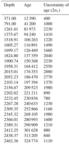
At several depths, we can also use reliable age values given by age markers. We used such age values as tie points when estimating the age–depth relationship. The age, depth, and

uncertainty (2σ) for each tie point used in the paper are shown in Table 1. The first point was determined from the Antarctic Cold Reversal to Holocene transition and the sec-ond one was determined from the beryllium 10 peak. These two points were given by Parrenin et al. (2007). The subse-quent 23 points were determined from the relationship be-tween O2/N2and the summer insolation (Kawamura et al., 2007). Both theδ18O data and the tie points were considered when estimating the ageξ.

3 State space model

In this section, the age–depth relationship is formulated in a framework of a state space model on the basis of the model described in the previous section. The state space model rep-resents the evolution of variables by a recurrence equation. The state space model provides a platform for the sequential Bayesian estimation using PMCMC, which will be explained in the next section.

Discretizing the vertical coordinatezwith an interval1z, the integral in Eq. (2) for any discretizedzcan be approxi-mately calculated using the following recurrence relation:

ξz+1z≈ξz+

1z Az2z

(z=0, 1z,21z, . . ., Z−1z), (10) whereξzdenotes the age at depthz, and we denote the accu-mulation rate and the thinning factor in the interval fromzto

z+1zbyAzand2z, respectively. At the surface (z=0),ξ0 is defined as 0. The depth at the bottom of the core is denoted byZ.

Equation (10) would contain an error due to the discretiza-tion of Eq. (2). In addidiscretiza-tion, since we can not accurately know

Azand2zfor eachz, an estimate of the age–depth relation-ship might also be affected by errors inAz and2z. We rep-resent these unspecified errors byνz. Equation (10) is thus modified as follows:

ξz+1z=ξz+

1z Az2z

+νz

s 1z Az2z

(z=0, 1z,21z, . . ., Z−1z). (11)

We assume thatνzobeys the normal distributionsN(0, σν2), where we denote a normal distribution with meanµand vari-anceσ2byN(µ, σ2). We multiply νzby

p

1z / (Az2z)in order that the variance of the unknown variation per year re-main the same to the bottom of the core. In a pseudo-steady state, the thinning factor 2z can be obtained according to Eq. (9). However, Eq. (9) does not consider all of the effects governing the thinning process2z; for example, it omits the effect of impurities (Freitag et al., 2013). The errors in2due to such unspecified effects would also be considered byνzin Eq. (11).

(4)

Table 1. Depth, age, and uncertainty of age at each tie point.

Depth Age Uncertainty of age (2σε)

371.00 12 390 400 791.00 41 200 1000 1261.61 81 973 2230 1375.67 94 240 1410 1518.91 106 263 1220 1605.27 116 891 1490 1699.17 126 469 1660 1824.80 137 359 2040 1900.74 150 368 2230 1958.31 164 412 2550 2015.01 176 353 2880 2052.23 186 470 2770 2103.14 197 394 1370 2156.67 209 523 1980 2202.02 221 211 890 2232.45 230 836 780 2267.28 240 633 1230 2309.35 252 866 1160 2345.32 268 105 1980 2366.01 280 993 1600 2389.31 290 909 1210 2412.25 301 628 880 2438.37 313 205 840 2462.36 324 774 1110 2505.4 343 673 2000

following recurrence relation:

logAz+1z=logAz+ηz

s 1z Az2z

(z=0, 1z,21z, . . ., Z−1z). (12)

Note that in Eq. (12), the transition of Az is described by using its logarithm in order to guaranteeAz>0. The termηz represents the (unknown) variation in the accumulation rate. We assume thatηz obeysN(0, ση2). We hereinafter assume

1z=1[m]. Equations (11) and (12) can thus be rewritten as follows:

ξz+1=ξz+ 1

Az2z

+√νz Az2z

, (z=0, . . ., Z−1) (13) logAz+1=logAz+

ηz

√ Az2z

, (z=0, . . ., Z−1). (14)

Based on Eqs. (13) and (14), we introduce conditional probability density functions. Since we assumed νz andηz obeyN(0, σ_ν2)andN(0, σ_η2), respectively, the conditional distribution ofξz+1givenξz and that ofAz+1givenAzfor

eachzbecome

p(ξz+1|ξz,θ)=N

ξz+

1

Az2z

, σ

2 ν

Az2z

and (15)

p(Az+1|Az,θ)=logN Az,

σ_η2

Az2z

!

, (16)

respectively, whereθindicates a collection of unspecified pa-rameters such aspandsin Eq. (7). The full definition ofθ will be provided later.

Estimates ofξzandAzfor eachzare obtained on the basis of their posterior distributions given the tie points and the

δ18O data. For thekth tie pointτkat depthzk, we assume the following relationship betweenτk and the modeled ageξzk:

τk=ξzk+εk, (17)

whereεk is the discrepancy between the age at the tie point and the modeled age. We assume thatεk obeys the normal distributionN(0, σ_ε2). While we consider the uncertainty in the age of tie points, we assume there to be no uncertainty in the depths of tie points. This is because the depth uncertainty would not have essential effects on the estimate of the age for each slice of the ice core. The effects of the depth uncer-tainty on the estimates of accumulation and thinning are also expected to be minor, because the accumulation and thinning are related to the increment of depth rather than the absolute depth from the surface. In this study, the uncertainty in the age increment is taken into account byνz in Eq. (13). This would compensate for the possible effect of the depth un-certainty on the estimates of accumulation rate and thinning factor.

Theδ18O data, which are associated with the accumulation rate, can be abundantly obtained from the ice core at Dome Fuji. Multiple data points forδ18O are sometimes available within an interval of a single meter, and we used the mean

δ18O value for each such interval. It was assumed thatAz, the accumulation rate in the interval fromztoz+1, is associated withδ18O as follows:

δ18Oz=alogAz+b+wz; (18)

this relation was also used by Klauenberg et al. (2011). We assume thatwz obeys the normal distributionN(0, σw2). Al-though we assume the regression coefficientsaandbdo not depend on age, it is not guaranteed that the accumulation rate andδ18O have the same linear relationship over the entire period recorded in the ice core. Even if we could accept the linear assumption between the accumulation rate andδ18O,

(5)

between the accumulation rate andδ18O would be absorbed byηz.

Like Eqs. (15) and (16), we introduce conditional proba-bility density functions based on Eqs. (17) and (18). Since we assumed εz andwz obeyN(0, σε2)andN(0, σw2), respec-tively, the conditional distribution ofτk givenξzk and that of δ18OzgivenAzbecome

p(τk|ξzk,θ)=N

ξzk, σ

2 ε

, (19)

p(δ18Oz|Az,θ)=N

alogAz+b, σw2

. (20)

We hereinafter combine ξz and Az into one vector xz asxz=(ξz Az)T. Becausep(ξz+1|ξz,θ)andp(Az+1|Az,θ) are given, the joint distribution p(ξz+1, Az+1|ξz, Az,θ)can also be defined. Thus,

p(xz+1|xz,θ)=p(ξz+1, Az+1|ξz, Az,θ). (21) We also define the vector of the available data for eachzas y_z. If both the tie pointτkz and theδ

18_{O data are available} atz, theny_z=(τkz, δ

18_Oz₎T_{. If the}_δ18_{O data are available} but a tie point is unavailable, we definey_z=δ18Oz. If nei-ther a tie point nor δ18O data are available, we definey_z=

Ø. Usingy_z, the conditional distributions in Eqs. (19) and (20) can then be combined into the conditional distribution

p(y_z|xz,θ)for anyz, where we definep(yz=Ø|xz,θ)=1. Our aim is to estimatex0:Z= {x0, . . .,xZ}based on the se-quence of the datay₁:Z= {y1, . . .,yZ}. If a set of the param-etersθwere given, we could obtain an estimate ofx0:Zfrom the posterior distributionp(x0:Z|y1:Z,θ). However, since the value ofθis not specified, it is necessary to take into account the uncertainties of θ in estimating x0:Z. We obtain an es-timate from the marginal posterior distribution given y₁:Z, whereθis marginalized out:

p(x0:Z|y1:Z)=

Z

p(x0:Z|y1:Z,θ) p(θ|y1:Z)dθ. (22) Sincey_z is conditionally independent ofxz0 givenx_z when z06=z,

p(y_z|x0:z,θ)=p(yz|xz,θ). (23) Hence, p(x0:Z|y1:Z,θ) satisfies the following recurrence equation:

p(x0:z|y1:z,θ)

∝p(y_z|xz,θ) p(x0:z|y1:z−1,θ)

=p(y_z|xz,θ) p(xz|xz−1,θ) p(x0:z−1|y1:z−1,θ). (24) By applying Eq. (24) recursively, we can obtain

p(x0:z|y1:z,θ)for anyz. Thus, sampling fromp(x0:z|y1:z,θ) can be achieved using the sequential Monte Carlo (SMC) method (Doucet et al., 2001; Liu, 2001). If zin Eq. (24) is set at the depth at the bottom of the ice core (i.e.,z=Z), we

obtain p(x0:Z|y1:Z,θ), which provides the estimate of the age given all the data for the entire ice core.

We can also estimate the parameterθ. The posterior dis-tribution ofθ giveny₁_:_Z in Eq. (22) is calculated using the following equation:

p(θ|y₁_:_Z)∝p(y₁_:_Z|θ) p(θ). (25) The vectorθcontains all of the unspecified parameters used above. The full definition ofθis as follows:

θ= A0a b µ p s σν σησw T

. (26)

An approximation ofp(y₁_:_Z|θ)can be calculated using the SMC method. Therefore, if the priorp(θ)is given, the pos-terior ofθcan readily be obtained. In this study, we use flat prior distributions. Since it is unreasonable to allow the pa-rameters exceptaandbto be negative, the prior distributions for these non-negative parameters were assumed to be a uni-form distribution on the non-negative real line. The prior dis-tributions for the other parametersaandbwere assumed to be a uniform distribution on the real line. The shape of the posterior thus corresponds to that of the likelihood function in this study.

Since the present accumulationA0is not specified in the above sequential model,A0is treated as one of the unspec-ified parameters and is included in θ. The parameter vec-torθ also contains three hyper-parameters σν,ση, andσw, which represent the variabilities in the model. These hyper-parameters are estimated so as to well explain the variability observed in the data. For example, ifσν is taken to be too small, the estimated age would not fit the data well. On the other hand, ifσν is taken to be too large, large variations in the ageξ are allowed. Thus, the result could be sensitive to the noise contained in the data. The posterior given the data provides an appropriate value ofσν so that it is large enough to achieve a good fit, but not too large. The posterior ofσw indicates the typical magnitude of dispersion of δ18O data from the predictedδ18O based on the estimated accumula-tion rate. We did not includeσεinθ, but we set a fixed value forσεfor each tie point, as shown in Table 1; the values were determined according to Kawamura et al. (2007).

4 Estimation algorithm

In order to approximate the conditional distributions

(6)

The SMC method can be used to obtainp(x0:Z|y1:Z, θ ) un-der a given θ, but it can not be used to obtain p(θ|y1:Z). In principle, MCMC could be used to obtain any proba-bility distribution, includingp(x0:Z|y1:Z, θ ),p(θ|y1:Z), and

p(x0:Z|y1:Z). However, this would require prohibitive com-putational cost for high-dimensional problems. Thus, use of MCMC is not practical for obtaining high-dimensional distri-butions likep(x0:Z|y1:Z, θ )andp(x0:Z|y1:Z). By combining SMC and MCMC, we can obtainp(x0:Z|y1:Z, θ ),p(θ|y1:Z), and p(x0:Z|y1:Z) with an acceptable computational cost. Below, we first present the SMC method on which the PMCMC method is based. We then describe the PMCMC method and explain how approximations ofp(x0:Z|y1:Z,θ) andp(θ|y₁_:_Z)can be obtained.

4.1 Sequential Monte Carlo method

The SMC method, which is sometimes referred to as the par-ticle filter/smoother in time-series analysis (Gordon et al., 1993; Kitagawa, 1996; Doucet et al., 2001), is used for sampling from the conditional distribution p(x0:Z|y1:Z,θ). The SMC method approximates a probability distribution by a set of N particles, which are the samples drawn from the distribution. Letx(i)₀_:_z₋₁_|_z₋₁be theith sample from

p(x0:z−1|y1:z−1,θ); we have the following approximation:

p(x0:z−1|y1:z−1,θ)≈ 1

N

X

i=1

δx0:z−1−x(i)₀:z−1|z−1

, (27)

where δ(·)denotes the Dirac delta function. If we draw a particlex(i)_z_|_z₋₁for eachiaccording to

x(i)_z_|_z₋₁∼pxz|xz−1=x(i)z−1|z−1,θ

, (28)

then the set of particles{x(i)₀_:_z_|_z₋₁}provides an approximation ofp(x0:z|y1:z−1,θ):

p(x0:z|y1:z−1,θ)≈ 1

N

X

i=1

δx0:z−x(i)0:z|z−1

. (29)

An approximation of the distribution conditioned by the ob-servationy_zatzcan be obtained using the importance sam-pling scheme (e.g., Liu, 2001; Robert and Casella, 2004):

p(x0:z|y1:z,θ)=

p(y_z|x_z,θ) p(x0:z|y1:z−1,θ)

p(y_z|y₁:z−1,θ)

≈

N

X

i=1

β_z(i)δx0:z−x(i)₀:z|z−1

. (30)

The weightβz(i)for eachiis defined as

β_z(i)=

py_z|x(i)_z_|_z₋₁,θ

PN

i=1p

y_z|x(i)_z_|_z₋₁,θ

, (31)

wherep(y_z|x(i)_z_|_z₋₁,θ)is called the likelihood of the particle x(i)_z_|_z₋₁.

Equation (30) indicates thatp(x0:z|y1:z,θ)can be approx-imated by weighting the particles {x(i)₀_:_z_|_z₋₁}. However, the weights are usually highly unbalanced and many of the par-ticles have only negligible weights. Because parpar-ticles with negligible weights no longer contribute to the estimation, this destroys the efficiency of the approximation. In order to re-solve the imbalance in the weights, a new set ofN parti-cles{x(i)₀_:_z_|_z}is obtained by resampling the original particles

{x(i)₀_:_z_|_z₋₁}such that eachx(i)₀_:_z_|_z₋₁is drawn with a probability ofβz(i) (see Nakano et al., 2007; van Leeuwen, 2009). Af-ter resampling, the original particles in{x(i)₀_:_z_|_z₋₁}that have low weights are removed, and those that have high weights are duplicated. The number of the duplicates ofx(i)₀_:_z_|_z₋₁,n(i)z , becomes approximately equal toN βz(i). The newly generated particles then provide an approximation ofp(x0:z|y1:z,θ)as follows:

p(x0:z|y1:z,θ)≈ N

X

i=1

β_z(i)δx0:z−x(i)₀:z|z−1

≈

N

X

i=1

n(i)z

N δ

x0:z−x(i)0:z|z−1

= 1 N

N

X

i=1

δx0:z−x(i)₀:z|z

. (32)

Applying the procedure from Eqs. (27) to (32) recursively up toz=Z, we obtain samples from the conditional dis-tribution p(x0:Z|y1:Z,θ). If only the marginal distribution

p(xz|y1:z,θ), wherex0:z−1is marginalized out, is of inter-est, it is not necessary to keep the whole sequence ofx(i)₀_:_z_|_z for each particle; instead, at each iteration, it is sufficient to keep only the elementx(i)_z_|_zand discard the remainingx(i)₁_:_z₋₁. 4.2 Particle Markov chain Monte Carlo method An approximation of the marginal likelihood p(y₁_:_Z|θ)in Eq. (25) can be calculated using SMC (Kitagawa, 1996). If we decomposep(y₁_:_Z|θ)as

p(y₁_:_Z|θ)=p(y₁_:_Z₋₁|θ) p(y_Z|y₁_:_Z₋₁,θ)

=p(y₁|θ)

Z

Y

z=2

p(y_z|y₁_:_z₋₁,θ), (33) we can obtainp(y_z|y₁_:_z₋₁,θ)for eachz, from the following equation:

p(y_z|y₁:z−1,θ)

= Z

(7)

Eq. (34) can be obtained as follows:

p(y_z|y₁_:_z₋₁,θ)

≈ 1 N

N

X

i=1

Z

p(y_z|xz,θ) δ

x0:z−x(i)₀:z|z−1

dx0:z

= 1 N

N

X

i=1

p(y_z|x(i)₀_:_z_|_z₋₁,θ), (35)

where we used Eq. (23). We can then approximate the loga-rithm ofp(y₁_:_Z|θ):

logp(ˆ y₁_:_Z|θ)=

Z

X

z=1 log

"

1

N

X

i=1

p(y_z|x(i)₀_:_z_|_z₋₁,θ) #

, (36)

and an approximation of the posteriorp(θ|y₁:Z)in Eq. (25) can accordingly be obtained. As a matter of fact, however, the approximation given in Eq. (36) for the log likelihood is too sensitive to the parameterθbecause of the large amount ofδ18O data. We thus introduce the following relaxation:

logp(ˆ y₁:Z|θ)= Z

X

z=1 log

"

1

N

X

i=1

pδ18Oz|x₀(i):z|z−1,θ

λ pτkz|x

(i) 0:z|z−1,θ

#

, (37)

where we set λ=1/5 so that the information of tie points becomes effective enough.

Using the Monte Carlo approximation of the marginal likelihoodp(ˆ y₁:Z|θ), we can obtain an approximation of the marginal posterior distribution ofθusing MCMC, which se-quentially produces samples that obey the target distribution. This is the basic idea of the PMCMC method. There are some variants of the PMCMC method such as the particle Gibbs method with ancestor sampling (Lindsten et al., 2014). In this study, because of the ease of implementation, we employ the Metropolis method to obtain an approximation ofp(θ|y₁_:_Z). In the Metropolis method, at the kth iteration, a proposal sample θ∗ is drawn from the proposal density q(θ|θ(k−1)), which is conditioned by the sample θ(k−1) obtained at the previous iteration:

θ∗∼q(θ|θ(k−1)). (38)

In this paper, the proposal distribution q was taken to be a zero-mean Gaussian distribution with a fixed variance for each element ofθ. This means we assume a symmetrical pro-posal distribution satisfying

q(θ|θ0)=q(θ0|θ) (39)

for anyθandθ0. The variance ofq(θ|θ0)was tuned by pre-liminary runs. In obtaining the final results, the variances were set at 0.05,0.1,0.1,0.001,0.2,0.01,5.0,0.0002, and

0.005 for the parametersA0, a, b, µ, p, s, σν, ση, andσw, re-spectively, in order that the Markov chain rapidly moves around in the parameter space. The proposal sample θ∗ is accepted with the following probability:

min 1, p(ˆ y1:Z|θ ∗

) p(θ∗)

ˆ

p(y₁_:_Z|θ(k−1)) p(θ(k−1)) !

, (40)

wherep(ˆ y₁_:_Z|θ)is an approximation of the marginal like-lihood obtained by SMC as written in Eq. (37). If θ∗ is accepted, we setθ(k)=θ∗; otherwise, we setθ(k)=θ(k−1) and thusp(ˆ y₁:Z|θ(k))= ˆp(y1:Z|θ(k−1)). Usingθ(k), the pro-posal sample at the next iteration can be obtained accord-ing to Eq. (38). Iterataccord-ing the above procedure generates a large number of samples that obey the posterior distribution

p(θ|y₁:Z). A short summary of PMCMC is also found in a pseudo-code in the original paper by Andrieu et al. (2010).

In the above algorithm, an approximated value of the marginal likelihoodp(y₁_:_Z|θ)is computed using the SMC method at each iteration of the Metropolis method. It should be noted that Eq. (34) can be modified as follows:

p(y_z|y₁_:_z₋₁,θ)= Z

p(y_z|xz,θ) p(xz|xz−1,θ)

·p(xz−1|y1:z−1,θ)dxz−1dxz. (41) Thus, in calculatingp(y₁:Z|θ)in Eq. (33), it is not necessary to consider the joint distribution of the sequencex0:Z; it is sufficient to consider the marginal distributionp(xz|y1:z,θ) for eachz. As mentioned above, sampling fromp(x_z|y₁_:_z,θ)

can be achieved when discarding x1:z−1. This greatly re-duces the computational cost because it can skip some pro-cedures for handling the whole sequence of 2510 time steps (Z=2510 in this paper) for 5000 particles. In addition, the memory cost is also remarkably reduced, although the mem-ory cost could be reduced by using another efficient algo-rithm by Jacob et al. (2015). We then discardx1:z−1in order to obtain an approximation ofp(y₁:Z|θ)at each iteration of the Metropolis method.

As mentioned in Sect. 3, if we retain the samples for the whole sequencex0:Z from a run of SMC with a given θ, we obtain samples from p(x0:Z|y1:Z,θ). The Metropo-lis procedure sequentially generates a large number of sam-ples that obey the marginal posterior distributionp(θ|y₁:Z). By combining the SMC samples with variousθ values that obey p(θ|y₁_:_Z), we can obtain the samples representing the marginal posterior distributionp(x0:Z|y1:Z)whereθ is marginalized out according to Eq. (22). If samples that obey

(8)

5 Results

We applied the PMCMC method to the Dome Fuji ice core. In this study, the thickness of the ice sheet H is assumed to be 3031 m. The bottom of the core Z is 2505 m. Fol-lowing a burn-in period, we performed 250 000 iterations of the Metropolis sampling, and we retained a sample ev-ery fifth iteration. We thus drew 50 000 samples from the marginal posterior distribution ofθ,p(θ|y₁:Z). For each run of SMC, 5000 particles were used to obtain samples from

p(x0:Z|y1:Z,θ(k)).

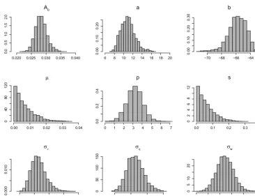
Figure 2 shows the marginal histograms for the esti-mated posterior distribution for each parameter. The poste-rior mean and standard deviation of the present accumula-tion rateA0(=A(0))were 0.0278 and 0.0019 (m yr−1), re-spectively. This result is in good agreement with the mea-surements by Kameda et al. (2008), who reported the surface mass balance at Dome Fuji to be 27.3±1.5 kg(m−2_yr−1₎_, which corresponds to about 0.0273 m yr−1. The maxima of the posterior distributions forµands were estimated to be near 0. This result is similar to that obtained in a previous study that used the Metropolis-Hastings method (Parrenin et al., 2007). The result in Fig. 2 suggests thatµis most likely between 0 and 2 % of the accumulation rate. Considering that the accumulation rate A was mostly less than 0.03 m yr−1, we can guess that the basal melting rate is mostly less than 0.0006 m yr−1(=0.6mm yr−1). This roughly agrees with the result by Parrenin et al., who showed that the basal melt-ing rate is likely to be less than 0.4mm yr−1. Such a small value ofmis consistent with our assumption of the pseudo-steady state, in which the ratiom/Ais constant as described in Sect. 2. In the result by Parrenin et al. (2007), the posterior ofppeaks around 3, and another peak was suggested around

p=2. On the other hand, the results obtained in this study suggest that the posterior ofp peaks around 3, and it is not clear whether there is another mode. It should be noted that these two results were based on different models of the accu-mulation rate. In addition, the setting of the thinning factor in this study is different from that used by Parrenin et al. as dis-cussed later. Thus, it should not be expected that they would necessarily provide similar results.

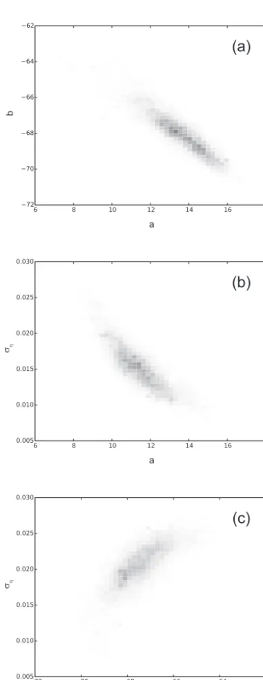
In the posterior distribution, some of the parameters are correlated with each other. Figure 3 shows two-dimensional histograms of the marginal posterior distribution ofa andb

(a), the marginal posterior distribution ofa andση(b), and the marginal posterior distribution ofbandση(c). Close cor-relations between the three parameters a,b, andση are ob-served in this posterior distribution. These three parameters are related to the accumulation rate andδ18O data. Thus, the accuracy of the estimation for these three parameters could be much improved if any of the three parameters could be effectively constrained.

Figure 4 shows the estimated age as a function of depth. The red solid line indicates the median of the posterior dis-tribution and the red dotted lines indicate the 10th and 90th

percentiles of the posterior distribution. For reference, the re-sult by Parrenin et al. (2007) is indicated by a grey line. The black crosses in this figure indicate the tie points used for the estimation. In order to verify the convergence of the SMC sampling, we repeated sampling from the marginal posterior distributionp(x0:Z|y1:Z)five times with different seeds and confirmed that there were no apparent differences between the results of the five trials. (The figures shown in this paper show the result of one of the five trials.) Thus, the estimate shown in Fig. 4 is considered reliable. The SMC method of-ten suffers from the degeneracy problem, especially when the number of steps is large. In PMCMC, this problem is over-come by collecting a large number of SMC samples from the iterations of the Metropolis method. In Fig. 4, it is difficult to discriminate the 10th and 90th percentiles from the me-dian because the width of the posterior distribution is much smaller than the range of Fig. 4. In order to make the width of the posterior visible, the 10th and 90th percentiles of the pos-terior distribution are indicated by red dotted lines around the median of the posterior distribution in Fig. 5. Black crosses show the difference between each tie point and the median of the posterior. The uncertainty of age is minimized at each tie point, where the age is known with high accuracy, although it is not possible to completely remove any uncertainty. In Fig. 5, a grey line indicates the difference between the esti-mate by Parrenin et al. (2007) and the median of the posterior obtained by the proposed method. Note that this line tends to deviate further from the median than do the black crosses. This means that the estimate with the proposed method fits the tie points more closely than does the estimate by Parrenin et al., although the difference between the two results is about 3000 years at the greatest.

(9)

0.

0

0.5

1.

0

1.5

2.

0

6 8 10 12 14 16 18 20

0.00

0.10

0.20

−70 −68 −66 −64

0.00

0.10

0.20

0.30

0.00 0.01 0.02 0.03 0.04

0

40

80

120

0 1 2 3 4 5 6 7

0.

0

0.2

0.

4

0.0 0.1 0.2 0.3 0.4

02468

12

50 100 150 200 250

0.000

0.010

0.010 0.015 0.020 0.025

0

50

100

150

0.30 0.32 0.34 0.36 0.38 0.40

0

5

10

20

A₀ a b

p s

μ

σν ση σw

0.020 0.025 0.030 0.035 0.040

Figure 2. Estimated marginal distributions of the posterior distributions for the nine parameters.

shown in Fig. 7, we have the posterior distribution of the ac-cumulation rate given depthp(A|z). The accumulation rate with respect to age is estimated after considering the uncer-tainty of age:

p(A|ξ )= Z

p(A|z) p(z|ξ )dz (42)

where we assumep(z)to be a uniform distribution when ob-tainingp(z|ξ ):

p(z|ξ )=_R p(ξ|z)p(z)

p(ξ|z)p(z)dz. (43)

Figure 8 shows the estimate of the accumulation rate with respect to age.

6 Discussion

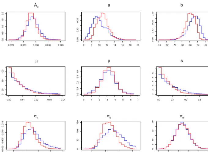
In order to evaluate the robustness, we obtained the estimate without using the last five tie points at below 2400 m depth. We estimated the parameters and the age–depth relationship from the other 20 tie points and theδ18O data. Figure 9 shows the histograms of the marginal posterior distributions of the nine parameters. The results without using the five tie points are indicated by blue lines and the results with all the tie points, which are the same as the results in Fig. 2, are indi-cated as red lines. The posterior distributions obtained with-out some of the tie points are very similar to the result shown

in Fig. 2. However, the posterior distributions of the three parametersa,b, andση are slightly different. Sinceση was estimated to be larger when the five tie points were not used, this might indicate that the variation in the accumulation rate was noisier near the bottom. The marginal posterior distri-bution fora andbcould accordingly be modified due to the correlation withσηshown in Fig. 3. However, more careful evaluation would be required to determine the reason.

Figure 10 shows the estimates of the age as a function of depth are compared between the result without using the last five tie points and that with all the tie points. In order to make the differences visible, this figure shows the differences from the median of the posterior without the last five tie points like in Fig. 5. The red lines indicate the estimate without the last five tie points, and the grey lines indicate the estimate with all the tie points. The dotted lines indicate the 10th and 90th percentiles of the posterior distributions. The tie points used for the estimation are shown with black crosses. The devia-tion of the grey lines tended to be large near the bottom of the ice core. However, the grey lines were within the range of un-certainty shown with the red dotted lines. This suggests that our model does a good job of representing the uncertainties due to the lack of the information.

(10)

ση

a

(b)

a

b

(a)

b ση

(c)

Figure 3. Two-dimensional histograms of the marginal posterior

distribution ofaandb(a), the marginal distribution ofa andση

(b), and the marginal distribution ofbandση(c).

line indicates the estimate using all the tie points. The solid lines indicate the median of the posterior, and the 10th and 90th percentiles are indicated by dotted lines. The difference is remarkable below the depth where the age is 300 000 years. However, the difference was mostly within the uncertainty between the 10th and 90th percentiles. Thus, this difference near the bottom is acceptable.

The proposed technique requires a high computational cost because the SMC sampling is performed at each

itera-0 500 1000 1500 2000 2500

0

50000

150000

250000

350000

Ag

e

Depth (m)

Figure 4. Estimated age as a function of depth. The solid line

in-dicates the median of the posterior distribution. The 10th and 90th percentiles of the posterior are indicated by red dotted lines. The black crosses indicate the tie points. The result obtained by Parrenin et al. (2007) is also indicated by a grey line.

0 500 1000 1500 2000 2500

−4000

−2000

0

2000

4000

Depth (m)

Difference in age

Figure 5. Difference of the 10th and 90th percentiles of the

poste-rior distribution from the median of the posteposte-rior (red dotted lines), difference of each tie point from the median of the posterior (black crosses), and difference of the estimate by Parrenin et al. (2007) from the median of the posterior obtained in this study (grey line).

tion of the Metropolis method. At present, it takes about 43 h to complete 250 000 iterations of the Metropolis sampling with 5000 particles for the SMC on a workstation with two Intel Xeon processors (12 cores for each processor; 2.7 GHz). The efficiency could be improved by using a better proposal distribution used in SMC (e.g., Doucet et al., 2001). This problem should be addressed in the future.

(11)

0 500 1000 1500 2000 2500

0.0

0.2

0.4

0.6

0.8

1.0

Depth (m)

Thinning

Figure 6. Estimated thinning factor2as a function of depth. The median of the posterior is indicated by a red solid line, the 10th and 90th percentiles are indicated by red dotted lines, and the estimate by Parrenin et al. (2007) is indicated by a grey line.

0 500 1000 1500 2000 2500

012345

Depth (m)

Accumulation rate

2

10 [− m-of-ice/year] ×

Figure 7. Estimated accumulation rate as a function of depth. The

median of the posterior is indicated by a red solid line, the 10th and 90th percentiles are indicated by red dotted lines, the difference between the 10th and 90th percentiles is indicated by a blue dotted line, and the estimate by Parrenin et al. (2007) is indicated by a grey line.

the transition and another distribution for the perturbation. There are a large number of choices for the model for the accumulation rate, and the goodness of fit could be evalu-ated using some metric such as Bayes factors. However, it would require a great deal of time to evaluate a wide variety of choices, and so such a search is beyond the scope of this study.

This study used theδ18O data and tie points deduced from O2/N2 data to estimate the age–depth relationships. How-ever, PMCMC allows us to use various kinds of data. Thus, data from other various sources could also be used to improve the accuracy of the estimates. For example, deuterium-excess

0 50000 100000 150000 200000 250000 300000 350000

012345

Age

Accumulation rate

2

10 [− m-of-ice/year] ×

Figure 8. Estimated accumulation rate as a function of age. The

median of the posterior is indicated by a red solid line, the 10th and 90th percentiles are indicated by red dotted lines, the difference between the 10th and 90th percentiles is indicated by a blue dotted line, and the estimate by Parrenin et al. (2007) is indicated by a grey line.

data have been used to estimate temperatures (Uemura et al., 2012), and this could be used for improving the accuracy of the accumulation rate. Some recent studies have provided simultaneous estimates of the age as a function of depth at multiple sites (e.g., Lemieux-Dudon et al., 2010; Veres et al., 2013). The SMC approach could be extended to include in-formation at multiple sites; this would be a useful area for future work.

7 Concluding remarks

(12)

0.

0

0.5

1.

0

1.5

2.

0

6 8 10 12 14 16 18 20

0.00

0.10

0.20

−74 −72 −70 −68 −66 −64 −62 −60

0.00

0.10

0.20

0.30

0.00 0.01 0.02 0.03 0.04

0

20

60

100

0 1 2 3 4 5 6 7

0.

0

0.1

0.

2

0.3

0.

4

0.0 0.1 0.2 0.3 0.4

0246

8

10

50 100 150 200 250

0.000

0.005

0.010

0.015

0.010 0.015 0.020 0.025

0

50

100

150

0.30 0.32 0.34 0.36 0.38 0.40

0

5

10

20

30

A₀ a b

p s

μ

σ_ν σ_η σ_w

0.020 0.025 0.030 0.035 0.040

Figure 9. Estimated marginal distributions of each of the nine parameters: without using the last five tie points (blue) and with all the tie

points (red).

0 500 1000 1500 2000 2500

−6000

−4000

−2000

0

2000

4000

6000

Depth (m)

D

iff

er

en

ce

i n

a

ge

Figure 10. Difference of the 10th and 90th percentiles of the

poste-rior distribution from the median of the posteposte-rior (red dotted lines) for the result without using the last five age markers. The difference of each tie point from the median of the posterior (black crosses) and the difference between the estimate with all the tie points and the estimate without using the last five tie points (grey line) are also shown.

The main advantage of the proposed technique is that it can be applied to general nonlinear non-Gaussian situations. Since the relationship between accumulation rate and a tem-perature proxy is typically nonlinear, it is not necessarily justified to assume linearity and Gaussianity when using a temperature proxy to date an ice core. The PMCMC method allows us to use various kinds of data that are expected to have a nonlinear relationship with the model variables.

An-0 50000 100000 150000 200000 250000 300000 350000

0

1

2345

Age

Accumulation rate

2

10 [− m-of-ice/year]

×

Figure 11. Estimated accumulation rate as a function of age:

with-out using the last five tie points (red) and with all the tie points (grey). The solid lines indicate the median of the posterior distribu-tion. The 10th and 90th percentiles of the posterior are indicated by dotted lines.

(13)

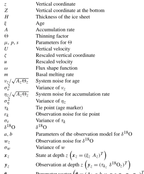
Appendix A

Table A1. Definition of the variables used in this paper.

z Vertical coordinate

Z Vertical coordinate at the bottom

H Thickness of the ice sheet

ξ Age

A Accumulation rate

2 Thinning factor

µ,p,s Parameters for2

U Vertical velocity

ζ Rescaled vertical coordinate

u Rescaled velocity

ω Flux shape function

m Basal melting rate

νz/

√

Az2z System noise for age

σ_ν2 Variance ofνz

ηz/

√

Az2z System noise for accumulation rate

σ_η2 Variance ofηz

τk Tie point (age marker)

εk Observation noise for tie point

σε Variance ofτk

δ18O δ18O

a,b Parameters of the observation model forδ18O

wz Observation noise forδ18O

σw Variance ofw

xz State at depthz

xz=(ξzAz)T

yz Observation at depthz

yz=(τkzδ18Oz)T

θ Parameter vectorθ=(A0a b µ p s σνσησw)T

(14)

Acknowledgements. This work was conducted under project

“Exploration for Seeds of Integrated Research”, supported by the Transdisciplinary Research Integration Center, Research Organization of Information and Systems.

Edited by: A. M. Mancho

Reviewed by: M. Winstrup and two anonymous referees

References

Andrieu, C., Doucet, A., and Holenstein, R.: Particle Markov chain Monte Carlo methods, J. Roy. Statist. Soc. B, 72, 269–342, 2010. Doucet, A., de Freitas, N., and Gordon, N. (Eds.): Sequential Monte

Carlo methods in practice, Springer-Verlag, New York, 2001. Dreyfus, G. B., Parrenin, F., Lemieux-Dudon, B., Durand, G.,

Masson-Delmotte, V., Jouzel, J., Barnola, J.-M., Panno, L., Spahni, R., Tisserand, A., Siegenthaler, U., and Leuenberger, M.: Anomalous flow below 2700 m in the EPICA Dome C ice core detected using d18O of atmospheric oxygen measurements, Clim. Past, 3, 341–353, doi:10.5194/cp-3-341-2007, 2007. Freitag, J., Kipfstuhl, S., and Laepple, T.: Core-scale radioscopic

imaging: a new method reveals density–calcium link in Antarctic firn, J. Glaciology, 59, 1009–1014, doi:10.3189/2013JoG13J028, 2013.

Gordon, N. J., Salmond, D. J., and Smith, A. F. M.: Novel approach to nonlinear/non-Gaussian Bayesian state estimation, IEE Pro-ceedings F, 140, 107–113, 1993.

Jacob, P. E., Murray, L. W., and Rubenthaler, S.: Path storage in the particle filter, Stat. Comput., 25, 487–496, 2015.

Kameda, T., Motoyama, H., Fujita, S., and Takahashi, S.: Temporal and spatial variability of surface mass balance at Dome Fuji, East Antarctica, by the stake method from 1995 to 2006, J. Glaciol., 54, 107–116, 2008.

Kawamura, K., Parrenin, F., Lisiecki, L., Uemura, R., Vimeux, F., Severinghaus, J. P., Hutterli, M. A., Nakazawa, T., Aoki, S., Jouzel, J., Raymo, M. E., Matsumoto, K., Nakata, H., Mo-toyama, H., Fujita, S., Goto-Azuma, K., Fujii, Y., and Watan-abe, O.: Northern Hemisphere forcing of climatic cycles in Antarctica over the past 360,000 years, Nature, 448, 912–916, doi:10.1038/nature06015, 2007.

Kitagawa, G.: Monte Carlo filter and smoother for non-Gaussian nonlinear state space models, J. Comp. Graph. Statist., 5, 1–25, 1996.

Klauenberg, K., Blackwell, P. G., Buck, C. E., Mulvaney, R., Röth-lisberger, R., and Wolff, E. W.: Bayesian glaciological modelling to quantify uncertainties in ice core chronologies, Quat. Sci. Rev., 30, 2961–2975, 2011.

Lemieux-Dudon, B., Parrenin, F., and Blayo, E.: A probabilistic method to construct an optimal ice core chronology for ice cores, in: Proceedings of the 2nd International Workshop on Physics of Ice Core Records (PICR-2), edited by: Hondoh, T., 233–245, In-stitute of Low Temperature Science, Hokkaido University, 2009.

Lemieux-Dudon, B., Blayo, E., Petit, J. R., Waelbroeck, C., Sven-son, A., Ritz, C., Barnola, J. M., Narcisi, B. M., and Parrenin, F.: Consistent dating for Antarctic and Greenland ice cores, Quat. Sci. Rev., 29, 8–20, 2010.

Lindsten, F., Jordan, M. I., and Schön, T. B.: Particle Gibbs with ancestor sampling, J. Mach. Learn. Res., 15, 2145–2184, 2014. Liu, J. S.: Monte Carlo strategies in scientific computing,

Springer-Verlag, New York, 2001.

Lliboutry, L.: Local friction laws for glaciers: a critical review and new openings, J. Glaciol., 23, 67–95, 1979.

Martín, C. and Gudmundsson, G. H.: Effects of nonlinear rhe-ology, temperature and anisotropy on the relationship between age and depth at ice divides, The Cryosphere, 6, 1221–1229, doi:10.5194/tc-6-1221-2012, 2012.

Nakano, S., Ueno, G., and Higuchi, T.: Merging particle filter for se-quential data assimilation, Nonlin. Processes Geophys., 14, 395– 408, doi:10.5194/npg-14-395-2007, 2007.

Parrenin, F. and Hindmarsh, R. C. A.: Influence of a non-uniform velocity field on isochrone geometry along a steady flowline of an ice sheet, J. Glaciol., 53, 612–622, 2007.

Parrenin, F., Waelbroeck, J. J. C., Ritz, C., and Barnola, J.-M.: Dat-ing the Vostok ice core by an inverse method, J. Geophys. Res., 106, 31837–31851, 2001.

Parrenin, F., Hindmarsh, R. C. A., and Rémy, F.: Analytical so-lutions for the effect of topography, accumulation rate and lat-eral flow divergence on isochrone layer geometry, J. Glaciol., 52, 191–202, 2006.

Parrenin, F., Dreyfus, G., Durand, G., Fujita, S., Gagliardini, O., Gillet, F., Jouzel, J., Kawamura, K., Lhomme, N., Masson-Delmotte, V., Ritz, C., Schwander, J., Shoji, H., Uemura, R., Watanabe, O., and Yoshida, N.: 1-D-ice flow modelling at EPICA Dome C and Dome Fuji, East Antarctica, Clim. Past, 3, 243–259, doi:10.5194/cp-3-243-2007, 2007.

Robert, C. P. and Casella, G.: Monte Carlo statistical methods, Sec-ond Edition, Springer Science+Business Media Inc., New York, chap. 3, 79–122, 2004.

Uemura, R., Masson-Delmotte, V., Jouzel, J., Landais, A., Mo-toyama, H., and Stenni, B.: Ranges of moisture-source tem-perature estimated from Antarctic ice cores stable isotope records over glacial-interglacial cycles, Clim. Past, 8, 1109– 1125, doi:10.5194/cp-8-1109-2012, 2012.

van Leeuwen, P. J.: Particle filtering in geophysical systems, Mon. Weather Rev., 137, 4089–4114, 2009.

Veres, D., Bazin, L., Landais, A., Toyé Mahamadou Kele, H., Lemieux-Dudon, B., Parrenin, F., Martinerie, P., Blayo, E., Blu-nier, T., Capron, E., Chappellaz, J., Rasmussen, S. O., Severi, M., Svensson, A., Vinther, B., and Wolff, E. W.: The Antarctic ice core chronology (AICC2012): an optimized multi-parameter and multi-site dating approach for the last 120 thousand years, Clim. Past, 9, 1733–1748, doi:10.5194/cp-9-1733-2013, 2013. Watanabe, O., Jouzel, J., Johnsen, S., Parrenin, F., Shoji, H.,