www.nonlin-processes-geophys.net/14/455/2007/ © Author(s) 2007. This work is licensed
under a Creative Commons License.
Nonlinear Processes
in Geophysics
Recurrence and interoccurrence behavior of self-organized complex
phenomena
S. G. Abaimov1, D. L. Turcotte1, R. Shcherbakov1,2, and J. B. Rundle1,2 1Department of Geology, University of California, Davis, California, 95616, USA
2Center for Computational Science and Engineering, University of California, Davis, California, 95616, USA Received: 5 June 2007 – Revised: 25 July 2007 – Accepted: 25 July 2007 – Published: 2 August 2007
Abstract. The sandpile, forest-fire and slider-block mod-els are said to exhibit self-organized criticality. Associated natural phenomena include landslides, wildfires, and earth-quakes. In all cases the frequency-size distributions are well approximated by power laws (fractals). Another important aspect of both the models and natural phenomena is the statistics of interval times. These statistics are particularly important for earthquakes. For earthquakes it is important to make a distinction between interoccurrence and recurrence times. Interoccurrence times are the interval times between earthquakes on all faults in a region whereas recurrence times are interval times between earthquakes on a single fault or fault segment. In many, but not all cases, interoccurrence time statistics are exponential (Poissonian) and the events oc-cur randomly. However, the distribution of reoc-currence times are often Weibull to a good approximation. In this paper we study the interval statistics of slip events using a slider-block model. The behavior of this model is sensitive to the stiffness αof the system,α=kC/ kLwherekCis the spring constant of
the connector springs and kL is the spring constant of the
loader plate springs. For a soft system (smallα) there are no system-wide events and interoccurrence time statistics of the larger events are Poissonian. For a stiff system (largeα), system-wide events dominate the energy dissipation and the statistics of the recurrence times between these system-wide events satisfy the Weibull distribution to a good approxima-tion. We argue that this applicability of the Weibull distribu-tion is due to the power-law (scale invariant) behavior of the hazard function, i.e. the probability that the next event will occur at a timet0after the last event has a power-law depen-dence ont0. The Weibull distribution is the only distribution that has a scale invariant hazard function. We further show that the onset of system-wide events is a well defined critical point. We find that the number of system-wide eventsNSWE Correspondence to: S. G. Abaimov
satisfies the scaling relationNSWE∝ (α−αC)δwhereαCis
the critical value of the stiffness. The system-wide events represent a new phase for the slider-block system.
1 Introduction
The discovery (Bak, et al., 1988) that a wide range of mod-els and natural phenomena exhibit “self-organized critical-ity” has led to many studies (Turcotte, 1999). It should be noted that the relation of critical-point phenomena to these models is controversial (Grassberger, 2002). Type models include the sand pile (Bak, et al., 1988), forest fire (Drossel and Schwabl, 1992), and slider-block models (Carlson and Langer, 1989). Directly related natural phenomena include landslides, wild fires, and earthquakes (Turcotte and Mala-mud, 2004).
One property of the models and the natural phenomena is that the frequency-magnitude statistics of avalanches are often power-law (fractal) in a robust way (Turcotte, 1999). An explanation for this robust behavior is given in terms of an inverse cascade of metastable clusters (Gabrielov, et al., 1999; Turcotte, et al., 1999; Yakovlev, et al., 2005). A metastable cluster is the region over which an avalanche spreads once triggered. Clusters grow primarily by coales-cence. Growth dominates over losses except for the very largest clusters. The cascade of cluster growth is self sim-ilar and the frequency-area distributions of both clusters and avalanches are power law.
A particularly important application of interval time statis-tics is to earthquakes. In order to study the interval time statistics of earthquakes it is necessary to make a clear dis-tinction between interoccurrence times and recurrence times. Interoccurrence times are the time intervals between earth-quakes on all faults in a region. Recurrence times are the time intervals between successive earthquakes on a single fault or fault segment. These are generally referred to as characteris-tic earthquakes.
We first discuss interoccurrence times. All earthquakes in a specified region and specified time window with magni-tudes greater than a specified magnitude are considered to be point events. Based on studies of all earthquakes in southern California during a prescribed time interval, Bak et al. (2002) obtained a universal scaling for the statistical distribution of interoccurrence times. Subsequently, other studies of this type have been carried out (Carbone, et al., 2005; Corral, 2003, 2004a, b, 2005a, b; Davidsen and Goltz, 2004; Lind-man, et al., 2005; Livina, et al., 2005a, b). Shcherbakov et al. (2005) showed that this observed behavior for aftershocks can be explained by a non-homogeneous Poisson process. The earthquakes occur randomly but the rate of occurrence is determined by Omori’s law for the temporal decay of af-tershock activity.
Major faults experience the quasi-periodic occurrence of large earthquakes. These are known as characteristic earth-quakes. Available evidence is that there is considerable vari-ability in both the recurrence times and in the magnitudes of characteristic earthquakes. This variability can be attributed to the interactions between faults and fault segments. The statistical distribution of recurrence times is an important in-put into probabilistic seismic hazard assessments such as the most recent one for the San Francisco Bay region (Working Group on California Earthquake Probabilities, 2003). Sev-eral statistical distributions have been proposed for the recur-rence times between characteristic earthquakes including the exponential (Poissonian), Weibull, log-normal, and Brown-ian passage time distributions (Matthews et al., 2002).
In this paper we carry out a study of interval time statis-tics for a slider-block model. The behavior of this system is controlled by the stiffness parameterαwithα=kC
kL wherekC
is the spring constant of the connector springs andkLis the
spring constant of the loader springs. We show that the tran-sition to system-wide slip events occurs at a critical value of α,αC. We find that the number of system-wide eventsNSWE satisfies the scaling relationNSWE ∝ (α−αC)δ for various
system sizes. Forα<αC there are, on average, no
system-wide events and the interval statistics of the larger events are Poisson. We argue that the system-wide events consti-tute a new phase for the slider-block system. Forα>αC we
find that the distribution of recurrence time statistics between system-wide events is well approximated by the Weibull dis-tribution.
2 Weibull distribution
We will focus our attention on the applicability of the Weibull distribution for the statistical distribution of recurrence times of characteristic events. The cumulative distribution function (cdf) for the Weibull distribution is given by
P (t )=1−exp
−
t
τ
γ
(1) whereP (t ) is the fraction of the recurrence times that are shorter thant, andγ andτ are fitting parameters. The mean µand the coefficient of variationCV of the Weibull
distribu-tion are given by µ=τ 0
1+ 1 γ
(2)
CV =
01+ 2
γ
h
01+ 1
γ i2
−1
1 2
(3)
where0(x)is the gamma function ofx. Ifγ=1 the Weibull distribution becomes the Poisson distribution and withγ=2 it is the Rayleigh distribution. In the range 0<γ <1 the Weibull distribution is often referred to as the stretched exponential distribution.
An important property of the Weibull distribution is the power-law behavior of the hazard function
h(t0)= pdf 1−cdf =
γ τ
t0 τ
γ−1
(4) The hazard function h(t0)is the pdf that an event will oc-cur at a time t0 after the occurrence of the last event. For the Poisson distribution,γ=1, the hazard function is constant h(t0)=τ−1as expected. Forγ >1 the hazard rate increases as a power of the timet0.
For characteristic earthquakes it is expected that the hazard function must increase as the time since the last characteris-tic earthquaket0increases (Davis, et al., 1989; Sornette and Knopoff, 1997). For this to be the case the tail of the distri-bution must be thinner than the exponential distridistri-bution. For the log-normal distribution the tail is thicker than the expo-nential and the hazard function decreases with timet0. For the Brownian passage time distribution the tail is exponential for large times and the hazard function becomes constant. The Weibull distribution withγ >1 is the only distribution that has been applied to characteristic earthquakes with an increasing hazard function with increasingt0.
S. G. Abaimov: Recurrence and interoccurrence of complex phenomena 457 2004 (Bakun, et al., 2005). This is because the slip rate is
relatively high (≈30 mm/year) and the earthquakes are rel-atively small (m≈6.0), thus the recurrence times are rela-tively short (≈25 years). Slip on the Parkfield section of the San Andreas fault occurred duringm≈6 earthquakes that oc-curred in 1857, 1881, 1901, 1922, 1934, 1966, and 2004. The mean and coefficient of variation of these recurrence times areµ=24.5 years, and CV=0.378, respectively.
Tak-ing these values, the correspondTak-ing fittTak-ing parameters for the Weibull distribution areτ=27.4 years andγ=2.88. A second set of characteristic earthquakes on the San Andreas fault have been obtained from paleoseismicity studies at Pallett Creek, California by Sieh et al. 1989. These studies indi-cated that the intervals between great Southern California earthquakes on the San Andreas fault have approximately the values 44, 63, 67, 134, 200, 246, and 332 years. These authors fit a Weibull distribution to this data and found that τ=166.1±44.5 years andγ=1.50±0.80. Although the fits of the Weibull distribution were quite good in both these cases, the number of events were not sufficient to establish the va-lidity of the Weibull distribution over alternative distributions (Savage, 1994).
In order to provide a larger data base, several numerical simulations of earthquake statistics have been carried out (Goes and Ward, 1994; Rundle, 1988; Rundle, et al., 2004; Ward, 1996, 2000). We give results for the Virtual California simulation (Yakovlev, et al., 2006). This model is a geometri-cally realistic numerical simulation of earthquakes occurring on the San Andreas fault system. It includes the major strike-slip faults in California and is composed of 650 fault seg-ments, each with a width of 10 km and a depth of 15 km. The fault segments interact with each other elastically utilizing dislocation theory. Virtual California is a backslip model, the accumulation of a slip deficit on each segment is prescribed using available data. The mean recurrence times of earth-quakes on each segment are also prescribed using available data to give friction law parameters. The statistical distribu-tion of recurrence times on the northern San Andreas fault (site of the 1906 San Francisco earthquake) was obtained from a 1 000 000 year simulation. The mean recurrence time for 4606 simulated earthquakes withM>7.5 on this section isµ=217 years and the coefficient of variation isCV=0.528.
The corresponding fitting parameters for the Weibull distri-bution areτ=245 years andγ=1.97. Yakovlev et al. (2006) showed that the Weibull distribution fit the data significantly better than the alternative log-normal and Brownian passage time distributions. Taking the above values the hazard func-tion from Eq. (4) for the next great San Francisco earthquake (t0=100 years) ish(100 years)=3.3×10⁻³year−1. This is the estimated probability that an earthquake with a magnitude greater than 7.5 will occur on the San Andreas fault near San Francisco in the next year.
Fig.1: Abaimov S.G. et al. Recurrence and interoccurrence …
VL
kL
kL
kL
m m m
F1 F2 FN
kC kC kC
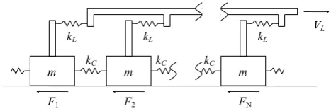
Fig. 1. Illustration of our one-dimensional slider-block model. A linear array ofNblocks of massmare pulled along a surface by a constant velocityVLloader plate. The loader plate is connected to each block with a loader spring with spring constantkLand adja-cent blocks are connected by springs with spring constantkC. The frictional resisting forces areF1, F2,. . . , FN.
3 Slider-block model
In this paper we consider the behavior of a slider-block model in order to study the statistics of the interval times be-tween slip events. We utilize a variation of the linear slider-block model which Carlson and Langer (1989) used to il-lustrate the self-organization of such models. We consider a linear chain of 25, 50, and 100 slider blocks of massmpulled over a surface at a constant velocityVLby a loader plate as
illustrated in Fig. 1. Each block is connected to the loader plate by a spring with spring constantkL. Adjacent blocks
are connected to each other by springs with spring constant kC. Boundary conditions are assumed to be periodic: the last
block is connected to the first one.
The blocks interact with the surface through friction. In this paper we prescribe a static-dynamic friction law. The static stability of each slider-block is given by
kLyi+kC(2yi −yi−1−yi+1) < FSi (5)
whereFSi is the maximum static friction force on blocki
holding it motionless, andyi is the position of blockirelative
to the loader plate.
During strain accumulation due to loader plate motion all blocks are motionless relative to the surface and have the same increase of their coordinates relative to the loader plate
dyi
dt =VL (6)
When the cumulative force of the springs connecting to block iexceeds the maximum static frictionFSi, the block begins
to slide. We include inertia, and the dynamic slip of blocki is controlled by the equation
md 2y
i
dt2 +kLyi+kC(2yi −yi−1−yi+1)=FDi (7) whereFDi is the dynamic (sliding) frictional force on block i. The loader plate velocity is assumed to be much smaller than the slip velocity, requiring
VL FSref √
kLm
100 101 102 10-4
10-3 10-2 10-1 100
Simulation data α = 3 Slope -1.29
NL/NT
L
Fig.2: Abaimov S.G. et al. Recurrence and interoccurence...
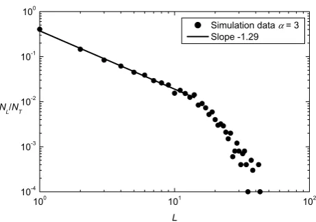
Fig. 2. Frequency-size distribution of 10 000 slip events for a “soft” system withα=3. The ratio of the number of eventsNLof linear sizeLto the total number of eventsNT is given as a function ofL. The solid line is a power-law dependence with exponent –1.29.
0.0 0.1 0.2 0.3 0.4 0.5
0 1
10 -100 block events α = 3 Exponential fit
P(t)
t
Fig.3: Abaimov S.G. et al. Recurrence and interoccurence...
Fig. 3. Cumulative distribution functionP (t )of interoccurrence timestfor the events given in Fig. 2 in the size rangeL=10 to 100. The dashed line is the distribution of observed recurrence times. The continuous line is the best-fit exponential (Poisson) distribu-tion.
so the movement of the loader plate is neglected during a slip event. The sliding of one block can trigger the instability of the other blocks forming a many block event. When the velocity of a block is zero it sticks with zero velocity if the static friction criterion (5) is satisfied, if the criterion is not satisfied the block continues to slip.
It is convenient to introduce the nondimensional variables and parameters
τf=t
r
kL
m, τs= t kLVL
FSref , Yi =kLyi
FSref, φ = FSi
FDi , α=kC
kL , βi=
FSi
FSref (9)
The ratio of static to dynamic frictionφis assumed to be the same for all blocks but the values themselvesβi vary from
block to block withFSref as a reference value of the static
frictional force (FSrefis the minimum value of allFSi). Stress
accumulation occurs during the slow timeτswhen all blocks
are stable, and slip of blocks occurs during the fast timeτf
when the loader plate is assumed to be approximately mo-tionless.
In terms of these nondimensional variables the static sta-bility condition (5) becomes
Yi+α (2Yi −Yi−1−Yi+1) < βi (10)
the strain accumulation Eq. (6) becomes dYi
dτS
=1 (11)
and the dynamic slip Eq. (7) becomes d2Yi
dτf2
+Yi +α (2Yi−Yi−1−Yi+1)= βi
φ (12)
Before obtaining solutions, it is necessary to prescribe the pa-rametersφ,α, andβi. The parameterαis the stiffness of the
system. We first consider the 100 block system and obtain solutions forαfrom 3 to 1000 in this paper. Forα=3 the sys-tem is soft and there are no syssys-tem wide (100 block) events. Forα=1000 the system is stiff and system wide (100 block) events dominate. The ratio φof static friction to dynamic friction is taken to be the same for all blocksφ=1.5, while the values of frictional parametersβi are assigned to blocks
by uniform random distribution from the range 1<βi<3.5.
This random variability in the system is a “noise” required to generate event variability in stiff systems.
The loader plate springs of all blocks extend according to Eq. (11) until a block becomes unstable from Eq. (10). The dynamic slip of that block is calculated using the Runge-Kutta numerical method to obtain a solution of Eq. (12). A coupled 4th-order iterational scheme is used, and all equa-tions are solved simultaneously (the Runge-Kutta coeffi-cients of neighboring blocks participate in the generation of the next order Runge-Kutta coefficient for the given block). The dynamic slip of one block may trigger the slip of other blocks and the slip of all blocks is followed until they all be-come stable. Then the procedure repeats.
240 242 244 246 1.2
1.4 1.6 1.8
Y
τS
Fig.4: Abaimov S.G. et al. Recurrence and interoccurence...
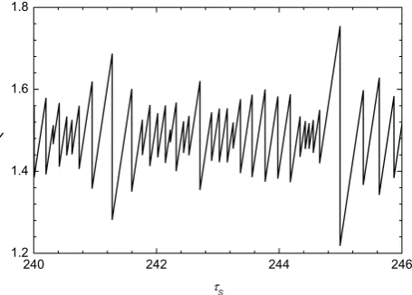
Fig. 4. The nondimensional position of a typical blockY is given as a function of the nondimensional slow timeτS. This is a result for a heterogeneous stiff system withα=1000.
100 101 102
10-4
10-3
10-2
10-1
100
Simulation data α = 1000 Slope -2.12
NL/NT
L
Fig.5: Abaimov S.G. et al. Recurrence and interoccurence...
Fig. 5. Frequency-size distribution of 10 000 slip events for a “stiff” system withα=1000. The ratio of the number of eventsNLof linear sizeLto the total number of eventsNT is given as a function ofL. The solid line is a power-law dependence with exponent –2.12.
and are not correlated. A similar result was obtained for the sandpile model (Sanchez, et al., 2002). Since these smaller events occur at different positions along the array they do not have a memory of previous events.
We next give results for a stiff system withα=1000. With infinite stiffness the system will behave as a rigid body with periodic slip events. The stiff homogeneous system with βi=1 shows a “creeping” behavior in our simulations – it
creeps block by block – only a small number of blocks move simultaneously at any time. The introduction of even a small amount of symmetry-breaking heterogeneity causes system-wide (100 block) events to occur.
For the heterogeneous stiff system with a random distri-bution of friction coefficients 1<βi<3.5 the motion
orga-nizes itself into the recurrence of system-wide (100 block)
0.0 0.1 0.2 0.3 0.4
0 1
100 block events α = 1000 Weibull fit τ = 0.21 γ = 2.60 P(t)
t
Fig.6: Abaimov S.G. et al. Recurrence and interoccurence...
Fig. 6. Cumulative distribution functionP (t )of recurrence times tfor the 1500 system-wide (100 block) events withα=1000. The dashed line is the distribution of observed recurrence times. The continuous line is the best-fit Weibull distribution withτ= 0.21 and γ=2.60.
10-1 100
10-3
10-2
10-1
100
101
100 block events α = 1000 Weibull fit τ = 0.21 γ = 2.60 -ln[1-P(t)]
t/τ
Fig.7: Abaimov S.G. et al. Recurrence and interoccurence...
Fig. 7. Weibull probability plot of the cumulative distribution of recurrence times for the data given in Fig. 6. The solid line corre-sponds to a Weibull distribution as given in Eq. (13) withτ= 0.21 andγ=2.60.
100
10-4
10-3
10-2
10-1
NSW
/
NT
α − αC
Fig.8: Abaimov S.G. et al. Recurrence and interoccurence...
Fig. 8. Dependence of simulation values of the fraction of events that are system-wideNSW/NT on the difference between the stiff-ness of the arrayαand the critical value of this tuning parameter αC. The circles are the results for a 100 block simulation and the solid line is the power-law scaling from Eq. (14) takingαC=4.45 andδ=2.25. The diamonds are the results for a 50 block simulation and the dashed line is the power-law scaling from Eq. (14) taking αC=2.518 andδ=2.47. The triangles are the results for a 25 block simulation and the dashed-dot line is the power-law scaling from Eq. (14) takingαC=0.782 andδ=3.18.
using a “Weibull probability plot”. We rewrite Eq. (1) as − ln(1−P (t ))=
t
τ
γ
(13) In Fig. 7 we plot log [−ln(1−P (t ))] versus logτtfor our data. The Weibull distribution requires a straight-line fit with slopeγ. Takingτ=0.21 andγ=2.60 the fit shown has R2=0.998. The data are well approximated by the straight-line fit.
We have obtained results for other values of the stiffness α. We find that the number of system wide events is virtually independent ofαin the range 50<α<10 000. We also find that the recurrence time statistics satisfy the Weibull distri-bution to a good approximation in this range. The Weibull exponentγslowly decreases fromγ=3.3 atα=100 toγ=2.2 atα=10 000. We have also examined the hypothesis that the onset of system-wide events is a critical point (Grassberger, 2002) and thatαis the relevant tuning parameter. We first consider the ratio of the number of system-wide slip events NSW to the total number of all slip eventsNT. We test the
power-law relation NSW
NT
∝(α−αC)δ (14)
withα>αC.
In order to test the validity of this relation we give re-sults for linear chains of 25, 50, and 100 slider blocks. In Fig. 8 we give the dependenceNSW/NT versus α–αC for
100
100
101
t
α − αC
Fig.9: Abaimov S.G. et al. Recurrence and interoccurence...
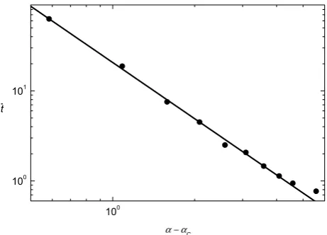
Fig. 9. Dependence of simulation values of the mean non-dimensional time between system-wide eventst¯on the difference between the stiffness of the arrayαand the critical value of this tuning parameterαC=4.42 (solid circles). The straight line is the power-law scaling from Eq. (15) taking the exponentε=2.07.
the three cases. For 25 slider blocks the simulation results are well approximated (R2=0.999) by this scaling relation taking αC=0.782±0.164 and δ=3.18±0.28 (the errors are
95% confidence bounds). For 50 slider blocks the simula-tion results are well approximated (R2=0.998) by Eq. (14) taking αC=2.518±0.182 and δ=2.47±0.28. And for 100
slider blocks the simulation results are again well approx-imated (R2=0.998) by Eq. (14) taking αC=4.45±0.46 and δ=2.25±0.52. The good agreement of our simulation results with the power-law scaling relation (14) is evidence that the onset of system-wide events is a critical point with the stiff-nessαas the tuning parameter. The system-wide events rep-resent a new phase and the critical point is the transition to this phase.
To further test the power-law scaling in the vicinity of a critical point we test two other scaling laws for the 100 slider-block model. We next consider the mean recurrence time between system-wide eventst¯. We test the scaling relation ¯
t ∝(α−αC)−ε (15)
withα>αC. In Fig. 9 we show that our simulations are well
approximated (R2=0.999) by this scaling relation again tak-ingαC=4.42±0.14 and in this caseε=2.07±0.29. We finally
consider the ratio of the energy dissipated in system-wide events to the energy dissipated in all eventse100/eT. We test
the scaling relation e100
eT
∝(α−αC)µ (16)
withα>αC. In Fig. 10 we show that our simulations are
well approximated (R2=0.998) by this scaling relation taking αC=4.57±0.28 and in this caseµ=1.78±0.30. The validity
of system-wide events is a critical point (Goldenfeld, 1992; Stauffer and Aharony, 1992).
The three values of the critical stiffness (αC=4.45±0.46, αC=4.42±0.14, and αC=4.57±0.28) should be equal. The
differences are much smaller than the 95% confidence lim-its. Taking the mean value we obtainαC=4.48±0.17.
An-other question is whether the three exponents (δ=2.25±0.52, ε=2.07±0.29, and µ=1.78±0.30) should be equal. Again the differences are less than the 95% confidence limits. The product of the number of system-wide slip eventsN100 and the mean recurrence time between system-wide events t¯ equals the total time of the simulation – a quantity which does not have a singularity and is a constant in the vicinity of the critical point. This suggests that the exponentsδ and εshould be equal. In the same way the ratio of the energy dissipated in system-wide events during the simulatione100 to the number of system-wide slip eventsN100 is the mean energy dissipated in one system-wide event – also a quan-tity which does not have a singularity and is a constant in the vicinity of the critical point from above. This suggests that the exponentsδ andµshould also be equal. Assuming that the three exponents are equal we findδ=ε=µ=2.03±0.21.
One way to interpret the results we have obtained is in terms of finite-size scaling (Goldenfeld, 1992; Stauffer and Aharony, 1992). Specifically, we consider finite-size scaling within the context of clusters observed in percolation the-ory. Here the system size has lengthL, and the clustering of events is associated with the appearance of a correlation lengthξ. The system boundaries have little or no influence on the problem whenξL. However, when ξ >L, system boundaries introduce cutoffs in cluster size, and are therefore expected to influence the values of percolation thresholds, scaling exponents, and other observed quantities. For exam-ple, the specific valuesαCare affected by the sizeL=25, 50,
and 100 that is used. Whenξ∼L, a variety of crossover ef-fects may be observed.
The behavior of the system depends upon the ratio of the system size to the correlation length. Finite-size effects play a crucial role here, that’s why we investigate the model with only 100 slider-blocks. Changing the stiffness of the system as a tuning parameter is equivalent to changing the ratio of the system size to the correlation length. The critical point is the result of the appearance of system-wide events, and a consequence is the change of the interval statistics from the Poissonian (exponential) below the critical point to the Weibull statistics in the limit of very stiff system.
4 Why Weibull
A primary focus of this paper is on the applicability of the Weibull distribution to the statistics of recurrence times for self-organizing complex phenomena. In the engineering lit-erature this distribution has found wide applicability to the statistics of failure. A standard failure problem is that of
100
10-2
10-1
e100 / eT
α − αC
Fig.10: Abaimov S.G. et al. Recurrence and interoccurence...
Fig. 10. Dependence of simulation values of the fraction of the energy dissipated in system-wide eventse100/eT on the difference between the stiffness of the arrayαand the critical value of this tuning parameterαC=4.57 (solid circles). The straight line is the power-law scaling from Eq. (16) taking the exponentµ=1.78.
fiber bundles which can be associated with composite mate-rials (Newman and Phoenix, 2001). The dynamic failure of a bundle ofN0fibers is modeled empirically by the relation
dN
dt = −N νr
σ
σr p
(17) whereN is the number of remaining fibers andνr is the
ref-erence hazard rate at the refref-erence stressσr. Assuming that
the stress increases linearly in time σ
σr
= t tr
(18) Eq. (17) becomes
dN
dt = −N νr
t
tr p
(19) Integrating withN=N0att=0 gives
N N0
=exp
"
−νrt
p+1
pτp #
(20)
We next introduce P (t )=1− N
N0
, γ =p+1, νr = γ
τ (21)
whereP (t )is the cumulative distribution function of failure. Substituting Eq. (21) into Eq. (20) gives the Weibull distribu-tion Eq. (1). The self-similar (power-law) dependence of the hazard rate on time leads directly to the Weibull distribution of failure times.
just as the forces on our slider blocks increase linearly in time due to the steady motion of the loader plate. Similarly the stress on the fiber bundle as given by Eq. (18) increases linearly with time. We have shown above that the failure rate of a fiber bundle modeled by Eq. (17) gives a Weibull distribution. This provides a basis for the application of the Weibull distribution both to our slider-block model and to characteristic earthquakes.
5 Fractional noises
Another application of the Weibull (stretched exponential) distribution is to fractional noises. Fractional noises and walks are time series with long range power-law correlations. This dependence is generally quantified in terms of a power-law dependence of the power-spectral densitySon frequency f (Malamud and Turcotte, 1999)
S∝f−β (22)
For a stationary fractional noise we have –1≤β≤1. In the range 0<β≤1 adjacent values are correlated, large (small) follows large (small). In the range –1≤β<0 adjacent values are anticorrelated, small (large) follows large (small). Quan-tification of correlations in a fractional noise is done in terms of the autocorrelation functionr(s)(Altmann, et al., 2004; Altmann and Kantz, 2005; Bunde, et al., 2003, 2004; Pen-netta, 2006)
r(s)∝s−γ (23)
wheresis the lag. The exponentsγandβare related by
γ=1−β (24)
For a stationary fractional noise we have 0<γ <2. In the range 0<γ <1 adjacent values are correlated and in the range 1<γ <2 adjacent values are anticorrelated.
Another alternative quantification of the scaling properties of a fractional noise is in terms of rescaled range (R/S) anal-ysis. In this case we have (Malamud and Turcotte, 1999)
R S ∝τ
H u (25)
whereτ is the length of the record and Hu is the Hurst ex-ponent. The three power-law exponents Hu, β, andγ are related by
H u=β+1
2 =
2−γ
2 (26)
For a stationary fractional noise we have 0<Hu<1. In the range 0<Hu<0.5 adjacent values are anticorrelated and in the range 0.5<Hu<1 adjacent values are correlated.
For an uncorrelated white-noise time series we haveβ=0, Hu=0.5, andγ=1. For many natural time series it is found that 0.70≤Hu≤0.80 (Pelletier and Turcotte, 1999). Exam-ples include river discharges, lake levels, varve thicknesses,
sunspot numbers, and atmospheric time series. The corre-sponding values of the exponentsβandγare: 0.40≤β≤0.60 and 0.40≤γ≤0.60.
Recent studies have been carried out on the recurrence statistics of peaks over thresholds for fractional noises (Alt-mann, et al., 2004; Altmann and Kantz, 2005; Bunde, et al., 2003, 2004; Pennetta, 2006). These studies have shown that the recurrence statistics satisfy the Weibull (stretched expo-nential) distribution given in Eq. (1). The exponentγ in the Weibull distribution is equal to exponent for the autocorrela-tion funcautocorrela-tion given in Eq. (23).
For an uncorrelated white noise withγ=1 we have a Pois-son (exponential) distribution from Eq. (1) as expected and the hazard rate from Eq. (4) is constant. For a correlated noise we have 0<γ <1 and the Weibull distribution (1) is a stretched exponential with a hazard function from Eq. (4) that has a power-law decrease with time. For an anticorrelated‘ noise we have 1<γ <2 and the hazard function from Eq. (4) has a power-law increase with time.
6 Conclusions
One purpose of this paper is to demonstrate that the interval statistics of both models and natural systems exhibit Weibull distributions. We argue that the reason for the applicability of the Weibull distribution is that its hazard function as defined in Eq. (4) is a scale-invariant power-law function of time. It is important to make a clear distinction between the pdf of interval times for all events and the hazard function which is the pdf of the interval time for a single event. There is a mean interval for all events and for the Weibull distribution this has been given in Eq. (2). The distribution of all interval times is clearly scale dependent. Instead, consider the behavior of the system after an event has occurred. The pdf of possi-ble interval times until the next event is the hazard function. The Weibull distribution is the only distribution that gives a power-law, scale-invariant distribution of these intervals.
In order to demonstrate the applicability of the Weibull distribution we have considered the behavior of a slider-block model. We have carried out a full dynamic simula-tion using linear arrays of slider blocks. The behavior of the model is governed by its “stiffness”α, the ratio of the con-nector spring constant to the loader spring constant as given in Eq. (9). For low values of α, soft systems, there are no system-wide events. For high values ofα, stiff systems, large number of system-wide events occur in which all blocks slip simultaneously. In order to get system-wide events it was necessary to break the symmetry of the model by introduc-ing a random variability of the friction coefficients.
α=3. In this case the distribution is well approximated by an exponential (Poisson) distribution. An event does not have a significant “memory” of prior events. This is con-sistent with prior studies of SOC models such as the sandpile model (Sanchez, et al., 2002) in which exponential distribu-tions were found.
There have been many papers published on a variety of slider-block models (Turcotte, 1999). In order to reduce computer time almost all utilize a cellular automata approxi-mation, only one block is allowed to slip instead of multiple-block slip events. We have chosen to use a fully dynamic simulation with a relatively small number (100) of blocks. We believe our results are robust both in terms of Weibull statistics and in terms of a well defined critical point.
We argue that there is a direct analogy between the be-havior of our slider-block model and the bebe-havior of actual earthquakes. Characteristic earthquakes are earthquakes that repeatedly occur on a particular fault or fault segment. There is considerable evidence from both actual earthquakes (Hagi-wara, 1974; Rikitake, 1976, 1982, 1991; Utsu, 1984) and simulations (Yakovlev, et al., 2006) that the distribution of recurrence times for a set of characteristic earthquakes on a fault satisfies a Weibull distribution. This is in direct anal-ogy to the behavior of our stiff slider-block model. There is also observational evidence that the interoccurrence times between all earthquakes in a region (on many different faults) satisfy Poissonian statistics (Shcherbakov, et al., 2005). This is in direct analogy to the behavior of our soft slider-block model.
Weibull (stretched exponential) statistics have also been found to be applicable to the distribution of peaks over threshold for fractional Gaussian noises (Altmann, et al., 2004; Altmann and Kantz, 2005; Bunde, et al., 2003; 2004; Pennetta, 2006). Again we argue that this is due to the scale-invariant (power-law) dependence of the hazard function for the Weibull distribution. For correlated fractional noises the probability of the next event decreases as an inverse power of the timet0since the last event as given in Eq. (4). For anti-correlated fractional noises the probability of the next event increases as a power of the time since the last event. This is the behavior associated with characteristic earthquakes and with our “stiff” slider-block simulations.
Acknowledgements. We wish to acknowledge valuable discussions with G. Yakovlev and B. Newman. This work has been supported by NSF Grants ATM 0327571 and ATM 0327799.
Edited by: P. Yiou
Reviewed by: two anonymous referees
References
Altmann, E. G., da Silva, E. C., and Caldas, I. L.: Recurrence time statistics for finite size intervals, Chaos, 14, 975–981, 2004.
Altmann, E. G. and Kantz, H.: Recurrence time analysis, long-term correlations, and extreme events, Phys. Rev. E, 71, 056106, doi:10.1103/PhysRevE.71.056106, 2005.
Bak, P., Christensen, K., Danon, L., and Scanlon, T.: Unified scaling law for earthquakes, Phys. Rev. Lett., 88, 178501, doi: 10.1103/PhysRevLett.88.178501, 2002.
Bak, P., Tang, C., and Wiesenfeld, K.: Self-organized criticality, Phys. Rev. A, 38, 364–374, 1988.
Bakun, W. H., Aagard, B., Dost, B., et al.: Implications for predic-tion and hazard assessment from the 2004 Parkfield earthquake, Nature, 437, 969–974, 2005.
Bunde, A., Eichner, J. F., Havlin, S., and Kantelhardt, J. W.: The ef-fect of long-term correlations on the return periods of rare events, Physica A, 330, 1–7, 2003.
Bunde, A., Eichner, J. F., Havlin, S., and Kantelhardt, J. W.: Return intervals of rare events in records with long-term persistence, Physica A, 342, 308–314, 2004.
Carbone, V., Sorriso-Valvo, L., Harabaglia, P., and Guerra, I.: Uni-fied scaling law for waiting times between seismic events, Euro-phys. Lett., 71, 1036–1042, 2005.
Carlson, J. M. and Langer, J. S.: Mechanical model of an earthquake fault, Phys. Rev. A, 40, 6470–6484, 1989.
Corral, A.: Local distributions and rate fluctuations in a uni-fied scaling law for earthquakes, Phys. Rev. E, 68, 035102(R), doi:10.1103/PhysRevE.68.035102, 2003.
Corral, A.: Long-term clustering, scaling, and universality in the temporal occurrence of earthquakes, Phys. Rev. Lett., 92, 108501, doi:10.1103/PhysRevLett.92.108501, 2004a.
Corral, A.: Universal local versus unified global scaling laws in the statistics of seismicity, Physica A, 340, 590–597, 2004b. Corral, A.: Mixing of rescaled data and Bayesian inference for
earthquake recurrence times, Nonlin. Processes Geophys., 12, 89–100, 2005a.
Corral, A.: Time-decreasing hazard and increasing time until the next earthquake, Phys. Rev. E, 71, 017101, doi:10.1103/PhysRevE.71.017101, 2005b.
Davidsen, J. and Goltz, C.: Are seismic waiting time dis-tributions universal?, Geophys. Res. Lett., 31, L21612, doi:10.1029/2004GL020892, 2004.
Davis, P. M., Jackson, D. D., and Kagan, Y. Y.: The longer it has been since the last earthquake, the longer the expected time till the next, Bull. Seism. Soc. Am., 79, 1439–1456, 1989.
Drossel, B. and Schwabl, F.: Self-organized critical forest-fire model, Phys. Rev. Lett., 69, 1629–1632, 1992.
Gabrielov, A., Newman, W. I., and Turcotte, D. L.: Exactly soluble hierarchical clustering model: Inverse cascades, self-similarity, and scaling, Phys. Rev. E, 60, 5293–5300, 1999.
Goes, S. D. B. and Ward, S. N.: Synthetic seismicity for the San Andreas Fault, Ann. Geofisica, 37, 1495–1513, 1994.
Goldenfeld, N.: Lectures on Phase Transitions and the Renormal-ization Group, Addison Wesley, Reading, MA, 394pp., 1992. Grassberger, P.: Critical behaviour of the Drossel-Schwabl forest
fire model, New J. Phys., 4, 17, doi:10.1088/1367-2630/4/1/317, 2002.
Hagiwara, Y.: Probability of earthquake occurrence as obtained from a Weibull distribution analysis of crustal strain, Tectono-phys., 23, 313–318, 1974.
dis-tributions and scaling laws, Phys. Rev. Lett., 94, 108501, doi:10.1103/PhysRevLett.94108501, 2005.
Livina, V., Havlin, S., and Bunde, A.: Memory in the occurrence of earthquakes, Phys. Rev. Lett., 95, 208501, doi:10.1103/PhysRevLett.95.208501, 2005a.
Livina, V., Tuzov, S., Havlin, S., and Bunde, A.: Recurrence inter-vals between earthquakes strongly depend on history, Physica A, 348, 591–595, 2005b.
Malamud, B. D. and Turcotte, D. L.: Self-affine time series: I. Gen-eration and analyses, Adv. Geophys., 40, 1–90, 1999.
Matthews, M. V., Ellsworth, W. L., and Reasenberg, P. A.: A Brow-nian model for recurrent earthquakes, Bull. Seism. Soc. Am., 92, 2233–2250, 2002.
Newman, W. I. and Phoenix, S. L.: Time-dependent fiber bun-dles with local load sharing, Phys. Rev. E, 63, 021507, doi:10.1103/PhysRevE.63.021507, 2001.
Pelletier, J. D. and Turcotte, D. L.: Self-affine time series: II. Ap-plications and models, Adv. Geophys., 40, 91–166, 1999. Pennetta, C.: Distribution of return intervals of extreme events, Eur.
Phys. J. B, 50, 95–98, 2006.
Rikitake, T.: Recurrence of great earthquakes at subduction zones, Tectonophys., 35, 335–362, 1976.
Rikitake, T.: Earthquake Forecasting and Warning, D. Reidel Pub-lishing Co., Dordrecht, 402pp., 1982.
Rikitake, T.: Assessment of earthquake hazard in the Tokyo area, Japan, Tectonophys., 199, 121–131, 1991.
Rundle, J. B.: A Physical Model for Earthquakes, 2. Application to Southern-California, J. Geophys. Res., 93, 6255–6274, 1988. Rundle, J. B., Rundle, P. B., Donnellan, A., and Fox, G.:
Gutenberg-Richter statistics in topologically realistic system-level earth-quake stress-evolution simulations, Earth Planets Space, 56, 761–771, 2004.
Sanchez, R., Newman, D. E., and Carreras, B. A.: Waiting-time statistics of self-organized-criticality systems, Phys. Rev. Lett., 88, 068302, doi:10.1103/PhysRevLett.88.068302, 2002. Savage, J. C.: Empirical earthquake probabilities from observed
re-currence intervals, Bull. Seism. Soc. Am., 84, 219–221, 1994.
Shcherbakov, R., Yakovlev, G., Turcotte, D. L., and Run-dle, J. B.: Model for the distribution of aftershock interoccurrence times, Phys. Rev. Lett., 95, 218501, doi:10.1103/PhysRevLett.95.218501, 2005.
Sieh, K., Stuiver, M., and Brillinger, D.: A more precise chronology of earthquakes produced by the San-Andreas fault in southern California, J. Geophys. Res., 94, 603–623, 1989.
Sornette, D. and Knopoff, L.: The paradox of the expected time until the next earthquake, Bull. Seism. Soc. Am., 87, 789–798, 1997.
Stauffer, D. and Aharony, A.: Introduction To Percolation Theory, 2nd ed., Taylor & Francis, 181pp., 1992.
Turcotte, D., Malamud, B. D., Morein, G., and Newman, W. I.: An inverse-cascade model for self-organized critical behavior, Phys-ica A, 268, 629–643, 1999.
Turcotte, D. L.: Self-organized criticality, Rep. Prog. Phys., 62, 1377–1429, 1999.
Turcotte, D. L. and Malamud, B. D.: Landslides, forest fires, and earthquakes: examples of self-organized critical behavior, Phys-ica A, 340, 580–589, 2004.
Utsu, T.: Estimation of parameters for recurrence models of earth-quakes, Bull. Earthquake Res. Insti.-Univ. Tokyo, 59, 53–66 1984.
Ward, S. N.: A synthetic seismicity model for southern California: Cycles, probabilities, and hazard, J. Geophys. Res., 101, 22 393– 22 418, 1996, 1996.
Ward, S. N.: San Francisco Bay Area earthquake simulations: A step toward a standard physical earthquake model, Bull. Seism. Soc. Am., 90, 370–386, 2000.
Working Group on California Earthquake Probabilities: Earthquake probabilities in the San Francisco Bay Region, 2002-2031, U.S. Geological Survey, Open-File Report 2003-214, 2003.
Yakovlev, G., Newman, W. I., Turcotte, D. L., and Gabrielov, A.: An inverse cascade model for self-organized complexity and nat-ural hazards, Geophys. J. Int., 163, 433–442, 2005.