www.clim-past.net/6/431/2010/ doi:10.5194/cp-6-431-2010
© Author(s) 2010. CC Attribution 3.0 License.
Climate
of the Past
Interhemispheric coupling, the West Antarctic Ice Sheet and warm
Antarctic interglacials
P. B. Holden1, N. R. Edwards1, E. W. Wolff2, N. J. Lang2, J. S. Singarayer3, P. J. Valdes3, and T. F. Stocker4
1Earth and Environmental Sciences, Open University, Milton Keynes, UK 2British Antarctic Survey, Cambridge, UK
3School of Geographical Sciences, University of Bristol, Bristol, UK 4Climate and Environmental Physics, University of Bern, Bern, Switzerland
Received: 27 November 2009 – Published in Clim. Past Discuss.: 17 December 2009 Revised: 6 July 2010 – Accepted: 7 July 2010 – Published: 16 July 2010
Abstract. Ice core evidence indicates that even though at-mospheric CO2concentrations did not exceed∼300 ppm at
any point during the last 800 000 years, East Antarctica was at least∼3–4◦C warmer than preindustrial (CO2∼280 ppm)
in each of the last four interglacials. During the previous three interglacials, this anomalous warming was short lived (∼3000 years) and apparently occurred before the comple-tion of Northern Hemisphere deglaciacomple-tion. Hereafter, we refer to these periods as “Warmer than Present Transients” (WPTs). We present a series of experiments to investigate the impact of deglacial meltwater on the Atlantic Meridional Overturning Circulation (AMOC) and Antarctic temperature. It is well known that a slowed AMOC would increase south-ern sea surface temperature (SST) through the bipolar seesaw and observational data suggests that the AMOC remained weak throughout the terminations preceding WPTs, strength-ening rapidly at a time which coincides closely with peak Antarctic temperature. We present two 800 kyr transient sim-ulations using the Intermediate Complexity model GENIE-1 which demonstrate that meltwater forcing generates transient southern warming that is consistent with the timing of WPTs, but is not sufficient (in this single parameterisation) to repro-duce the magnitude of observed warmth. In order to inves-tigate model and boundary condition uncertainty, we present three ensembles of transient GENIE-1 simulations across Termination II (135 000 to 124 000 BP) and three snapshot HadCM3 simulations at 130 000 BP. Only with consideration of the possible feedback of West Antarctic Ice Sheet (WAIS) retreat does it become possible to simulate the magnitude of observed warming.
Correspondence to: P. B. Holden
(p.b.holden@open.ac.uk)
1 Introduction
The AMOC transports a substantial amount of heat from south to north. If the AMOC is weakened through changes in surface buoyancy, Northern Atlantic cooling and South-ern Atlantic warming is simulated in ocean models of var-ious complexities (Stouffer et al., 2006). This effect, the bipolar seesaw, has been proposed (Stocker and Johnsen, 2003) to explain the interhemispheric teleconnection of abrupt millennial-scale shifts in glacial climate known as Dansgaard-Oeschger (DO) events (Dansgaard et al., 1993). We here address the proposed role of the bipolar seesaw in defining the characteristics of glacial terminations and the in-terglacials which follow them (Ganopolski and Roche, 2009; Masson-Delmotte et al., 2010).
30 Figure 1
a
b
c
kyr BP
a
b
c
kyr BP
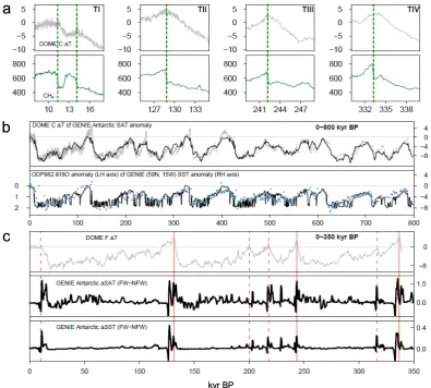
Fig. 1. (a) DOME CδD-inferred Antarctic temperature anomaly (Jouzel et al., 2007) (grey) and atmospheric CH4concentration (Loulergue et al., 2008) (green) at the last four terminations. (b) 800 kyr records of DOME C Antarctic temperature anomaly (grey) and planktonicδ18O anomaly (blue) at ODP site 982 (57.3◦N, 15.5◦W) (Venz et al., 1999), compared respectively with the GENIE-1 (GFW)Antarctic SAT anomaly and the SST anomaly at the grid cell centred on 59◦N, 15◦W. (c) 350 kyr records of DOME FδD-inferred Antarctic temperature anomaly (Kawamura et al., 2007) (grey), GENIE-1 meltwater-induced (GFW-GNFW)Antarctic SAT and SST anomalies. SAT is averaged over Antarctica south of 71◦S. SST is averaged over all the Southern Ocean south of 62◦S. Note: the simulation in (b) includes meltwater forcing, but the effects in Antarctica (up to∼1.5◦C warming) are largely obscured by the larger changes across the terminations.
In contrast, the three previous terminations (TII, TIII and TIV) exhibit a behaviour that is quite distinct from TI, al-though they display remarkable similarities to one another. In each case a transient spike in Antarctic temperature (WPT) of up to∼4◦C lasting∼3 kyr is apparent at the start of the interglacial. Recent analysis (Sime et al., 2009) suggests that the isotopic composition of East Antarctic ice is less sensi-tive to temperature change in a warm climate, consistent with even higher peak Antarctic temperatures during these inter-glacials (at least∼6◦C warmer than present day), though this work did not consider the warming mechanism of the bipolar seesaw that is addressed here. Observational evi-dence for WPTs in Antarctica is not confined to ice-core records. Notably, a 430 kyr Southern Ocean SST reconstruc-tion (Cortese et al., 2007) at ODP site 1089 (41◦S 10◦E)
displayed transient warming during each of these termina-tions, lasting for 5–9 kyrs and with temperatures 2 to 3.5◦C warmer than present (in addition to a∼2◦C transient warm-ing lastwarm-ing for 7 kyr durwarm-ing TI). GCM simulations have thus far failed to produce a warmer Antarctica during the last in-terglacial (e.g. Montoya et al., 2000; Groll et al., 2005; Otto-Bliesner et al., 2006; Masson-Delmotte et al., 2010).
speleothem δ18O (Wang et al., 2001; Cheng et al., 2006, 2009), a proxy for Asian Monsoon strength, which further suggests a role of the bipolar seesaw during terminations (Cheng et al., 2009). The “Weak Monsoon Intervals” (Cheng et al., 2009) which precede each of the methane shifts ap-proximately coincide with peaks in ice rafted debris in the North Atlantic ODP 980 core (McManus et al., 1999), sup-porting the view that these changes were associated with dis-integrating Northern Hemisphere ice sheets.
Recent climate model simulations have addressed this po-tential mechanism for early interglacial warmth. A simu-lation with the IPSL GCM which included a parameterisa-tion of Greenland melt at 126 kyr BP predicted year-round warming of 0.5◦C in Antarctica, thus implicating the bipo-lar seesaw as a possible driver of transient warmth in MIS 5.5 (Masson-Delmotte et al., 2010). Ganopolski and Roche (2009) performed idealised transient experiments across a glacial termination with CLIMBER-2, an Intermediate Com-plexity model which includes a 2.5-D statistical-dynamical atmosphere model coupled to a zonally-averaged, three-basin ocean model. These simulations produced∼2◦C tran-sient Antarctic warming in response to 0.2 Sv freshwater flux into the North Atlantic and suggested that the qualitative dif-ferences between recent terminations may result from mod-est differences in the rate of deglaciation.
It has recently been suggested that the suppression of DO events (which would cool Antarctica) enables terminations to progress unchecked (Wolff et al., 2009). Here we pro-pose, following Ganopolski and Roche (2009), that if the AMOC remains weakened throughout the termination the system will progress to a WPT state. Furthermore, we pro-pose the WPT may eventually lead to partial collapse of the WAIS, leading to further warming. Thus although the ra-diative forcing due to Northern Hemisphere ice sheets and greenhouse gases was similar to preindustrial in the each of the last three interglacials, weakened overturning together with potential WAIS retreat lead to conditions in Antarctica during the early stages of these interglacials which were sig-nificantly warmer than modern. The resumption of overturn-ing, associated with the cessation of deglaciation meltwater, subsequently cools Antarctica to conditions that are compa-rable to present day.
In order to examine the temporal history of Northern Hemisphere meltwater feedbacks on Antarctic climate, and evaluate the modelling and boundary condition uncertainty, we have performed three sets of experiments. The approach, building on Holden et al. (2010), is designed to allow for the uncertainty that arises from structural error, the irreducible error that remains when the “best” parameters are applied to a model (Rougier, 2007). The multi-millennial transient sim-ulations required here can only be performed with an inter-mediate complexity model. We use GENIE-1 (Lenton et al., 2006), built around a low resolution 3D frictional geostrophic ocean model. An ensemble approach is essential to quantify modelling uncertainty that arises from structural limitations
of such a model. Furthermore, we supplement the GENIE-1 ensembles with simulations using the Hadley centre coupled model HadCM3 (Gordon et al., 2000) in order to investigate robustness with respect to specific structural limitations, es-pecially related to the lack of a dynamic atmosphere. The three experiments are:
i) Two transient 800 kyr simulations with GENIE-1, one which includes the effects of glacial meltwater on ocean circulation and one which neglects this feedback. These simulations provide a long time-series comparison be-tween observations and model results and allow a qual-itative assessment of the role of meltwater in determin-ing transient Northern Atlantic and Antarctic tempera-tures.
ii) Three ensembles of GENIE-1 transient simulations over glacial termination TII, applying the LGM Plausibil-ity Constrained (LPC) parameter set which covers the range of large-scale feedback strength displayed by multi-model GCM ensembles (Holden et al., 2010). These ensembles enable quantification of both mod-elling and boundary condition uncertainties, including an evaluation of potential WAIS retreat feedbacks. iii) Three equilibrium simulations with HadCM3 at
130 000 BP, performed to investigate the robustness of the conclusions derived from GENIE-1, in particular with respect to its simplified atmosphere and snow models.
2 Methods 2.1 GENIE-1
31
Figure 2
-180 -90 0 90 180
-90 -45 0 45 90
Longitude [E]
La
tit
ud
e
[
N
]
-40 -30 -20 -10 0 10 20 30 40
-180 -90 0 90 180
-90 -45 0 45 90
Longitude [E]
La
tit
ud
e
[
N
]
0 1 2 3 4 5 6 7 8 9 10
-20 0 20 40 60 80
-5 -4 -3 -2 -1 0
-5 0 5 10 15 20
-20 0 20 40 60 80
-5 -4 -3 -2 -1 0
0 1 2 3 4 5 6
a: LPC average preindustrial SAT
(ºC) ºC
Sv Sv
b: Standard deviation LPC preindustrial SAT
c: LPC average preindustrial Atlantic overturning d: Standard deviation LPC preindustrial Atlantic overturning
-180 -90 0 90 180
-90 -45 0 45 90
Longitude [E]
La
tit
ud
e
[
N
]
-40 -30 -20 -10 0 10 20 30 40
-180 -90 0 90 180
-90 -45 0 45 90
Longitude [E]
La
tit
ud
e
[
N
]
0 1 2 3 4 5 6 7 8 9 10
-20 0 20 40 60 80
-5 -4 -3 -2 -1 0
-5 0 5 10 15 20
-20 0 20 40 60 80
-5 -4 -3 -2 -1 0
0 1 2 3 4 5 6
a: LPC average preindustrial SAT
(ºC) ºC
Sv Sv
b: Standard deviation LPC preindustrial SAT
c: LPC average preindustrial Atlantic overturning d: Standard deviation LPC preindustrial Atlantic overturning
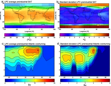
Fig. 2. Ensemble average and standard deviation of preindustrial (a, b) SAT (◦C) and (c, d) Atlantic overturning stream function (Sv). Data are derived from the LPC (LGM Plausibility Constrained) parameter set (Holden et al., 2010).
The 800 kyr simulations (experimental set-up described in Sect. 2.1.1) are performed with the traceable parameter set (Lenton et al., 2006). The TII ensembles (Sect. 2.1.2) are performed using the LPC parameter set (Holden et al., 2010). The LPC averaged preindustrial surface air tempera-ture (SAT) and Atlantic overturning stream function are re-produced in Fig. 2, together with ensemble standard devi-ations. The LPC ensemble exhibits a cold Antarctic bias, with Antarctic SAT−31±10◦C (∼10◦C cooler than NCEP data), likely a result of enforcing modern plausible sea-ice coverage; GENIE is known to underestimate Antarctic sea-ice (Lenton et al., 2006). The major shortcoming of ocean circulation in this configuration of GENIE is the failure of AABW to penetrate into the Atlantic sector (Lunt et al., 2006). However, the LPC parameter set has been designed to exhibit a wide range large-scale feedback strengths (see Sect. 2.1.2) that generally encompass the range of GCM re-sponses to both LGM and 2×CO2 forcing (Holden et al.,
2010).
In both GENIE-1 experiments, changing atmospheric CO2
is prescribed from ice core records (Luethi et al., 2008). Other greenhouse gases are neglected. We apply the orbital forcing of Berger (1978). Transient Laurentide and Eurasian Ice Sheets are represented by interpolating the spatial distri-bution of Ice-4G (Peltier, 1994) onto the benthicδ18O record
(Lisiecki and Raymo, 2005). We derive three variables for each grid cell representing (a) the threshold valueδ18Oth at
which the grid cell becomes ice covered, (b) the present-day orography h0 and (c) the incremental orography h1 at
maximum attainable ice thickness. Whenδ18O> δ18Oth, the
height of the ice surface h at each cell is given by the saturat-ing relationship
h=h0+h1
(δ18O−δ18Oth)
(δ18O−δ18O th+k)
(1) whereh1 is derived at each cell to give the Ice-4G height
h=hLGM when δ18O =δ18OLGM. The threshold for ice
coverδ18Othis derived from Ice-4G reconstructions at 1 kyr
or Eurasian Ice-4G ice remains). When δ18O> δ18OLGM,
ice sheets are allowed to thicken (but not expand laterally) beyond the Ice-4G LGM configuration. This assumption leads to minimum sea-levels at 433 kyr BP that are 6 m lower than at the LGM. We note that the only effects of sea-level change represented in GENIE-1 are on ocean salinity (and other ocean tracers when applicable).
Changing ice volume is translated into meltwater fluxes at each grid cell, routed to the Atlantic, Pacific and Arctic Oceans assuming modern topography. Accumulating ice is represented by reduced run-off. This ensures that freshwater fluxes are spatially and temporally consistent with the repre-sentation of the ice sheets, and avoids the problems associ-ated with an unrealistic treatment of salt compensation which is responsible for much of the uncertainty in the far-field re-sponse to freshwater forcing (Stocker et al., 2007). Only the Laurentide and Eurasian Ice Sheets, which account for ∼80% of global ice-sheet change (Peltier, 2004), are allowed to change. This eliminates the potentially confounding ef-fects of assuming synchronous Antarctic meltwater on ocean circulation; it is well known that millennial-scale Southern and Northern Hemisphere changes are likely to be out of phase (Blunier et al., 1998). A scaling of the freshwater flux (parameter “FFX”, default value 1.5) is applied to correct for isostatic depression at the ice-bedrock interface (which we do not model) and for the assumption of a fixed land-sea mask; each of these simplifications would otherwise produce a∼20% underestimation of ice-sheet volume.
The simulations apply an Atlantic-Pacific freshwater flux adjustment (parameter “APM”) to correct for the∼0.29 Sv underestimation of atmospheric moisture transport, required to maintain a stable Atlantic overturning (Edwards and Marsh, 2005). The flux adjustment is held constant during each transient simulation. GCM simulations suggest an un-certainty of ±0.15 Sv in this flux, especially relevant to cli-mate states that differ from modern (Zaucker and Broecker, 1992). However, although the neglect of atmospheric trans-port feedbacks quantitatively alters the modelled sensitivity to transient meltwater fluxes (Marsh et al., 2004), the ensem-ble is designed to cover the range of possiensem-ble sensitivities, varying APM in the range 0.05 to 0.64 Sv across the LPC ensemble members.
2.1.1 Transient GENIE-1 800 kyr simulations
The climatology of the traceable parameter set used in the 800 kyr simulations is discussed in detail elsewhere (Lenton et al., 2006). The equilibrium climate sensitivity of this pa-rameterisation to a doubling of CO2is 3.4◦C, slightly higher
than the value of 3.2◦C in the configuration of Lenton et al. (2006) due to the increased snow albedo feedback that arises from the inclusion of a lapse rate-related orography effect for temperature-driven surface processes. A lapse rate adjustment is not applied for atmospheric processes as these represent averages through the depth of the 1-layer
atmo-sphere. Surface air temperature is thus calculated (and pre-sented throughout) in terms of a sea-level equivalent. Two simulations are performed: GFW, which includes the effects
of glacial meltwater on ocean circulation (FFX = 1.5), and GNFWwhich neglects this feedback (FFX = 0).
2.1.2 Transient GENIE-1 Termination II ensembles Three ensembles of transient simulations over TII (provid-ing approximate analogues for TIII and TIV) are performed, differing in the boundary conditions applied in order to in-vestigate uncertainties in forcing. Ensemble members are weakly constrained to produce plausible preindustrial and LGM climate states by applying the 480 member LPC pa-rameter set, which varies 26 papa-rameters over wide ranges (see Table 1 of Holden et al., 2010). The LPC parameters produce modern-plausible global average SAT, Atlantic over-turning, Antarctic sea-ice coverage and land carbon storage, with distributions that are approximately centred on observa-tions, and are additionally constrained to simulate plausible LGM Antarctic cooling (of 6–12◦C), though we note that glacial cooling of Antarctica may be overstated due to diffu-sive heat transport that is driven by cooling due to Northern Hemisphere ice sheets. The approach is designed to quantify model error by allowing parametric uncertainty to dominate over structural error. The ensemble members exhibit a wide range of ocean, atmospheric, sea-ice and vegetation feedback strengths which generally encompass the range of large-scale GCM responses to 2×CO2and LGM forcing, with a
distri-bution for climate sensitivity of 3.8±0.6◦C and for LGM
globally averaged cooling of 5.9±1.2◦C (c.f. 5.8±1.4◦C, Schneider von Deimling et al., 2006).
The three ensembles are:
i) EFWwhich includes the impact of meltwater runoff on
ocean circulation (Sect. 2.1) and allows for uncertainty in the strength of this feedback by varying FFX (in ad-dition to 25 other parameters), uniformly distributed in the range 1 to 2,
ii) ENFWwhich neglects the role of meltwater (FFX = 0 in
all ensemble members), and
iii) EWAISwhich is identical to EFW except that the WAIS
is replaced with land at sea level. Ice-sheet mod-els (Pollard and DeConto, 2009) have simulated sub-stantial WAIS retreat driven by sea-level rise at termi-nations (neglecting the additional bipolar forcing ad-dressed here). Several lines of indirect evidence sug-gest that WAIS retreat contributed to the observed el-evated sea levels during the last interglacial (Overpeck et al., 2006; Kopp et al., 2009). We capture the un-certainty associated with the degree and timing of po-tential WAIS retreat through the two extreme boundary conditions of EFWand EWAIS. The modern WAIS
we assume the WAIS is removed and replaced entirely by ice-free land in the EWAISensemble. We note that
replacing WAIS with ocean instead of land was found to simulate slightly higher peak Antarctic SAT anoma-lies (2.8◦C c.f. 2.2◦C) in exploratory 650 kyr transient GENIE-1 simulations not described here.
Melting of the WAIS, triggered by sea-level rise or local warming, would release meltwater to the southern ocean, potentially reducing convection and hence reducing local warming (Weaver et al., 2003; Swingedouw et al., 2009). Given the substantial uncertainties involved, however, we do not attempt to model this feedback in the present study. A hosing flux of 0.1 Sv into the Southern Ocean applied for 1000 years (equivalent in magnitude to the complete loss of WAIS ice in 650 years) simulated Antarctic SAT cooling of ∼0.5◦C in the preindustrial climate state (Swingedouw et al., 2009). Transient Southern Ocean cooling events of this mag-nitude would not be inconsistent with “cooling rebounds” of up to∼1◦C that have been observed in several high
south-ern latitude locations during the later stages of each of the last five terminations (Cortese et al., 2007, and references therein).
Transient CO2, orbit and ice sheets are applied as for the
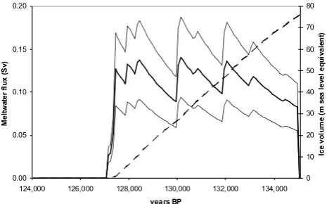
long simulations, except that the benthicδ18O record is lin-earised across the termination to produce an approximately constant (±20%) meltwater pulse, eliminating the oscilla-tory behaviour simulated during TII in the 800 kyr simulation (see Fig. 1c). This oscillatory behaviour is not apparent in observations and is largely a consequence of translating the temporal signal in the gradient of benthicδ18O into global ice-sheet change. The temporal development of ice sheet volume (only Laurentide and Eurasian ice sheets contribu-tions are considered here) and the resulting meltwater flux is illustrated in Fig. 3. As in the 800 kyr simulation, melt-water is routed into the ocean assuming modern topography. The meltwater pulse commences at 135 000 BP and lasts for ∼7600 years with an average of∼0.11 Sv, equivalent to 76 m sea level, but varying between ensemble members (∼0.07 to 0.15 Sv) through the freshwater scaling parameter FFX. Sim-ulations are spun-up to equilibrium at 135 000 BP and run for 11 000 years.
2.2 HadCM3 snapshot simulations
The snapshot simulations are performed using the Hadley Centre coupled model HadCM3 (Gordon et al., 2000), a coupled atmosphere (2.5◦×3.75◦×19 vertical levels)/ocean
(1.25◦×1.25◦×20 vertical levels) model which does not
require flux adjustments to prevent climate drifts. Bound-ary conditions are (HPI)preindustrial, (HNFW)130 000 BP
orbit and greenhouse gases (CO2 256 ppm, CH4 506 ppb,
N2O 239 ppb) with modern ice sheets and no meltwater
flux, (HFW)as HNFWwith 1 Sv North Atlantic hosing (large
enough to ensure collapse on timescales which can be prac-tically simulated) and (HWAIS)as HFWwith WAIS replaced
32 Figure 3
0.00 0.05 0.10 0.15 0.20
124,000 126,000 128,000 130,000 132,000 134,000 years BP
M
e
lt
w
at
e
r
fl
u
x
(
S
v)
0 10 20 30 40 50 60 70 80
Ic
e
v
o
lu
m
e
(m
s
ea
l
e
ve
l
e
q
u
iv
a
le
n
t)
Fig. 3. Representation of ice sheets in the TII ensembles. The
global distribution of ice sheets is given by Equation 1, assuming a constant reduction ofδ18O from 4.86 to 3.16‰ from 135 000 to 126 000 BP. Meltwater is calculated at each grid cell and routed to the ocean assuming modern day topography. The dashed line illus-trates total Laurentide and Eurasian ice sheet volume, expressed in equivalent meters of sea-level. The solid lines illustrates the profile of ensemble mean meltwater flux (bold, FFX = 1.5) and the range of meltwater fluxes (FFX = 1.0 to FFX = 2.0). The temporal devel-opment of meltwater is fixed across all ensemble members.
entirely by ice-free land (at an elevation of 200 m), in or-der to avoid ocean time-stepping instabilities which arise due to converging meridians near the pole (which are resolved with Fourier filtering at the North Pole). As noted above, in GENIE-1 simulations, replacing WAIS with ocean rather than land resulted in a modest increase in warming. Simula-tions are run for 200 years (from the modern spun-up state) and averaged over the last 30 years.
3 Results
3.1 800 kyr GENIE-1 Transient Simulations
Figure 1b compares 800 kyr records of i) modelled Antarc-tic SAT anomaly with DOME C (Jouzel et al., 2007) and ii) modelled SST anomaly (with a North Atlantic planktonic δ18O record (Venz et al., 1999) which we have mapped onto the LR04 timescale (Lisiecki and Raymo, 2005). Model data are from the simulation GFW(which includes meltwater
orbitally-forced summer warming is simulated at high northern lat-itudes during the Eemian, with maximum summer warm-ing (averaged over all grid points north of 62◦N) peaking
at 3.5◦C in 126 000 BP.
The first plot in Fig. 1c is the 350 kyr DOME F tem-perature record, reconstructed from δ18O and δD isotopic records, correcting for vapour source temperature and seawa-ter isotopic composition variations (Kawamura et al., 2007). DOME F was chosen as it lies south of the Atlantic (77◦S, 39◦E) and may be expected to be more strongly influenced by AMOC changes than DOME C (75◦S, 123◦E). In addi-tion to the WPTs, and the warm spike in the early Holocene, three interstadials at DOME F are warmer than preindus-trial at 317, 218 and 200 kyr BP. These three interstadials are observed to be at least∼1◦C cooler than preindustrial at DOME C (Fig. 1b), though we note that these apparent tem-perature differences between DOME C and DOME F may al-ternatively reflect spatial variations in the seasonality of pre-cipitation in a warm Antarctica (Sime et al., 2009).
Antarctic SAT and SST meltwater anomalies (GFW-GNFW,
i.e. the differences in temperature when meltwater is im-posed) are plotted in Fig. 1c and reflect the impact of water on ocean circulation and heat transport. The SAT melt-water anomaly displays the millennial variability apparent in observations; the SST meltwater anomaly exhibits a simi-lar temporal behaviour, though variability is suppressed by high-latitude sea ice during glacial periods. The SST melt-water spikes coincide very closely with spikes in isotope-inferred temperature. Late Pleistocene LR04 age-model un-certainty (the age model which defines the meltwater timing through the gradient of the benthicδ18O) is estimated at 4 kyr (Lisiecki and Raymo, 2005).
The timing of large scale meltwater spikes reflects large changes inδ18O and is likely to be robust (though subject to the aforementioned age-model uncertainties). However, this is not the case with respect to the detail and timing of the millennial variability, including that which is simulated during terminations. These features arise from variability in the gradient of the benthicδ18O signal, which translates into the meltwater fluxes. Although variability in ice-sheet melt rates presumably contributes to this signal, contributions also arise from a number of additional sources, notably includ-ing uncertainty in observational values ofδ18O; 1σ errors of up to∼0.1‰ (Lisiecki and Raymo, 2005) are compara-ble to the average millennial decrease of ∼0.2‰ across a termination. The transient Antarctic SAT cooling of∼1◦C
that occurs at the end of each termination (Fig. 1c) arises due to the positive Atlantic overturning cell extending further south during the reorganisation of the circulation at the end of the meltwater pulse. We note that in the ensemble analysis (Sect. 3.2) this transient cooling generally arises in those sim-ulations in which the AMOC recovers. Amongst these 155 simulations, ensemble averaged cooling of 0.9±0.9◦C oc-curs 1400±900 years after the cessation of meltwater. This may not be a robust feature of the simulations, especially
given the abrupt cessation of the forcing (Fig. 3). The cool-ing does not arise in the TII ensemble average (c.f. blue and pink curves in Fig. 4e), in part due to differences in the tim-ing of these cooltim-ing events and in part due to the masktim-ing effect of the 19 simulations in which the AMOC does not recover and Antarctica remains warm.
3.2 GENIE-1 ensembles of transient simulations over Termination II
Although there is strong chronological similarity between observed and simulated warming, the magnitude of Antarctic SAT spikes in the single 800 kyr simulation GFW(∼1.5◦C,
Fig. 1c and seen in Fig. 1b as small oscillations near the top of each simulated SAT rise) is insufficient to explain the ob-served warmings of ∼4◦C above present (Fig. 1b).
Quan-tification of the discrepancy requires an assessment of mod-elling uncertainities; we apply an ensemble methodology to ascertain the most probable model response and quantify un-certainty.
The 480 meltwater-forced ensemble members EFW
univer-sally exhibited weakened overturning during the termination (average weakening at 128 000 BP of 9±5 Sv with respect to preindustrial). Antarctic SAT at 128 000 BP is >0.5◦C warmer than preindustrial in 110 of these simulations, all of which exhibited a collapse of overturning (peak overturning <6 Sv north of 44◦N), demonstrating that AMOC collapse is required for significant Antarctic warming in GENIE-1. We confine analysis to the 174 parameter sets with maximum overturning<6 Sv to quantify the range of response.
Figure 4a illustrates the meltwater-forced SST anomaly at 128 500 BP (EFW-ENFW, i.e. the ensemble-averaged change
in SST when meltwater is imposed) and displays the char-acteristic behaviour of the bipolar seesaw, although cer-tain atmospheric feedbacks, such as the southward shift of the ITCZ, cannot be captured by the fixed-wind field EMBM. South of 62◦S, ensemble-averaged SST warming of 0.4±0.3◦C is simulated (uncertainties are expressed as 1σ ensemble standard deviations throughout). Modern obser-vations indicate that basal melt rates at the WAIS grounding line increase by∼1 m yr−1for a 0.1◦C increase in SST (Rig-not and Jacobs, 2002), suggesting that the simulated warm-ing may be significant for WAIS instability. Ice-sheet mod-elling has indicated that a 10 myr−1 increase in Antarctic basal melt rates leads to sea level rise of∼25 cm per cen-tury (Huybrechts and de Wolde, 1999). The ensemble de-sign allows a wide range of sea-ice responses, with annual average Antarctic sea ice extent increasing by 9–15 million km2under LGM forcing and decreasing by 5–9 million km2 under 2×CO2 forcing (Holden et al., 2010).
(Nuern-33 Figure 4 -6 -4 -2 0 2 4 6
124,000 126,000 128,000 130,000 132,000 134,000
years BP E a s t A n ta rc ti c S A T A n o m a ly ( ºC ) 0 2 4 6 8 10 12 14 16 18 20 A tl a n ti c O v e rt u rn in g ( S v ) 0 10 20 30 40 50 60
-4 -3 -2 -1 0 1 2 3 4 5 6
Antarctic SAT anomaly relative to modern (C)
N u m b e r o f en se m b le m em b e rs
-180 -90 0 90 180
-90 -45 0 45 90 Longitude [E] La tit ud e [ N ]
-10 -5 0 5
-180 -90 0 90 180
-90 -45 0 45 90 Longitude [E] La tit ud e [ N ]
-10 -5 0 5
-180 -90 0 90 180
-90 -45 0 45 90 Longitude [E] La tit ud e [ N ]
-10 -5 0 5
-180 -90 0 90 180
-90 -45 0 45 90 Longitude [E] La tit ud e [ N ]
-4 -3 -2 -1 0 1 2
a
c
d
b
f
e
Meltwater induced SST anomaly SAT anomaly to modern (no meltwater)
SAT anomaly to modern (meltwater included) SAT Anomaly to modern (meltwater included & no WAIS)
ºC ºC ºC ºC -6 -4 -2 0 2 4 6
124,000 126,000 128,000 130,000 132,000 134,000
years BP E a s t A n ta rc ti c S A T A n o m a ly ( ºC ) 0 2 4 6 8 10 12 14 16 18 20 A tl a n ti c O v e rt u rn in g ( S v ) 0 10 20 30 40 50 60
-4 -3 -2 -1 0 1 2 3 4 5 6
Antarctic SAT anomaly relative to modern (C)
N u m b e r o f en se m b le m em b e rs
-180 -90 0 90 180
-90 -45 0 45 90 Longitude [E] La tit ud e [ N ]
-10 -5 0 5
-180 -90 0 90 180
-90 -45 0 45 90 Longitude [E] La tit ud e [ N ]
-10 -5 0 5
-180 -90 0 90 180
-90 -45 0 45 90 Longitude [E] La tit ud e [ N ]
-10 -5 0 5
-180 -90 0 90 180
-90 -45 0 45 90 Longitude [E] La tit ud e [ N ]
-4 -3 -2 -1 0 1 2
a
c
d
b
f
e
Meltwater induced SST anomaly SAT anomaly to modern (no meltwater)
SAT anomaly to modern (meltwater included) SAT Anomaly to modern (meltwater included & no WAIS)
ºC ºC
ºC ºC
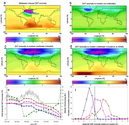
Fig. 4. GENIE-1 ensemble-averaged SST and SAT anomalies. Fields (at 128 500 BP) of (a) meltwater induced SST anomaly (EFW -ENFW)and (b, c, d) SAT anomalies relative to an equilibrium preindustrial ensemble EPI with (b) no meltwater flux (ENFW-EPI), (c) including Laurentide and Eurasian meltwater fluxes (EFW-EPI)and (d) including Laurentide and Eurasian meltwater fluxes and replacing West Antarctic Ice Sheet with land at sea-level (EWAIS-EPI). (e) Ensemble-averaged temporal behaviour of East Antarctic SAT anomaly. The dashed green line is the ensemble-averaged (EFW)Atlantic overturning (maximum streamfunction at depths below 400 m). The grey line is the DOME C deuterium inferred anomaly (Jouzel et al., 2007). Solid lines are East Antarctic SAT anomalies with blue: no meltwater forcing (ENFW-EPI), pink: meltwater forcing included (EFW-EPI), brown: meltwater forcing included and WAIS removed to land at sea level (EWAIS-EPI). (f) Ensemble distributions of East Antarctic SAT anomaly at 128 500 BP.
berg et al., 1997). The ensemble member with the largest meltwater-induced loss of annually-averaged Antarctic sea ice (7.9 million km2)is associated with an East Antarctic SAT 2.4◦C warmer than preindustrial, while the greatest East Antarctic warming, 4.7◦C above preindustrial, is associated with the loss of 4.8 million km2 of Antarctic sea-ice. Thus the possibility that WPTs could be explained without a sub-stantial WAIS retreat feedback appears unlikely (only six of the 174 EFWsimulations exhibit East Antarctic temperatures
greater than 2.5◦C above preindustrial), but cannot be ruled
out.
Figure 4b–d illustrates ensemble-averaged SAT anomalies at 128 500 BP with respect to an equilibrium ensemble EPI
forced with preindustrial boundary conditions. In the ab-sence of meltwater forcing (Fig. 4b), East Antarctic SAT is 1.0±0.6◦C cooler than preindustrial (despite slightly higher atmospheric CO2 concentrations of ∼285 ppm). This
pre-dicts annually averaged Antarctic temperatures 0.6◦C below
preindustrial at this time (ice sheets and atmospheric CO2
fixed at glacial conditions throughout). Meltwater forcing (Fig. 4c) increases East Antarctic SAT by 1.6±1.0◦C (to 0.5±1.0◦C warmer than preindustrial). In these simula-tions, the bipolar warming of Antarctica peaks in the At-lantic sector (i.e. in the vicinity of the forcing), with maxi-mum warming at∼15◦E (Fig. 4c), in the approximate vicin-ity of DOME F. This is qualitatively consistent with observa-tions which indicate that interstadial temperatures may have been higher at DOME F than at DOME C. The removal of WAIS (Fig. 4d) introduces further East Antarctic warming of 1.2±0.6◦C (to 1.6±1.3◦C warmer than preindustrial) aris-ing from widespread loss of West Antarctic summer snow cover and reduced albedo. Within ensemble EWAIS, 39 of the
174 simulations exhibit East Antarctic temperatures greater than 2.5◦C above preindustrial.
Figure 4e summarises the temporal development of ensemble-averaged East Antarctic SAT under the three forc-ing scenarios. We do not regard WAIS retreat early in the ter-mination as realistic; in the absence of a dynamic ice-sheet model we have simply assumed WAIS is absent throughout the EWAIS run, so the temporal behaviour would more
rea-sonably be described by a transition from the EFW
ensem-ble towards the EWAIS ensemble (implying a warming rate
greater than either ensemble and hence closer to observa-tions). Maximum overturning is also illustrated. In con-trast to paleoclimatic evidence suggesting that glacial (LGM) overturning was weaker than today (McManus et al., 2004), GENIE-1 ensemble-averaged overturning is stronger in the glacial state. However, this change is of unclear sign, with 63 of the 174 simulations displaying a weakened overturning at 135 000 BP (ensemble average 0.9±2.6 Sv relative to prein-dustrial). The modelled resumption of overturning (com-mencing at 127 500 BP) is within∼1500 years of the ob-served methane jump (commencing at 129 000 BP, Fig. 1a), less than the 4 kyr age model uncertainty of the benthicδ18O stack (Lisiecki and Raymo, 2005). We note that coral reef evidence indicates that the onset of Northern Hemisphere deglaciation occurred ∼4500 years earlier (Thomas et al., 2009) than is suggested by a sea-level reconstruction derived from this benthicδ18O stack (Bintanja et al., 2005).
The ENFW ensemble distribution of East Antarctic SAT
(Fig. 4f) illustrates that no point in our parameter space is capable of reconciling GENIE-1 with observations in the absence of substantial AMOC weakening (though we note that∼10% of the simulations exhibit AMOC collapse in the absence of meltwater forcing). However, the two extreme boundary conditions represented by the distributions of EFW
and EWAIS encompass the observational estimate of∼4◦C
warming. Although we do not rule out the possibility that the bipolar seesaw could explain the discrepancy without a substantial WAIS feedback, we note that the observed East Antarctic warming of∼2◦C which persists after the resump-tion of overturning can only be explained in the GENIE-1
en-sembles with the assumption of some WAIS retreat (or alter-natively with an overturning that remains weakened through-out the interglacial – the AMOC does not recover from its collapsed state in 19 of the 174 simulations).
3.3 HadCM3 Eemian simulations
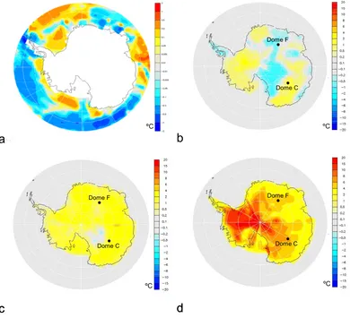
In order to investigate the robustness of the GENIE-1 ensem-bles, in particular with regard to the simplified atmosphere and snow models, we performed four equilibrium HadCM3 simulations. Hosing induces AMOC collapse and results in statistically significant warming of∼0.2–0.5◦C in summer (DJF) SST in the Weddell and Ross Seas (Fig. 5a), accom-panied by a reduction in Antarctic summer sea-ice extent and depth. A multi-model hosing ensemble (0.1 Sv, modern boundary conditions), performed to investigate inter-model uncertainty in response to hosing, also simulated warming in the Weddell Sea, apparently a consequence of enhanced deep convection and reduced sea ice (Stouffer et al., 2006).
In the absence of meltwater and ice-sheet forcing (Fig. 5b) HadCM3 fails to predict significant Antarctic SAT increase, though orbitally-forced summer warming of 3.0◦C is sim-ulated in Greenland. With freshwater hosing, precipitation-weighted SAT (Fig. 5c) increases by 2.2◦C at DOME F and 1.4◦C at DOME C, supporting GENIE-1 (annual-average East Antarctic warming of 1.6±1.0◦C). This warming is achieved after ∼100 years of the 200 year simulation. The removal of WAIS (Fig. 5d) increases the precipitation-weighted SAT anomaly to 4.9◦C at DOME F and to 5.0◦C at DOME C. Increased summer precipitation combines with greatest warming in summer when widespread West Antarc-tic snow melt is simulated. The HFWand HWAISsimulations
encompass observed WPT warming. As the GENIE-1 en-semble parameterisations were designed to provide an unbi-ased estimate of the uncertainty associated with large-scale processes, EFWand EWAISEast Antarctic SAT variability of
±1.0◦C and ±1.3◦C provide indicative lower-bound mea-sures of the parametric uncertainty in these single HadCM3 simulations.
4 Discussion
34 Figure 5
ab
c
d
ºC
ºC ºC
ºC
Dome F
Dome F Dome F
Dome C
Dome C Dome C
a
b
c
d
ºC
ºC ºC
ºC
Dome F
Dome F Dome F
Dome C
Dome C Dome C
Fig. 5. HadCM3 SST and SAT anomalies at 130 000 BP. (a) Southern summer freshwater-induced SST anomaly due to 1 Sv North Atlantic
hosing applied uniformly between 50–70◦N (HFW-HNFW). (b, c, d) Precipitation-weighted SAT anomalies relative to preindustrial (b) with no hosing (HNFW-HPI), (c) including hosing (HFW-HPI), (d) including hosing and with WAIS removed to land at 200 m (HWAIS-HPI).
substantial meltwater-forced WPTs (∼1.5◦C in this sin-gle parameterisation) at times which coincide closely with observed transient warming. We note that the tim-ing, magnitude and spatial distribution of the meltwater forcing is largely independent of the DOME F chronol-ogy (derived by tuning the O2/N2 ratio of trapped air
bubbles to 21 December insolation at 77◦S); the melt-water forcing is derived from an interpolation of the spa-tial distribution of Ice-4G onto the benthicδ18O stack (with an age model derived from a simple ice model driven by 21 June insolation at 65◦N).
ii) The TII ensembles provide a quantification of the un-certainty that arises from structural, parametric and boundary condition sources. The meltwater-induced collapse of Atlantic overturning leads to simulated East Antarctic warming at 128 500 BP (of 1.6±1.0◦C) to 0.5±1.0◦C above preindustrial. The ensemble av-eraged warming is consistent with Ganopolski and Roche (2009), who simulated∼1◦C and 2◦C
of∼4◦C (although 39 of 174 simulations exhibit
warm-ing greater than 2.5◦C above preindustrial); the full
reconciliation requires consideration of precipitation-weighted temperatures provided by the HadCM3 sim-ulations.
iii) The precipitation-weighted temperatures from the HadCM3 simulations allow a full reconciliation with observations, although this agreement is clearly associ-ated with considerable uncertainty arising from model (and observational) error sources and, notably, the de-gree of possible WAIS retreat. The HadCM3 hos-ing experiment (assumhos-ing modern WAIS) simulated precipitation-weighted temperatures in East Antarctica that are ∼2◦C warmer than preindustrial, consistent
with GENIE-1 and likely insufficient to reconcile with observations alone. We note that although maximum warming is achieved after∼100 years in this experi-ment (1 Sv hosing is applied throughout the 200 year simulation), CCSM3 hosing experiments in the LGM state indicated that warming in Antarctica shows the strongest relationship with the duration of the forcing rather than either rate or total volume of freshwater (Otto-Bliesner and Brady, 2010), so the possibility of additional simulated warming under prolonged hosing cannot be ruled out. Furthermore, the 200 year integra-tion neglects the transport of orbitally-driven warming of North Atlantic Deep Water to Circumpolar Deep Wa-ter (Duplessy et al., 2007) so that the simulated Antarc-tic temperature represents a lower bound. Cognisant of aforementioned uncertainties, the full reconciliation of HadCM3 with observations can be achieved under the assumption of WAIS retreat, with complete retreat producing precipitation-weighted temperature at both ice core sites (∼5◦C above preindustrial) that exceeds the generally accepted observed warming. The combi-nation of extensive temporal and parametric investiga-tions in GENIE-1 with detailed short-term integrainvestiga-tions of HadCM3, and the agreement between the two mod-els, substantially strengthens the conclusions that can be drawn from the experiments.
5 Summary and conclusions
In summary we have shown that GENIE-1 reproduces the temperature over Antarctica over the last 800 kyrs in a satis-factory way, with the notable exception of the last four inter-glacial periods. The three experiments we have performed, with GENIE-1 and HadCM3, together enable us to postu-late that by including processes represented in both models and accounting for the statistical distribution of responses we could explain both the timing and magnitude of obser-vations through the introduction of meltwater forcing during terminations, likely amplified by feedbacks resulting from WAIS retreat, though at present we are not able to achieve
this in a single model. Although the tails of both meltwater-forced ensemble distributions (EFW and EWAIS)encompass
observed WPT warming, reconciliation of data and mod-elling can only be readily achieved under the assumption of WAIS retreat. The combination of freshwater hosing and WAIS forcing produces precipitation-weighted temperatures ∼5◦C above preindustrial in HadCM3. This warming arises from the combined effects of increased East Antarctic tem-perature and summer precipitation. We do not conclude that complete WAIS retreat is necessary to explain the model-data discrepancy, but have applied the extreme boundary condi-tions of modern and absent WAIS to span the possible range of the forcing associated with this feedback. We are not aware of other potential feedbacks that might explain∼4◦C warming across East Antarctica.
Our simulations neglect possible convection feedbacks driven by WAIS meltwater which would be expected to re-duce Antarctic temperature. The magnitude of this neglected feedback (∼0.5◦C reduction in Antarctic SAT, c.f. Swinge-douw et al., 2009) compares to ensemble-averaged Antarctic bipolar warming of 1.6±1.0◦C (assuming no WAIS retreat). We note that the full magnitude of this feedback would im-ply a significant loss of WAIS ice. Assuming WAIS retreat would have occurred late in the termination, a feedback of this magnitude would not be inconsistent with “cooling re-bounds” that are observed during the later stages of recent terminations (Cortese et al., 2007), though we note the pos-sibility that such cooling events could alternatively be ex-plained as a consequence of the reorganisation of the ocean circulation after the cessation of meltwater.
Several other points in the DOME F record are sugges-tive of a meltwater-forced bipolar signal, in particular the three anomalously warm interstadials which were apparently cooler at DOME C. During the previous three terminations, the bipolar seesaw would have warmed Antarctica through-out the deglaciation, with WAIS retreat occurring at some point, presumably late in the termination as interglacial con-ditions were approached. In contrast, the resumption of over-turning during the Bølling-Allerød/ACR cooled Antarctica towards the end of TI, potentially preventing further south-ern warming through stabilisation of the WAIS.
Acknowledgements. We would like to thank the three anonymous
referees. Their careful and extensive comments have resulted
in a much improved and clarified manuscript. This work was
funded by the UK Natural Environment Research Council through QUEST-DESIRE (NE/E007600/1).
References
Barker, S., Diz, P., Vautravers, M. J., Pike, J., Knorr, G., Hall, I. R., and Broecker, W. S.: Interhemispheric Atlantic seesaw response during the last deglaciation, Nature, 457, 1097–1103, 2009. Berger, A.: Long term variations of caloric insolation resulting from
the Earth’s orbital elements, Quaternary Res., 9, 139–167, 1978. Bintanja, R., van de Wal, R. S. W., and Oerlemans, J.: Modelled at-mospheric temperatures and global sea-levels over the past mil-lion years, Nature, 437, 125–128, 2005.
Blunier, T., Chappellaz, J., Schwander, J., D¨allenbach, A., Stauf-fer, B., Stocker, T. F., Raynaud, D., Jouzel, J., Clausen, H. B., Hammer, C. U., and Johnsen, S. J.: Asynchrony of Antarctic and Greenland climate change during the last glacial period, Nature, 394, 739–743, 1998.
Carlson, A. E.: Why there was not a Younger Dryas-like event dur-ing the Penultimate Deglaciation, Quaternary Sci. Rev., 27, 882– 887, 2008.
Cheng, H., Edwards, R. L., Wang, Y., Kong, X., Ming, Y., Kelly, M. J., Wang, X., Gallup, C. D., and Liu, W.: A penultimate glacial monsoon record from Hulu Cave and two-phase glacial termina-tions, Geology, 34, 217–220, 2006.
Cheng, H., Edwards, R. L., Broecker, W. S., Denton, G. H., Kong, X., Wang, Y., Zhang, R., and Wang, X.: Ice age terminations, Science, 326, 248–251, 2009.
Cortese, G., Abelmann, A., and Gersonde, R.: The last five glacial-interglacial transitions: a high resolution 450,000-year record from the subantarctic Atlantic, Paleoceanography, 22, PA4203, doi:10.1029/2007PA001457, 2007.
Dansgaard, W., Johnsen, S. J., Clausen, H. B., Dahl-Jensen, D., Gundestrup, N. S., Hammer, C. U., Hvldberg, C. S., Steffensen, J. P., Svelnbj¨ornsdottir, A. E., Jouzel, J., and Bond, G.: Evidence for general instability of past climate from a 250-kyr ice-core record, Nature, 364, 218–220, 1993.
Delmotte, M., Chappellaz, J., Brook, E., Yiou, P., Barnola, J. M., Goujon, C., Raynaud, D., and Lipenkov, V. I.: Atmospheric methane during the last four glacial-interglacial cycles: rapid changes and their link with Antarctic temperature, J. Geophys. Res., 109, D12104, doi:10.1029/2003JD004417, 2004.
Duplessy, J. C., Roche, D. M., and Kageyama, M.: The deep ocean during the last interglacial period, Science, 316, 89–91, 2007. Edwards, N. R. and Marsh, R.: Uncertainties due to
transport-parameter sensitivity in an efficient 3-D ocean-climate model, Clim. Dynam., 24, 415–433, 2005.
Ganopolski, A. and Rahmstorf, S.: Rapid changes of glacial cli-mate simulated in a coupled clicli-mate model, Nature, 409, 153– 158, 2001.
Ganopolski, A. and Roche, D.: On the nature of lead-lag relation-ships during glacial-interglacial climate transitions, Quaternary Sci. Rev., 28, 3361–3378, 2009.
Gordon, C., Cooper, C., Senior, C. A., Banks, H., Gregory, J. M., Johns, T. C., Mitchell, J. F. B., and Wood, R. A.: The simulation of SST, sea ice extents and ocean heat transports in a version of the Hadley Centre coupled model without flux adjustments, Clim. Dynam., 16, 147–168, 2000.
Groll, N., Widmann, M., Jones, J. M., Kaspar, F., and Lorenz, S. J.: Simulated relationships between regional temperatures and large-scale circulation: 125 kyr BP (Eemian) and the preindus-trial period, J. Climate, 18, 4032–4045, 2005.
Holden, P. B., Edwards, N. R., Oliver, K. I. C., Lenton, T. M., and
Wilkinson, R. D.: A probabilistic calibration of climate sensi-tivity and terrestrial carbon change in GENIE-1, Clim. Dynam., doi:10.1007/s00382-009-0630-8, in press, 2010.
Huybrechts, P. and de Wolde, J.: The dynamic response of the Greenland and Antarctic ice sheets to multiple-century climate warming, J. Climate, 8, 2169–2188, 1999.
Jouzel, J., Masson-Delmotte, V., Cattani, O., Dreyfus, G., Falourd, S., Hoffman, G., Minster, B., Nouet, J., Barnola, J. M., Chappel-laz, J., Fischer, H., Gallet, J. G., Johnsen, S., Leuenberger, M., Loulergue, L., Luethi, D., Oerter, H., Parrenin, F., Raisbeck, G., Raynaud, D., Schilt, A., Schwander, J., Selmo, E., Souchez, R., Spahni, R., Stauffer, B., Steffensen, J. P., Stenni, B., Stocker, T. F., Tison, J. L., Werner, M., and Wolff, E. W.: Orbital and Mil-lennial Antarctic climate variability over the past 800 000 years, Science, 317, 793–796, 2007.
Kawamura, K., Parrenin, F., Lisiecki, L. Uemura, R., Vimeux, F., Severinghaus, J. P., Hutterli, M. A., Nakazawa, T., Aoki, S., Jouzel, J., Raymo, M., Matsumoto, K., Nakata, H., Motoyama, H., Fujita, S., Goto-Azuma, K., Fujii, Y., and Watanabe, O.: Northern Hemisphere forcing of climatic cycles in Antarctica over the past 360,000 years, Nature, 448, 912–916, 2007. Kelly, M. J., Edawrds, R. L., Cheng, H., Yuan, D., Cai, Y., Zhang,
M., Lin, Y., An, Z.: High resolution characterisation of the Asian Monsoon between 146,000 and 99,000 years B.P. from Donge Cave, China and global correlation of events surrounding Termi-nation II, Palaeogeogr. Palaeocl., 236, 20–38, 2006.
Kopp, R. E., Simons, F. J., Mitrovica, J. X., Maloof A. C., and Oppenheimer, M.: Probabilistic assessment of sea level during the last interglacial stage, Nature, 462, 863–868, 2009.
Lenton, T. M., Williamson, M. S., Edwards, N. R., Marsh, R., Price, A. R., Ridgwell, A. J., Shepherd, J. G., Cox, S. J., and The GE-NIE team: Millennial timescale carbon cycle and climate change in an efficient Earth system model, Clim. Dynam., 26, 687–711, 2006.
Lisiecki, L. E. and Raymo, M. E.: A Pliocene-Pleistocene stack of 57 globally distributed benthicδ18O records, Paleoceanography, 20, PA1003, doi:10.1029/2004PA001071, 2005.
Loulergue, L., Schilt, A., Spahni, R., Masson-Delmotte, V., Blunier, T., Lemieux, B., Barnola, J.-M., Raynaud, D., Stocker, T. F., and Chappellaz, J. M.: Orbital and millennial scale features of atmo-spheric CH4over the last 800,000 years, Nature, 453, 383–386, 2008.
Luethi, D., Le Floch, M., Bereiter, B., Bluner, T., Barnola, J.-M., Siegenthaler, U., Raynaud, D., Jouzel, J., Fischer, H., Kawamura, K., and Stocker, T. F.: High-resolution carbon dioxide concentra-tion record 650,000–800,000 years before present, Nature, 453, 379–382, 2008.
Lunt, D. J., Williamson, M. S., Valdes, P. J., Lenton, T. M., and Marsh, R.: Comparing transient, accelerated, and equilibrium simulations of the last 30,000 years with the GENIE-1 model, Clim. Past, 2, 221–235, doi:10.5194/cp-2-221-2006, 2006. Marsh, R., Yool, A., Lenton, T. M., Gulamali, M. Y., Edwards,
N. R., Shepherd, J. G., Krznaric, M., Newhouse, S., and Cox, S. J.: Bistability of the thermohaline circulation identified through comprehensive 2-parameter sweeps of an efficient cli-mate model, Clim. Dynam., 23, 761–777, 2004.
Johnsen, S., R¨othlisberger, R., Hansen, J., Mikolajewicz, U.,
and Otto-Bliesener, B.: EPICA Dome C record of glacial
and interglacial intensities, Quaternary Sci. Rev., 29, 113–128, doi:10.1016/j.quascirev.2009.09.030, 2010.
McManus, J. F, Oppo, D. W., and Cullen, J. L.: A 0.5 million year record of millennial-scale climate variability in the North Atlantic, Science, 283, 971–976, 1999.
McManus, J. F., Francois, R., Gherardi, J.-M., Keigwin, L. D., and Brown-Leger, S.: Collapse and rapid resumption of Atlantic meridional circulation linked to deglacial climate changes, Na-ture, 428, 834–837, 2004.
Montoya, M., von Storch, H., and Crowley, T. J.: Climate simu-lation for 125 kyr BP with a coupled ocean-atmosphere general circulation model, J. Climate, 13, 1057–1072, 2000.
Nuernberg, C. C., Bohrmann, G., and Schlueter, M.: Barium ac-cumulation in the Atlantic sector of the Southern Ocean: re-sults from 190,000 year records, Paleoceanography, 12, 594– 603, 1997.
Otto-Bliesner, B. L., Marshall, S. J., Overpeck, J. T., Miller, G. H., Hu, A., and CAPE Last Interglacial Project Members: Simulat-ing Arctic climate warmth and icefield retreat in the last inter-glaciation, Science, 311, 1751–1753, 2006.
Otto-Bliesner, B. L. and Brady, E. C.: The sensitivity of the climate response to the magnitude and location of freshwater forcing: last glacial maximum experiments, Quaternary Sci. Rev., 29, 56– 73, 2010.
Overpeck, J. T., Otto-Bliesner, B. L., Miller, G. H., Muhs, D. R., Alley, R. B., and Kiehl, J. T.: Paleoclimatic evidence for future ice-sheet instability and rapid sea-level rise, Science, 311, 1747– 1750, 2006.
Peltier, W. R.: Ice age paleotopography, Science, 265, 195–201, 1994.
Peltier, W. R.: Global glacial isostasy and the surface of the ice-age earth: the ICE-5G (VM2) model and GRACE, Annu. Rev. Earth Pl. Sc., 32, 111–149, 2004.
Pollard, D. and DeConto, R. M.: Obliquity-paced Pliocene West Antarctic ice sheet oscillations, Nature, 457, 329–333, 2009. Rignot, E. and Jacobs, S. S.: Rapid bottom melting widespread near
Antarctic ice sheet grounding lines, Science, 296, 2020–2023, 2002.
Rougier, J.: Probabilistic inference for future climate using an en-semble of climate model evaluations, Clim. Change, 81, 247– 264, 2007.
Schneider von Deimling, T., Ganopolsky, A., Held, H., and Rahm-storf, S.: How cold was the last glacial maximum, Geophys. Res. Lett., 33, L14709, doi:10.1029/2006GL026484, 2006.
Sime, L. C., Wolff, E. W., Oliver, K. I. C., and Tindall, J. C.: Ev-idence for warmer interglacials in East Antarctic ice cores, Na-ture, 462, 342–345, 2009.
Stocker, T. F. and Johnsen, S. F.: A minimum thermodynamic model for the bipolar seesaw, Paleoceanography, 18, 1087, doi:10.1029/2003PA000920, 2003.
Stocker, T. F., Timmermann, A., Renold, M., and Timm, O.: Ef-fects of salt compensation on the climate model response in sim-ulations of large changes of the Atlantic Meridional Overturning Circulation, J. Climate, 20, 5912–5928, 2007.
Stouffer, R. J., Yin, J., Gregory, J. M., Dixon, K. W., Spelman, M. J., Hurlin, W., Weaver, A. J., Eby, M., Flato, G. M., Hasumi, H., Hu, A., Jungclaus, J. H., Kamenkovich, I. V., Levermann, A., Montoya, M., Murakami, S., Nawrath, S., Oka, A., Peltier, W. R., Robitaille, D. Y., Sokolev, A., Vettoretti, G., and Weber, S. L.: Investigating the causes of the response of the thermohaline circulation to past and future climate changes, J. Climate, 19, 1365–1387, 2006.
Swingedouw, D., Fichefet, T., Goosse, H., and Loutre, M. F.: Im-pact of transient freshwater releases in the Southern Ocean on the AMOC and climate, Clim. Dynam., 33, 365–381, 2009. Thomas, A. L., Henderson, G. M., Deschamps, P., Yokoyama, Y.,
Mason, A. J., Bard, E., Hamelin, B., Durand, N., and Camoin, G.: Penultimate deglacial sea-level timing from uranium/thorium dating of Tahitian corals, Science, 324, 1186–1189, 2009. Venz, K. A., Hodell, D. A., Stanton C., and Warnke D. A.: A 1.0
Myr record of Glacial North Atlantic Intermediate Water vari-ability from ODP site 982 in the northeast Atlantic, Paleoceanog-raphy, 14, 42–52, 1999.
Wang, Y. J., Cheng, H., Edwards, R. L., An, Z. S., Wu, J. Y., Shen, C.-C., and Dorale, J. A.: A high-resolution absolute dated Late Pleistocene monsoon record from Hulu Cave, China, Science, 294, 2345–2348, 2001.
Weaver, A. J., Saenko, O. A., Clark, P. U., and Mitrovica, J. X.: Meltwater Pulse 1A from Antarctica as a trigger of the Bølling-Allerød warm interval, Science, 299, 1709–1713, 2003. Williamson, M. S., Lenton, T. M., Shepherd, J. G., and Edwards,
N. R.: An efficient terrestrial scheme (ENTS) for Earth system modelling, Ecol. Model, 198, 362–374, 2006.
Wolff, E. W., Fischer, H., and R¨othlisberger, R.: Glacial termi-nations as southern warmings without northern control, Nat. Geosci., 2, 206–209, 2009.