www.atmos-meas-tech.net/9/5007/2016/ doi:10.5194/amt-9-5007-2016
© Author(s) 2016. CC Attribution 3.0 License.
Microphysical particle properties derived from inversion algorithms
developed in the framework of EARLINET
Detlef Müller1, Christine Böckmann2, Alexei Kolgotin3, Lars Schneidenbacha, Eduard Chemyakin4, Julia Rosemann2, Pavel Znak5, and Anton Romanov6
1School of Physics, Astronomy and Mathematics, University of Hertfordshire, Hatfield, Hertfordshire, UK 2Institute of Mathematics, University of Potsdam, Am Neuen Palais 10, 14469 Potsdam, Germany 3Physics Instrumentation Center, Troitsk, Russia
4Science Systems and Applications, Inc., NASA Langley Research Center, Hampton VA, USA
5V. A. Fock Institute of Physics, St. Petersburg University, Ulyanovskaya 1, 198504 St. Petersburg, Russia 6The National University of Science and Technology, Moscow, Russia
aformerly at: Institute for Computer Science, University of Potsdam, Am Neuen Palais 10,
14469 Potsdam, Germany
Correspondence to:Detlef Müller ([email protected])
Received: 24 August 2015 – Published in Atmos. Meas. Tech. Discuss.: 8 December 2015 Revised: 20 May 2016 – Accepted: 10 June 2016 – Published: 12 October 2016
Abstract. We present a summary on the current status of two inversion algorithms that are used in EARLINET (Eu-ropean Aerosol Research Lidar Network) for the inversion of data collected with EARLINET multiwavelength Raman lidars. These instruments measure backscatter coefficients at 355, 532, and 1064 nm, and extinction coefficients at 355 and 532 nm. Development of these two algorithms started in 2000 when EARLINET was founded. The algorithms are based on a manually controlled inversion of optical data which allows for detailed sensitivity studies. The algorithms allow us to derive particle effective radius as well as volume and surface area concentration with comparably high confidence. The re-trieval of the real and imaginary parts of the complex refrac-tive index still is a challenge in view of the accuracy required for these parameters in climate change studies in which light absorption needs to be known with high accuracy. It is an extreme challenge to retrieve the real part with an accuracy better than 0.05 and the imaginary part with accuracy bet-ter than 0.005–0.1 or±50 %. Single-scattering albedo can be computed from the retrieved microphysical parameters and allows us to categorize aerosols into high- and low-absorbing aerosols.
On the basis of a few exemplary simulations with synthetic optical data we discuss the current status of these manually operated algorithms, the potentially achievable accuracy of
data products, and the goals for future work. One algorithm was used with the purpose of testing how well microphysi-cal parameters can be derived if the real part of the complex refractive index is known to at least 0.05 or 0.1. The other algorithm was used to find out how well microphysical pa-rameters can be derived if this constraint for the real part is not applied.
The optical data used in our study cover a range of Ångström exponents and extinction-to-backscatter (lidar) ra-tios that are found from lidar measurements of various aerosol types. We also tested aerosol scenarios that are con-sidered highly unlikely, e.g. the lidar ratios fall outside the commonly accepted range of values measured with Ra-man lidar, even though the underlying microphysical parti-cle properties are not uncommon. The goal of this part of the study is to test the robustness of the algorithms towards their ability to identify aerosol types that have not been measured so far, but cannot be ruled out based on our current knowl-edge of aerosol physics.
7–10 µm in our simulations where the Potsdam algorithm is limited to the lower value. We considered optical-data errors of 15 % in the simulation studies. We target 50 % uncertainty as a reasonable threshold for our data products, though we at-tempt to obtain data products with less uncertainty in future work.
1 Introduction
The start of EARLINET (European Aerosol Research Li-dar Network) in 2000 marked the beginning of the devel-opment of inversion algorithms that can be used for the re-trieval of aerosol microphysical properties from Raman li-dar observations. Based on exploratory work (Qing et al., 1989) it seemed feasible that Raman lidar measurements of backscatter coefficients and extinction coefficients could pro-vide variables such as particle effective radius and complex refractive index from which, under favourable measurement conditions, single-scattering albedo could be derived.
We followed two conceptual approaches. One methodol-ogy was developed at the Leibniz Institute for Tropospheric Research (TROPOS), Leipzig, Germany. The development of the methodology continues at the University of Hertford-shire (UH). The second method was developed at the Uni-versity of Potsdam (UP) (Potsdam, Germany). Both methods in part follow the same basic mathematical concepts in the sense that they are true inversion algorithms. True inversion algorithms mean the following: (a) the underlying mathemat-ical equations that connect the microphysmathemat-ical particle prop-erties (which are the variables we are interested in) and the optical properties (which are the variables that are measured with lidar) are solved explicitly; (b) therefore we do not carry out forward computations, which are commonly referred to as Mie-scattering computations; (c) we do not use traditional look-up tables that contain an array of microphysical aerosol properties and the optical properties that belong to these mi-crophysical properties; and (d) our approach neglects con-straints that are used in forward computations, for example the need to prescribe the shape of the particle size distribu-tion as input.
The advantage of our approach is that we can identify the share of fine-mode and coarse-mode particles in particle size distributions, as the inversion algorithms allow us to find ap-proximate solutions of the underlying particle size distribu-tions. As with any other method, there exists plenty of dis-advantages, for example measurement errors have a direct impact on the quality of the retrieval results. If measurement errors become too large, the inversion algorithms will not be able to find reasonable solutions. The inversion algorithms also respond strongly to systematic errors of the optical in-put data. This means that if calibrations of the optical profiles are not done carefully, or if optical data are faulty because of the incomplete overlap between laser beam and field-of-view
of the receiver telescope (Wandinger and Ansmann, 2002), the inversion algorithms will deliver the wrong microphysi-cal particle properties.
1.1 Work at TROPOS/UH
With regard to work at TROPOS/UH, our algorithm devel-opment began on the basis of data we obtained from the first truly operational multiwavelength Raman lidar (Althausen et al., 2000) in the 1990s. This instrument provides backscat-ter coefficients measured at 355, 400, 532, 710, 800, and 1064 nm and extinction coefficients at 355 and 532 nm. The system uses four lasers that operate simultaneously. The high costs of this system and the labour-intensive measurement and data analysis work showed us fairly early that a wider use of the inversion technology in the lidar community would require reducing the optical data needed for data inversion. Based on exploratory work (Müller et al., 2001b; Veselovskii et al., 2002; Böckmann et al., 2005), it seemed feasible that a Raman lidar consisting of only one Nd:YG laser could still fulfil the minimum number of optical data such that suc-cessful data inversion could be carried out. This minimum requirement is measurements of backscatter coefficients at 355, 532, and 1064 nm and extinction coefficients at 355 and 532 nm.
The algorithm that was initially developed at TROPOS fol-lows the concept of Tikhonov’s inversion with regularization (Tikhonov and Arsenin, 1977). The algorithm is based on a data-operator-controlled software environment. That makes this algorithm highly labour-intensive and the output with regard to inversion results is rather low. However, this ap-proach allows us to carry out detailed sensitivity studies in order to test the quality of the data inversion products and to push the envelope in what can theoretically be achieved in terms of aerosol characterization with state-of-the-art mul-tiwavelength Raman lidar. Several sensitivity studies dealt with the ability of the algorithm to retrieve effective radius, and surface area and volume concentration, and the com-plex refractive index (CRI) (Müller et al., 1999a, b, 2001b; Veselovskii et al., 2002, 2004). Most sensitivity studies dealt with monomodal particle size distributions, although some work has also been done in the context of bimodal particle size distributions (Veselovskii et al., 2004).
The retrieval of the CRI remains a major challenge in our work. The accuracy requirements for the imaginary part of the CRI are considerable if we want to obtain useful values (high accuracy and precision) of the single-scattering albedo (SSA) which is one of the key parameters in climate change studies. Mishchenko et al. (2004) mention that an accuracy of 0.03 and a precision of 0.02 of the SSA in the wavelength range between 350 and 2500 nm is needed in order to meet the requirements for sensible impact studies of particulate pollution on radiative forcing.
data-operator-controlled data analysis which involves a careful evaluation of the inversion results (particularly of the CRI). We learnt to retrieve the imaginary part to its correct order of magnitude if it is less than 0.01i. This value describes moderately light-absorbing aerosol. We learnt to keep the uncertainty bars to approximately ±50 % if the imaginary part is larger than 0.01i. Such values describe strongly light-absorbing parti-cles. We noticed that a systematic bias of the imaginary part may occur if its value is close to 0. This bias is naturally in-troduced as the imaginary part has a minimum value of 0. This lower limit leads to an underestimation of the SSA.
We analysed plenty of different aerosol types in the course of more than 15 years of measurements with multiwave-length Raman lidar. Still, a statistically significant set of re-sults for each aerosol type has not been achieved because of the labour-intensive manual data analysis. Examples of aerosol types we analysed involve urban/industrial pollution over Europe (Müller et al., 2005), East Asia (Noh et al., 2011), and South Asia (Müller et al., 2001a). We investi-gated properties of fresh and aged biomass burning aerosols produced in North America (Müller et al., 2005), Europe (Alados-Arboledas et al., 2011), and West Africa (Tesche et al., 2011). In all these cases we assumed in our data anal-ysis that particles have spherical shape, i.e. we used Mie the-ory in our simulations.
We remain cautious with regard to the inversion of opti-cal data that describe non-spheriopti-cal (mineral dust) particles, as to date we do not have a reliable light-scattering model that allows us to describe light-scattering at 180◦. We car-ried out some limited studies in which we used the T-matrix algorithm for non-spherical (spheroid) particles as a test on how far we can use this model which has not been designed for describing particle backscatter coefficients. We conclude from our limited set of studies that we may be able to in-fer particle effective radius of dust particles and the ratio of spherical-to-non-spherical particles (Veselovskii et al., 2010; Müller et al., 2013), though doubt regarding the trustworthi-ness of the results remains. We fail in retrieving sensible re-sults with regard to the complex refractive index.
1.2 Work at UP
The Potsdam algorithm that was developed at UP is based on the concept of using truncated singular value decomposi-tion (TSVD) as regularizadecomposi-tion method, (e.g. Hansen (2010)). This method was adapted to work for the retrieval of the particle size distribution function (PSD) and is called hy-brid regularization technique (Böckmann, 2001) since it is using a triple of regularization parameters. Simulation stud-ies demonstrated that the hybrid method can be used to invert monomodal and bimodal PSDs (Böckmann, 2001; Böck-mann et al., 2005). The minimum requirement for mean-ingful inversion results are optical input data obtained from measurements of backscatter coefficients at 355, 532, and 1064 nm and extinction coefficients at 355 and 532 nm.
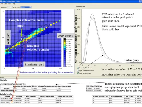
How-ever, the software can also be used with a smaller or larger number of optical coefficients. The inversion of an ill-posed problem, such as the retrieval of the PSD, is always a chal-lenging task because small measurement errors and tiny rounding errors often will be hugely amplified during the so-lution process unless an appropriate regularization method is used. The use of a regularization method requires the careful determination of the associated regularization param-eters (e.g. Doicu et al. (2010); Hansen (2010); Rodgers (2000); Vogel (2002)). Therefore, in one of the next stages of our development work we decided to use two regularization techniques in parallel for comparison purposes. The second method we used for comparison is an iterative regulariza-tion method based on Páde iteraregulariza-tion (Kirsche and Böckmann, 2006; Böckmann and Pornsawad, 2008). Here, the number of iteration steps serves as the regularization parameter. This method was adapted and tested successfully to invert the PSD (Böckmann and Kirsche, 2006). The approximated PSD is a linear combination of B splines with appropriately deter-mined weights. The B splines of orderd are polynomials of degreed−1. Since the distribution of the B-spline nodes also plays a critical role, we modified the first algorithm TSVD such that non-equidistant node grids can be used too (Böck-mann, 2001). The iterative method was equipped with an adaptive non-equidistant node grid by Osterloh et al. (2011). There is another challenge that needs to be considered. The CRI is actually also unknown. In order to solve this problem, a grid of viable options for the CRI (all combinations of real parts of CRI (RPCRI) and imaginary parts of CRI (IPCRI)) is assumed. If this is not done, one additionally has to deal with a non-linear problem. The CRI grid technique is very time consuming, i.e. the computer runtime of the inversion pro-cess is very large. Therefore, we developed a semi-automated software for spherical particles which is able to run on a par-allel processor machine (Osterloh et al., 2009) (see Fig. 1). The software is adapted with a tool that reads NetCDF files from the EARLINET database (The EARLINET publishing group, 2014).
Figure 1.Screen shot of the developed software and explanation of the post-processing procedure: selection of suitable grid points of CRI clustering along the diagonal domain (left), corresponding PSD and initial PDS (right), and tables with retrieved microphysical parameters for each selected CRI and mean values with standard deviation (bottom). The residual errors on the right hand side of the grid appear in ascending order from top to bottom on a logarithmic scale.
and extinction coefficient profiles, as well as depolarization ratio information.
The semi-automatic software was applied to measurement cases. We analysed Raman lidar measurement data with three backscatter coefficients at 355, 532, and 1064 nm and two extinction coefficients at 355 and 532 nm. From these op-tical particle variables we retrieved microphysical particle properties of different aerosol types. Successful retrievals have been made for biomass burning and industrial pollu-tion aerosols over Germany (Wandinger et al., 2002), conti-nental aerosols (Eixmann et al., 2002), Arctic haze aerosols (Hoffmann et al., 2012), biomass burning aerosols over Ro-mania (Osterloh et al., 2013) and Athens (Papayannis et al., 2008). Moreover, the two-dimensional spheroidal model was applied to a measurement scenario of Saharan dust observed over Barbados (13.16◦N, 59.44◦W). We obtained results for the two-dimensional fine-mode PSD. We found promising
results, in particular, when we used additional depolarization ratio profiles (Böckmann et al., 2012). Finally, Samaras et al. (2015) show a direct quantitative comparison of the retrieved microphysical properties to measurements from a Compact Time of Flight Aerosol Mass Spectrometer (AMS) which al-lowed us to validate the results from our algorithm for the case of spherical particles. With regard to the fine-mode frac-tion of the investigated PSD, we observed remarkable simi-larities between the retrieved PSD and the one measured by the AMS. Additionally, microphysical retrievals performed with Sun photometer data were also used to explore the re-sults of biomass burning aerosols.
of both algorithms in future rather than selecting one algo-rithm over the other algoalgo-rithm in EARLINET. We carried out simulations with the main purpose of investigating what maximum accuracy and precision of microphysical param-eters can be achieved (UP algorithm). The complex refrac-tive index is the key to retrieving accurate values of single-scattering albedo and profiles of absorption coefficients. We therefore investigated if an accurate knowledge of the real part of the refractive index would significantly improve the retrieval of the imaginary part which then would feed into improved values of single-scattering albedo. We used the UH/TROPOS algorithm for this part of the study.
Section 2 presents main features of the two methodologies. Section 3 presents some simulation studies that illustrate the current status. Section 4 closes with a summary and outlook.
2 Methodology
The microphysical properties are derived from solving Fred-holm integral equations of the first kind (Müller et al., 1999a; Veselovskii et al., 2002; Böckmann, 2001; Böckmann et al., 2005; Ansmann and Müller, 2005). These equations can be written in general terms as
gl∗(λi)=
∞
Z
0
Kl(m, r, λi, s) f∗(r)dr. (1)
The termgl∗(λi)denotes the exact optical data at the mea-surement wavelength λi. The optical data usually have an uncertainty as we use experimental data. The subscriptl de-notes the type of optical data, i.e.βdenotes particle backscat-ter coefficients andαdenotes particle extinction coefficients. The backscatter and extinction kernel functions are de-noted byKβ(m, r, λ, s)andKα(m, r, λ, s). The kernel func-tions depend on the complex refractive indexmof the parti-cles, i.e.m = mR−mIi. The termmRdenotes the real part.
The termmIidenotes the imaginary part of the CRI. The
ra-dius of the particles is denoted asr. The shape propertiessof the particles determine their backscatter and extinction prop-erties. We only consider spherical shape of the particles and therefore drop this parameter in the following discussion.
The kernel functionsKl(m, r, λi)are calculated from Mie-scattering theory (Bohren and Huffman, 1983). The term f∗(r) describes the exact (true) particle size distribution which is described as the number of particles per unit vol-ume between particle radiusrandr+dr.
Equation (1) can be written as
gp∗=
rmax Z
rmin
Kp(m, r) f∗(r)dr+plimits. (2)
The term gp∗ describes the exact values of the optical data. The subscriptp=(l, λi)describes the kind of optical input
data at a given wavelength. The lower and upper integration limits of the particle radii within which the inversion is per-formed are denoted byrminandrmax. We write this radius
interval as [rmin, rmax]. The termplimitsrepresents the model error that results from the fact that the integration limits are not from 0 to∞.
Disregarding the model error term we obtain
gp∗=
rmax Z
rmin
Kp(m, r) fM(r)dr . (3)
The investigated PSDfM(r)is obtained from the
numer-ical solution of Eq. (3) (Twomey, 1965; Zuev and Naats, 1983; Engl et al., 1996; Hansen, 2010). The numerical solu-tion is not an easy task since this compact Fredholm operator is ill posed. Firstly, the expressionfM(r)is approximated by
a sum that consists of the linear superposition of base func-tions:
fM(r)=f (r)+ (r)=
NB
X
j=1
fjBj(r)+ (r) . (4)
The termf (r)is an approximation of the solution of Eq. (3). The expressionfj describes weight coefficients.Bj(r)are B-spline base functions. NBis the number of base functions
that are used in the inversion. The term (r)is the discretiza-tion error. This error is caused by discretizing the PSD with the linear combination of base functions.
Neglecting the discretization error term we can express the measured optical particle properties gp by an approxi-mation of a linear combination of base functions according to Eqs. (3) and (4):
gp=
NB
X
j=1
Apj(m) fj. (5)
The matrix elementsApjare calculated from the kernel func-tions and the base funcfunc-tions as
Apj= rmax
Z
rmin
Kp(m, r) Bj(r)dr . (6)
If we write the optical data as vector g = gp and the weight coefficients as vectorf =fjwe can write Eq. (5) as a vector–matrix expression:
g = Af. (7)
The matrixA=
The unknown vector of the weight coefficients f is con-nected by the matrix operatorAwith the optical data vector
g. We note that the data vectorgcontains measurement er-rors. For ill-conditioned systems this means that small data errors may be amplified strongly during a standard solution process. Finally, the total error contains the measurement er-ror and the mathematical approximation erer-rors in an additive way.
The TROPOS/UH algorithm and the UP algorithm use dif-ferent regularization methods. The TROPOS/UH algorithm uses Tikhonov regularization (Phillips, 1962; Tikhonov and Arsenin, 1977). The UP algorithm uses regularization on the basis of truncated singular value decomposition (TSVD) (Engl et al., 1996; Hansen, 2010).
With respect to the subsequently realized simulation study in which we apply simulated noise to the optical data, the following issue is considered. On the one hand, since noise or measurement errors are randomly distributed to the opti-cal data one needs a reasonable sample size for the simula-tion study for the case of noisy data. On the other hand, the simulation studies are very time consuming. Thus, a compro-mise between reasonable sample size and runtime is needed. Therefore, we decided on 8–10 runs as sample size. Details of both algorithms are described in the next subsections.
2.1 TROPOS/UH algorithm
2.1.1 Solving the Fredholm equations
Detailed descriptions of solving the modified version of Tikhonov’s inversion algorithm is explained in detail by Müller et al. (1999a) and Veselovskii et al. (2002).
The number of base functions, NB, is equal to or exceeds
the number of optical data. Veselovskii et al. (2002, 2004) prefer to keep the number of base functions nearly equal to the number of input optical data.
In the case of the algorithm developed at TROPOS, the base functions have triangular shape on a logarithmic ra-dius scale (Müller et al., 1999a, b). We tested two other shapes of base functions, i.e. histogram columns (Heintzen-berg et al., 1981) and monomodal logarithmic-normal distri-butions (Amato et al., 1995). We did not find significant im-provement of our data products when we used these shapes of base functions. We believe that one main cause for this re-sult is the fact that the main error sources in data inversion are incorrect optical input data, unknown complex refractive index and uncertainties caused by the regularization proce-dure. All these errors outweigh the potential improvements that could be obtained by using a more suitable description of the investigated PSDs, e.g. base functions of logarithmic-normal shape. The base functions of second order, i.e. first degree that we use, have also shown to work sufficiently well for the reconstruction of PSDs of bimodal shape (Veselovskii et al., 2004).
We can solve Eq. (7) by introducing the transposed matrix AT. Assuming its existence we use ATA−1as the inverse of matrixATA. In that way we obtain the simple normal so-lution of Eq. (7) for the weight factors:
f= ATA−1
ATg. (8)
The solution of Eq. (8) usually leads to physically useless re-sults because the mathematical problem is ill posed. The rea-son for it is that the matrix-operatorAis ill conditioned since it is the discretized representative of an infinite-dimensional ill-posed operator. Details on this property can be found in, e.g. Twomey (1977). Explanations can also be found in, e.g. Müller et al. (1999a), who provide details on how to overcome this problem. Briefly, we introduce the equation (Twomey, 1977; Tikhonov and Arsenin, 1977)
ATA+γHf=ATg. (9)
The expression H is the smoothing matrix operator (Twomey, 1977). This operator describes the physical con-straint that the retrieved PSD does not show ”large” oscilla-tions in the size range for which the PSD is retrieved. This size range is determined by the inversion window.
Details on the appropriate choice of Hcan be found in Twomey (1977).Hinfluences the maximum difference be-tween the weight factors of successive base functions.γ is the Lagrange multiplier. It is the non-negative regularization parameter that determines the degree of smoothing of the in-vestigated PSDs, i.e. the strength of the operatorH.
2.1.2 Identification of the solution space
Finding the solution requires the application of several con-straints. These constraints stabilize the inversion problem and help us reject mathematical solutions that are physi-cally not reasonable. We use the simplifying assumption of a wavelength- and size-independent complex refractive index of the aerosol particles.
The rationale for using a gliding inversion window is given by Müller et al. (1999a, b). We used to apply 50 inversion windows (Müller et al., 1999a) but subsequently moved to 400 windows in this manually operated algorithm. We find that the quality of the retrieval can be improved if we use more inversion windows on a smaller radius search grid. Fig-ure 1 in Müller et al. (1999a) shows how the inversion win-dows are formed.
We also discretize the CRI search space. In this contri-bution the real partmRvaried from 1.325 to 1.8 with step
0.025. The imaginary part,mIi, varies from 0 to 0.05i with
step 0.003i.
In that way we obtainkindividual mathematical solutions for a given optical data set. Each solution numberkis char-acterized by an inversion window hrmin(k), rmax(k)
i
the weight coefficients and the vectorg(k)of the optical data that can be backcalculated from the inversion results.
A(k)f(k)=g(k) (10)
We calculate the discrepancy vector, as introduced by Veselovskii et al. (2002):
ρ(k)=A(k)
f
(k)
−g (11)
and the normalized discrepancy value
ρ(k)= 1
NO
NO
X
j=1
ρj(k)
gj
100%. (12)
The symbol| ·|means that every element of the vectorf(k)is converted into its absolute value. The number of optical data is NO. The termρj(k) denotes the jth component of vector ρ(k). Thejth component of vectorgisgj.
The simulations were carried out with synthetic data and with uncertainties added to the data. The main purpose of the simulation with erroneous data was to learn by how much the inversion products could deviate from the correct results for various error levels. We tried to answer this question by distorting the optical data such that extreme changes (distor-tions) of the spectra of the backscatter coefficients (at 355, 532, and 1064 nm) and the spectra of the extinction coeffi-cients (at 355 and 532 nm) could be achieved. We assumed an uncertainty of 5, 10, and 15 % for the data points.
For example in the case of 15 % error, we added 15 % to the extinction coefficient measured at 355 nm and we sub-tracted 15 % from the extinction coefficient at 532 nm. We did the same for the backscatter coefficients at 355, 532, and 1064 nm. In that case six combinations of+15 % and−15 % error are possible; however two scenarios were not consid-ered as they merely lead to an overall shift of the backscat-ter spectrum to +15 % or−15 %. In combination with the two possible distortions of the extinction spectrum we ob-tain eight possible error scenarios. The inversion was carried out for each of the eight distorted optical data set, and in this way we obtained eight different solutions. We then av-eraged these eight solutions, which provides us with a mean value of the inversion of the erroneous data set and an un-certainty bar in terms of 1 standard deviation. An important point in that approach is that we did not apply any smoothing constraints that would reduce these extreme slopes of the ex-tinction and backscatter spectra. Thus we also create extreme values of the extinction-, backscatter-, and lidar-ratio-related Ångström exponents.
2.1.3 Particle size distributions: examples
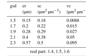
Table 1 summarizes the parameters of the PSDs that were used in the simulation studies. Additional explanations are given in Sect. 3.1.
Table 1.Input parameters of the particle size distributions used in the simulation studies. We used monomodal PSDs with mean radius 100 nm. We used PSDs normalized to one particle per cm3, gsd (σ) denotes the geometric standard deviation (mode width), er is the effective radius, sc is the surface area concentration, and vc the volume concentration.
gsd er sc vc
(µm) (µm2µm−3) (µm2µm−3)
1.5 0.15 0.18 0.0088
1.7 0.2 0.22 0.015
1.9 0.28 0.29 0.027
2.1 0.4 0.38 0.05
2.3 0.57 0.5 0.095
real part: 1.4, 1.5, 1.6
imaginary part: 0, 0.005, 0.01, 0.03, 0.05
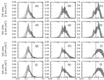
Figure 2 shows examples of PSDs retrieved with the TRO-POS/UH algorithm. The task of deriving the shape of the par-ticle size distribution is challenging as we are dealing with a small number of optical data, i.e. the information content of the set of optical data is low. However, during our develop-ment work we noticed that we can obtain some information on the particle size distribution too.
The panel shows the results for moderately absorbing aerosols, i.e. the imaginary part is 0.01i. The first row (a– c) shows the results for error-free data and the assumption that the real part can be derived to an uncertainty of 0.1. The second row (d–f) shows the results for error-free data and the ideal case that we can derive the real part to 0.05 accuracy. The rationale for using these uncertainties of 0.1 and 0.05 will be given in Sect. 3.1. The third row (g–i) shows the re-sults for a measurement error of 15 % and an uncertainty of 0.1 of the real part. The fourth row (j–l) shows the results for the measurement error of 15 % and an uncertainty of 0.05 of the real part.
0.00 0.01 0.02 0.03 0.04 0.05
(a)
0.00 0.05 0.10 0.15 0.20 0.25
(b)
0.0 0.2 0.4 0.6 0.8 1.0
(c)
0.00 0.01 0.02 0.03 0.04 0.05
(d)
0.00 0.05 0.10 0.15 0.20 0.25
(e)
0.0 0.2 0.4 0.6 0.8 1.0
(f)
0.00 0.01 0.02 0.03 0.04 0.05
(g)
0.00 0.05 0.10 0.15 0.20 0.25
(h)
0.0 0.2 0.4 0.6 0.8 1.0
(i)
0.01 0.1 1 10
0.00 0.01 0.02 0.03 0.04 0.05
µ (j)
µ 0.01 0.1 1 10
0.00 0.05 0.10 0.15 0.20 0.25
(k)
0.01 0.1 1 10
0.0 0.2 0.4 0.6 0.8 1.0
(l)
Vol. conc.
Vol. conc.
Vol. conc.
Vol. conc. [1 (cm m) ]
-1
µ
[1 (cm m) ]
-1
µ
[1 (cm m) ]
-1
µ
[1 (cm m) ]
-1
Radius [ m] Radius [ m]µ Radius [ m]µ
Figure 2.Examples of retrieved particle size distributions for the case of the geometric standard deviation of 2.1, real part of 1.5, imaginary part of 0.01iand for mean radius of(a, d, g, j)60 nm,(b, e, h, k)140 nm, and(c, f, i, l)300 nm. The true PSD is shown as red curve. The retrieved mean PSDs are shown as solid light blue lines and error bars (grey) in terms of 1σstandard deviation. The error bars are plotted on a dense grid and follow from the averaging of several hundred individual inversion solutions for each of the mean PSDs. The vertical lines are positioned at 500 nm particle radius. We define 500 nm particle radius as separation between fine-mode and coarse-mode particles. Row
(a–c)represents the results from using the constraint that the real part is known to 0.1 in the data inversion and that the optical data are error free. Row(d–f) shows the results for error-free data and that the real part is known to 0.05. Row(g–i)shows the results if the real part is known to 0.1 and that the optical data have an extreme error of 15 %. Row(j–l)shows the results if the real part is known to 0.05 and that the optical data have an extreme error of 15 %.
we average all individual PSDs, the mean solution is compa-rably close to the true PSD.
2.2 UP algorithm
2.2.1 Solving the Fredholm equations and description of the software
The Potsdam algorithm (UP) uses TSVD as a hybrid reg-ularization method and collocation with B splines Bj(r), j =1, . . ., n, of variable order d. The discretization tech-nique of the Fredholm integral Eq. (3) itself follows the same rules as the TROPOS/UH algorithm (see Eqs. 6, 7). For more details about the TSVD we refer to Engl et al. (1996), Hansen (2010), and Böckmann (2001). In contrast to the TROPOS/UH algorithm, the UP method uses the number nand the orderdof the B splines as the first two regulariza-tion parameters. The TROPOS/UH algorithm uses the fixed order 2, i.e. B splines with triangular shape. We found that if we use TSVD, the number and shape of the B splines has a large influence on the accuracy of the inverted PSD. Our
experience shows thatn=3, . . .,8 andd=3,4 are the most appropriate parameters.
It is a well-known fact (e.g. Hansen (2010)) that the dis-cretization dimension (number n of used B splines) has reg-ularization properties. The matrixAis decomposed uniquely into A=VTD U by orthonormal matrices U and V. D is a rectangular diagonal matrix. This matrix contains non-negative singular values that cluster to zero. Since small sin-gular values amplify the data noise (measurement errors) and generate oscillations in the solution, namely the PSD, it is necessary to truncate them. The truncation level of the sin-gular valuesk=0, . . .,min(5, n)−1 is the third regulariza-tion parameter of the hybrid method. Thus we obtain a triple (d, n, k)of parameters.
The linear equation systemAf =(VTD U)f =ghas to be solved for each parameter triple, e.g.n=3, . . . ,8, d=
3,4 andk=0, . . . ,min(5, n)−1; we note that matrix Ais derived in Eq. (6). The PSDf (r)is determined from a lin-ear combination of a particular set of B splines (number and order) asf (r)=Pn
constraint that is included in addition in the retrieval of the PSD is explained by Böckmann (2001).
The spline number n and order d are parameters that are not independent of each other. These two parameters are related to each other through the number of B-spline nodes. Our algorithm can use an equidistant or a equidistant node grid. For the latter option we employ a non-equidistant grid that uses the Chebyshev polynomial roots for these nodes. These nodes are transformed into the inter-val [rmin, rmax]to avoid frequently observed characteristics
(e.g. oscillations) of the PSD.
Figure 1 shows a screenshot of the developed software. The workflow of the software is split into a set-up, compu-tation, and evaluation step. The set-up step allows the user to specify input data, define the parameter space that will be searched, configure a simulation, and select retrieval meth-ods. The goal of this step is to create a job description that is fed into the computation step.
For the computation step, we have developed a parallel software that allows us either to cope with the vast parame-ter space or to enable us to carry out a more refined search for a solution. This part of the software is designed such that it runs separately from the interactive set-up and evaluation step. In this way it can be used for parallelized execution on a supercomputer or a computer cluster. A master process splits the work task into small units and delegates the calculations to any available worker process. Once a worker has com-pleted its task, it returns the results to the master. The current search algorithm allows for what we describe as embarrass-ingly parallel processing (i.e. it does not require any inter-action between the workers and therefore scales to a large number of workers (Osterloh et al., 2009).
The screenshot in Fig. 1 was taken from the result-evaluation step after completion of one of the inversion com-putations. We use the Qt cross-platform application frame-work. The Qt-based front-end allows the data operator to in-teractively explore the results and plot further details (right box) for selected coordinates (grid points) (left box).
It is obvious that including the wavelength- and size-independent complex refractive index grid, (Fig. 1; left box), the solution space of the algorithm is quite huge. It contains
|n|×|d|×|k|×|RPCRI|×|IPCRI|solutions in total. The term
| · |denotes the number of different values of the specific
pa-rameter. The solution space is restricted in the following way: for every specific refractive index the best triple(d, n, k)is picked in terms of least residual error. In contrast to the TRO-POS/UH algorithm that uses Eq. (7), we find this least resid-ual error from Eq. (3) and forward calculation. In the next step, the best triple at each grid point is used. The associ-ated least residual error is presented on a logarithmical colour scale which displays the error magnitude (Fig. 1). This visual representation is very convenient for the post-processing pro-cedure. At this point we are able to evaluate three different coloured refractive index grids with respect to three different mathematical norms: the Euclidian norm of the absolute and
of the relative error, and the maximum norm of the relative error.
As already mentioned in the introduction, a second regu-larization technique has been included in the software for the purpose of comparison. This regularization technique solves the linear equation systemAf =gin contrast to TSVD by using an iterative regularization method. Kirsche and Böck-mann (2006) and BöckBöck-mann and Kirsche (2006) developed a whole family of Páde iterations that are used to solve lin-ear equation systems by means of regularization. The well-known Landweber iteration is a member of this family (e.g. Hansen (2010)). We deal again with a triple of parameters (d, n, j ), where the third one is now the number of iteration stepsj. The number of iteration steps depends on the data noise levelε according to j = bε−1c. The termbε−1c de-notes the integer part of the real number 1/ε. Simulations have shown thatj= bε−1cis an appropriate choice. In case of an unknown noise levelε,j=30 is a good choice, e.g. for moderate absorption. To account for the non-negative restric-tion of the PSD we use a projected iterarestric-tion (Osterloh et al., 2011).
As noted above there is a strong connection between the distribution of the B-spline nodes and the quality of the re-constructed PSD. To take this connection into considera-tion, the Páde algorithm adapts the nodes according to cer-tain rules. Indeed, it is easy to see how the PSD is strongly smoothed out in areas in which only a few nodes exist. Strong slopes and curvatures of the PSD require many nodes in their vicinity for an accurate reconstruction. In order to account for this behaviour, the nodes automatically slide towards radius intervals that have larger weight in the PSD during the itera-tion process, in contrast to fixed non-equidistant Chebyshev nodes. For more details we refer to Osterloh et al. (2011). If we use either TSVD or Páde regularization, we obtain a log-arithmically coloured refractive index grid that indicates the error magnitude, as explained above (Figs. 1, 3).
Forward calculations provide us with backscatter and ex-tinction coefficients, which are subsequently used in the data inversion. Even in the noiseless case in which these input data are computed without explicitly considering measure-ment errors, we still obtain uncertainties because approxima-tion and rounding errors are added to the coefficients, i.e. the input data that are used in the inversion are not truly noise-less. Even those small errors can be harmful for an ill-posed inversion problem.
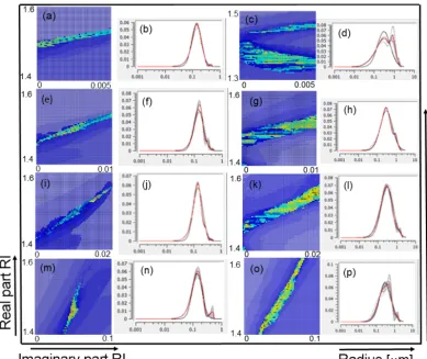
Fig-Figure 3.Examples of colour-coded refractive index grids and PSDs for noiseless input data. The rows correspond to different imaginary parts of the CRI: 0, 0.005, 0.01 and 0.05. The first two columns contain fine-mode particles with gsdσ=1.5 and real part 1.5. We used equidistant B-spline nodes. The third and fourth columns correspond to intermediate-mode particles with gsdσ=2.1, real part of CRI 1.5 and non-equidistant B-spline nodes, except(c),(d)with real part 1.4 and equidistant nodes. The mean PSD (the solution) is drawn as red single line.
ure 3 for the most part shows the maximum norm except for (c), (g), and (i) where the Euclidean norm of the absolute error is shown.
The selection procedure is easier for fine-mode particles (Fig. 3, first column) than for fine-coarse- and coarse-mode particles (not shown here) since the best CRIs are located along a very narrow diagonal, in particular with regard to real part 1.5 as shown in Fig. 3a, e, i, and m. We assume that this diagonal structure indicates a lack of information, which keeps us from determining the refractive index uniquely. However, we will give an estimation of the CRI by using the mean of approximately 10 to 20 best values; details are given below.
For the real part 1.4 the diagonal structure more or less dis-appears for fine-coarse- (Fig. 3c) and coarse-mode particles (not shown here) except for strongly light-absorbing parti-cles of imaginary part 0.05i. We observe a similar behaviour for the same particle types if the real part is 1.6 with non-absorbing or weakly non-absorbing particles (imaginary part 0i and 0.005i), not shown here. Columns 1 and 3 of Fig. 3 show
that the selection procedure of the CRI becomes easier with increasing imaginary part. We note that we did not use larger coarse-mode particles, e.g. the case ofσ =2.5, in our simu-lation study because of the ill-posedness from a mathemati-cal point of view, i.e. the smoothness of the kernel function in Eq. (1). Our investigations show that the Potsdam algorithm should not be used for radii larger than 5–7 µm depending on the refractive index (rule of thumb) (see Osterloh et al. (2013) and Samaras et al. (2015)).
2.2.2 Identification of the solution space for UP algorithm
In this section we explain the selection procedure of CRI and PSD. The main selection criteria are based on our knowledge of working with simulated and experimental data for the case of a grid mesh of 30×30 to 60×60 grid points (see Figs. 1 and 3).
selec-tion results in a good representaselec-tion of the PSD (Fig. 3a, e, i, m). Isolated grid points which are not located in a cluster inside the diagonal region or in a cluster inside an arbitrar-ily shaped region (see Fig. 3c) should be removed even in the case that a good mathematical approximation of the PSD exists. But usually the approximation of the PSD that results from isolated grid points is not very good. Physically mean-ingful PSDs appear in clusters.
Second, if grid points form a thin vertical or horizontal line and additionally provide a bad approximation of the solution, i.e. of the PSD, all data points along the vertical or horizon-tal line should be removed. Grid points that appear isolated at the end of a diagonal or an arbitrarily shaped region (we denote them as boundary points) may be removed.
Third, as a rule of thumb one should select at least 10 and at most 20 grid points. If meaningful, one can use accumu-lative two or three mathematical norm grids of the refractive index (as previously explained). If more than one cluster ex-ists and if these clusters have the same number of solutions it is difficult to decide which cluster should be preferred. Changing the mathematical norm grid may help in the de-cision making. For more details see Samaras et al. (2015).
Finally, for fine-mode particles (σ=1.5,1.7, i.e. narrow mono-lognormal PSD) we suggest using an equidistant B-spline node grid. However, our experience shows that better results can be achieved for coarse-mode particles (σ=2.3, expanded mono-lognormal PSD) with a non-equidistant grid of left-hand Chebyshev nodes.
Furthermore, the use of the Páde iteration as regulariza-tion method often leads to very good results with respect to the pattern of the obtained refractive index grid. There-fore, the manually controlled selection process of the CRI, as described above, often can be performed more easily with Páde iteration than with TSVD regularization. This is es-pecially true for the PSD examples σ=1.5,1.7,1.9 (fine-and intermediate-mode particles), independent of the real (fine-and imaginary part of the CRI. In all cases, the selection process of the CRI grid points that are associated with the best PSD solutions is very easy to do since the best solutions in most CRI grids form distinctive diagonals (not shown here).
In general grid points are not isolated, i.e. all points are located in clusters. If a diagonal structure is absent, we know from experience that meaningful solutions can be identified in arbitrarily shaped clusters too (Samaras et al., 2015). Only broader modes,σ =2.1,2.3, seem to be occasionally prob-lematic in terms of seeking a solution cluster, which could lead to oscillatory PSDs. Therefore, the use of the Páde iter-ation is a huge improvement. Nevertheless, it should be men-tioned that the retrieved mean PSD is less accurate in the case of small particle radii compared to the PSD obtained with TSVD. Therefore, the Páde iteration was not used in this simulation study. It is an ongoing work to combine the methods in an appropriate way to make use of the different advantages associated with both methods.
2.2.3 Particle size distribution: examples
The UP algorithm was tested with the same examples (Ta-ble 1) as the TROPOS/UH algorithm. The selection of the best CRI grid points, i.e. the mean CRI, is always strongly connected with the corresponding PSD, i.e. we look for sim-ilar shapes of the PSD. The retrieved mean PSD solution, Figs. 3, 4 (solid red line), is the average of 10 to 20 PSDs (solid grey lines) corresponding to the selected 10 to 20 CRI grid points as described in the last section (true PSD: solid black line).
Figure 3 shows eight examples of retrieved PSDs for the case of noiseless data. In that case it is possible to retrieve the monomodal lognormal shape of the input PSD very well with regard to accuracy and precision in almost all exam-ples, in particular peak height and location match accurately (Fig. 3). We note (not shown here) that a second peak very of-ten occurs for coarse-mode particles (gsdσ=2.3), although this second peak is very small in most cases. The excep-tions are weakly absorbing (0.005i, 0.01i) particles with real parts around 1.4. In that case the PSD is monomodal. For non-absorbing particles or strongly light-absorbing particles (0.05i) with real part 1.4, the second peak also occurs for gsd σ=2.1 (Fig. 3d) and gsdσ=1.9 (not shown here).
In summary, the retrieval of the PSD in the case of noise-less data is excellent with regard to retrieval accuracy and re-trieval precision. Only for almost all real and imaginary parts in the coarse-mode case and for fine-coarse-mode cases with real parts around 1.4 and imaginary parts of 0iand 0.05i re-spectively, the retrieved PSDs show a small second peak. But this second peak probably is only a mathematical feature (os-cillation) which cannot be smoothed out during the regular-ization process. The reason for this second peak is probably the larger ill-posedness of the underlying mathematical prob-lem.
Figure 4 shows 16 examples of retrieved PSDs for the case of noisy data (random Gaussian noise of 15 %, 10 runs per example). Most of the results are good, in particular for gsd 1.7 and 1.9 where the accuracy of the results is very good (Fig. 4, second and third column). In the case of noisy in-put data, oscillations of the PSDs that describe coarse-mode particles (gsdσ=2.3) occur. These PSDs show a second or even a third peak for all CRIs considered in this study. How-ever, the retrieval accuracy is good (except for strongly light-absorbing particles with 0.05i (Fig. 4p). In contrast, retrieval precision is not that good. Additionally, all PSDs coupled with real part 1.4 and gsd 1.7–2.1 show more or less a sec-ond peak for all imaginary parts (not shown here).
The retrieved PSDs of fine-mode particles with gsdσ=
Figure 4.Examples of PSDs for input data with 15 % noise: the rows correspond to different imaginary parts of the CRI: 0, 0.005, 0.01, and 0.05. The columns correspond to gsd: 1.5, 1.7, 1.9, 2.3. The real part of CRI is 1.5. The mean PSD, i.e. the solution, is shown as a solid red line.
independent of the value of the imaginary part (not shown here).
For the combination of real parts 1.5 and 1.6 and σ=
1.7,1.9 the retrieved PSDs (red solid lines) are monomodal. The peak height and its location show excellent overlap to the peak height and location of the initial distribution (black solid lines) for all imaginary parts. Examples are shown in Fig. 4, second and third column, for real part 1.5. The accu-racy and precision is very high even in the case of noisy data. In contrast, forσ=2.1 (not shown here) the peak height is often a little bit overestimated, but the peak location is only slightly shifted to the left or right.
In summary, if 15 % noise is added to the input data, the PSD can still be retrieved quite well for fine-coarse-mode particles in the case of real parts 1.5 and 1.6 in combination with all imaginary parts.
3 Simulation results and discussion
3.1 Generation of optical data for retrieving microphysical parameters
Table 1 shows the parameters of the particle size distributions (effective radius and geometric standard deviation) and the CRIs that were used for the computations of the optical input data. We used five different effective radii.
Effective radii of 0.15 and 0.2 µm are in the size range of the fine-mode fraction of particle size distributions. Effective radii of 0.28 and 0.4 µm describe particle size distributions that have a significant share of particles in the coarse-mode fraction and the fine-mode fraction. An effective radius of 0.57 µm describes a size distribution for which most of the particles are in the coarse-mode fraction of the particle size distribution.
With regard to the complex refractive indices we tested three real parts, i.e. 1.4, 1.5, and 1.6. In our opinion these values cover a realistic range of real parts that can be ex-pected for atmospheric particles. Values of around 1.4 de-scribe highly refractory particles. Sea salt belongs to this class of particles. The value of 1.5 can be used to describe industrial pollutants, for example sulfuric acid. Soot has a high real part of 1.8, but it is usually not found in pure form. Thus, if soot mixes with other aerosol components the real part reduces. We estimate that 1.6 is a representative value for pollution particles, for example biomass burning particles that contain some amount of black carbon.
The imaginary part varies over several orders of magni-tude. Our goal in our software development is that we can find the correct value at least to within±50 %.
An accuracy of approximately±0.03 for single-scattering albedo is often assumed as a basic requirement in order to test the sensitivity of light-absorbing aerosols in climate change studies. This accuracy, however, cannot be expressed in terms of a single number of the accuracy of the imaginary part. The reason for it is that the particle size distribution also influ-ences the value of the SSA. A small change of the imaginary part may have a significant impact on the SSA if the particles are in a specific radius range. A small change of the imag-inary part may not have a significant impact on the SSA if the particles are in another part of the radius range of atmo-spheric particles. We currently cannot quantify by how much the SSA changes if particle size and/or complex refractive in-dex change by a certain amount. Detailed simulation studies (e.g. forward Mie-scattering computations) for a wide range of scenarios of PSDs and CRIs would be required. This work goes beyond the scope of the current study.
In the first step we used the UP algorithm to test if we are able to derive the imaginary part to within±0.005 in ab-solute values. We used the TROPOS/UH algorithm to find out the accuracy of all other retrieved microphysical param-eters, assuming that the real part can be derived to ±0.05 or ±0.1 accuracy. We investigated if this constraint on the real part allows for retrieving the imaginary part to±0.005. This accuracy of ±0.005 may in fact not be achievable, at least not for arbitrary particle scenarios, but it would signifi-cantly increase our chances to retrieve highly accurate values of single-scattering albedo.
We had to restrict our simulations to a few imaginary parts because the inversion algorithms are manually oper-ated and the data analysis is time consuming. We selected a few imaginary parts that were meant to give us a reasonable
overview on the retrieval performance if particles are non-absorbing (imaginary part=0i) and if particles are highly light-absorbing (imaginary part=0.05i).
One point that must be considered in these simulations is the fact that, with regard to experimental conditions, we likely will not find all possible combinations of the particle size parameters (effective radius, real, and imaginary part of the complex refractive index) listed in Table 1. The reason why we believe that this will not happen can be seen from the following Table 2.
Table 2 shows the minimum and maximum values of the extinction-related and backscatter-related Ångström expo-nents that follow from the combinations of the five effective radii and the CRIs listed in Table 1. The other three values (five in total) for each of the Ångström exponents fall within these minimum and maximum values. We also show the indi-vidual values of the lidar ratios, and the ratio of the two lidar ratios (at 355 and 532 nm) that we obtain from all the com-binations of the real and imaginary parts for each effective radius tested in this sensitivity study.
The extinction-related Ångström exponents largely cover the range of values we found from measurements of extinc-tion coefficients at 355 and 532 nm. We regularly measure extinction-related Ångström exponents of 1–2 in regions that are affected by anthropogenic pollution. Maximum values that have been measured are as high as 2.5, but we did not test this scenario in our study.
Values below 1 describe large particles in the coarse-mode fraction of particle size distributions. The most likely can-didate of an aerosol type with extinction-related Ångström exponents below 1 is mineral dust. However, we cannot sim-ulate with reasonable confidence optical data that describe mineral dust particles. Until now we could not identify a light-scattering model that would allow us to model trust-worthy values of particle backscatter coefficients, i.e. scat-tering at 180◦. However, in the past we measured extinction-related Ångström exponents of 0.5–1. Such values are extinction-related to aged biomass burning aerosols (Müller et al., 2005). In a few instances, extinction-related Ångström exponents of aged biomass burning aerosols were less than 0.5.
We also considered the case of extinction-related Ångström exponents around 0. Again, this scenario most likely occurs if large mineral dust particles are present. How-ever, large sea-salt particles may also show extinction-related Ångström exponents of around 0 and for that reason we sim-ulated such cases as well. We point out that it is not unlikely to find extinction-related Ångström exponents slightly less than 0, as shown in Table 2. It is unclear if negative values can be resolved by Raman lidar measurements in view of re-alistic measurement errors of 10–20 %.
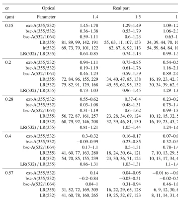
Table 2.Input parameters of the size distributions used in the simulation studies. We used monomodal PSDs with mean radius 100 nm and 5 different geometric standard deviations. We used PSDs normalized to one particle per cm3. The parameter ext-A(355/532) denotes the extinction-related Ångström exponent for the wavelength pair 355/532 nm, while bsc-A(355/532) and bsc-A(532/1064) denote the backscatter-related Ångström exponents for the wavelength pairs 355/532 nm and 532/1064 nm respectively. LR(355) and LR(532) denote the lidar ratios at 355 and 532 nm respectively. LR(532)/LR(355) denotes the colour ratio of the lidar ratios at 355 to 532 nm. We use five different imaginary parts for each pair of effective radius and real part. For that reason we obtain five different lidar ratios for each of these pairs. In the case of the Ångström exponents, we show the range from minimum to maximum value instead of the five individual values. That range of values arise from the choice of different input parameters used for the particle size distributions.
er Optical Real part
(µm) Parameter 1.4 1.5 1.6
0.15 ext-A(355/532) 1.45–1.78 1.29–1.49 1.09–1.23
bsc-A(355/532) 0.36–1.38 0.53–1.79 1.06–2.37
bsc-A(532/1064) 0.59–1.11 0.6–1.23 0.63–1.4
LR(355) 81, 89, 99, 142, 191 55, 63, 11, 107, 153 34, 39, 44, 70, 106 lr(532) 69, 73, 79, 101, 122 62, 67, 8, 92, 113 54, 59, 64, 84, 105
LR(532)/LR(355) 0.64–0.85 0.74–1.13 0.99–1.59
0.2 ext-A(355/532) 0.94–1.11 0.73–0.85 0.54–0.59
bsc-A(355/532) 0.19–1.19 0.61–1.76 1.16–2.12
bsc-A(532/1064) 0.46–1.23 0.59–1.59 0.89–2.03
LR(355) 72, 84, 96, 155, 229 34, 40, 47, 85, 138 16, 19, 23, 42, 72 LR(532) 75, 82, 91, 129, 168 49, 55, 62, 95, 132 30, 34, 39, 62, 93
LR(532)/LR(355) 0.73–1.03 0.96–1.45 1.29–1.86
0.28 ext-A(355/532) 0.55–0.62 0.37–0.4 0.23–0.24
bsc-A(355/532) 0.03–1.08 0.48–1.31 0.75–1.47
bsc-A(532/1064) 0.31–1.19 0.6–1.62 0.99–1.95
LR(355) 56, 72, 87, 161, 257 23, 28, 34, 69, 124 10, 12, 15, 32, 59 LR(532) 68, 79, 92, 146, 208 32, 39, 46, 81, 130 16, 19, 23, 43, 73
LR(532)/LR(355) 0.81–1.21 1.05–1.44 1.24–1.64
0.4 ext-A(355/532) 0.3–0.32 0.16–0.17 0.07–0.08
bsc-A(355/532) −0.09–0.99 0.23–0.85 0.32–0.94
bsc-A(532/1064) 0.17–1.1 0.5–1.31 0.78–1.48
LR(355) 41, 60, 77, 163, 280 18, 24, 30, 64, 121 7, 10, 13, 29, 57 LR(532) 54, 70, 85, 155, 239 23, 30, 36, 71, 124 10, 13, 17, 34, 63
LR(532)/LR(355) 0.86–1.31 1.03–1.31 1.1–1.42
0.57 ext-A(355/532) 0.14 0.04–0.05 −0.01 to−0.02
bsc-A(355/532) −0.2–0.84 −0.03–0.51 −0.02–0.56
bsc-A(532/1064) 0.04–1 0.31–0.94 0.46–1.04
LR(355) 31, 52, 72, 169, 305 16, 22, 29, 65, 128 6, 9, 12, 30, 60 LR(532) 41, 60, 78, 160, 265 19, 25, 32, 67, 123 8, 11, 14, 31, 60
LR(532)/LR(355) 0.87–1.33 0.97–1.21 1–1.27
There remains the question of whether it is justified to simulate scenarios in which lidar ratios considerably exceed 100 sr or drop below 20 sr. We believe that we should con-sider such extreme outliers in at least a few studies for two reasons. First, we can test the robustness of our algorithms for such extreme cases. The second point is that the under-lying microphysical properties do not seem to be completely out of range of numbers we can expect for atmospheric ticles. It is simply the combination of specific values of par-ticle size distribution and CRI that creates these outliers of lidar ratios.
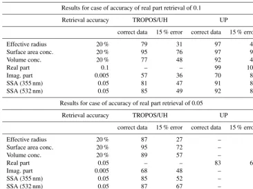
Table 3.Percentage of simulation cases that result in given retrieval accuracy.
Results for case of accuracy of real part retrieval of 0.1
Retrieval accuracy TROPOS/UH UP
correct data 15 % error correct data 15 % error
Effective radius 20 % 79 31 97 43
Surface area conc. 20 % 95 76 97 99
Volume conc. 20 % 77 48 92 47
Real part 0.1 – – 99 100
Imag. part 0.005 57 36 70 82
SSA (355 nm) 0.05 81 47 91 88
SSA (532 nm) 0.05 85 49 92 88
Results for case of accuracy of real part retrieval of 0.05
Retrieval accuracy TROPOS/UH UP
correct data 15 % error correct data 15 % error
Effective radius 20 % 87 27 – –
Surface area conc. 20 % 95 72 – –
Volume conc. 20 % 89 57 – –
Real part 0.05 – – 83 64
Imag. part 0.005 68 48 – –
SSA (355 nm) 0.05 85 52 – –
SSA (532 nm) 0.05 87 67 – –
(2014)). We made use of this possibility in this study. We explicitly did not attempt to further optimize our inversion results by selecting a subset of best possible solutions in the sense of manually selecting solutions from the solution space that follows from constraining the real part to either 0.05 or 0.1. We obtain a family of individual solutions for which the real part is within either 0.1 or 0.05 deviation from the true value. We average this family of solutions and thus obtain mean value and uncertainty, which in this study will be ex-pressed in terms of accuracy (systematic error or bias) and precision (statistical error or noise).
We also tested our algorithm under the assumption of com-parably unfavourable measurement error scenarios. We dis-torted each optical data point by its maximum value of ei-ther 5, 10, or 15 %. In that regard, errors of 15 % represent the worst case scenario in this study. We did this distortion without considering the possibility that data points may be correlated to each other and thus error bars may also not be independent of each other. We assume that the inversion of such ”extremely” distorted backscatter and extinction spectra would result in microphysical parameters that also deviate to a maximum value from the correct values. This assumption of course has the flaw that the inversion is a non-linear prob-lem. That means an extreme distortion of optical input data may not necessarily need to lead to a maximum deviation of the retrieved microphysical parameters from their true val-ues. However, we believe that we will learn more about this
type of error analysis in this first attempt and that we can refine it in future studies.
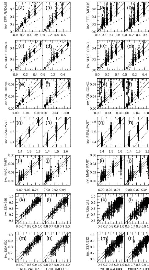
3.2.1 Results for error cases 0 and 15 %
Figure 5 shows a summary of the retrieval performance of the TROPOS/UH algorithm with regard to effective radius, number, surface area, and volume concentration, and the real and imaginary part. The left panel shows the results of simu-lations carried out for error-free data. The right panel shows the extreme error estimation of the retrieval results.
According to Chemyakin et al. (2014), the real part of the CRI of the optical data we used in this study can be retrieved to an accuracy of approximately 0.1 with 2σ confidence for the case of noiseless optical data (Table 3 in Chemyakin et al. (2014)). We made use of this result in our simulations as we are mainly interested in finding out about the performance of the algorithm under favourable conditions of the input pa-rameters. For example, we are looking for ways that allow us to constrain the search space of the refractive index grid, as the retrieval of the refractive index poses the greatest chal-lenge in our work.
0 . 0 0 0 . 0 5 0 . 0
0 . 1 0 . 2 0 . 3 0 . 4 0 . 5 0 . 6 0 . 7
( a )
E F F . R A D IU S µ m ]
0 . 0 0 0 . 0 5
( b )
0 . 0 0 0 . 0 5
( c )
0 . 0 0 0 . 0 5 0 . 0
0 . 1 0 . 2 0 . 3 0 . 4 0 . 5 0 . 6
( d )
S U R F . C O N C . [ µ m 2 c m 3 ]
0 . 0 0 0 . 0 5
( e )
0 . 0 0 0 . 0 5
( f )
0 . 0 0 0 . 0 5 0 . 0 0
0 . 0 3 0 . 0 6 0 . 0 9 0 . 1 2 0 . 1 5
V O L . C O N C . [ µ m
3 cm 3 ]
( g )
0 . 0 0 0 . 0 5
( h )
0 . 0 0 0 . 0 5
( i )
0 . 0 0 0 . 0 5 1 . 3
1 . 4 1 . 5 1 . 6 1 . 7
R E A L P A R
T
( j )
0 . 0 0 0 . 0 5
( k )
0 . 0 0 0 . 0 5
( l )
0 . 0 0 0 . 0 5 0 . 0 0
0 . 0 2 0 . 0 4 0 . 0 6 0 . 0 8
IM A G . P A R
T
( m )
0 . 0 0 0 . 0 5
( n )
0 . 0 0 0 . 0 5
( o )
0 . 0 0 0 . 0 5 0 . 6
0 . 7 0 . 8 0 . 9 1 . 0
( p )
S S A 3 5 5
0 . 0 0 0 . 0 5
( q )
0 . 0 0 0 . 0 5
( r )
0 . 0 0 0 . 0 5 0 . 6
0 . 7 0 . 8 0 . 9 1 . 0
S S A 5 3 2
( s )
I M A G . P A R T , R E A L P A R T = 1 . 4
0 . 0 0 0 . 0 5
( t )
I M A G . P A R T , R E A L P A R T = 1 . 5
0 . 0 0 0 . 0 5
( u )
I M A G . P A R T , R E A L P A R T = 1 . 6
0 . 0 0 0 . 0 5 0 . 0
0 . 1 0 . 2 0 . 3 0 . 4 0 . 5 0 . 6 0 . 7 0 . 8 0 . 9 1 . 0
( a )
E F F . R A D IU S [ µ m ]
0 . 0 0 0 . 0 5
( b )
0 . 0 0 0 . 0 5
( c )
0 . 0 0 0 . 0 5 0 . 0
0 . 1 0 . 2 0 . 3 0 . 4 0 . 5 0 . 6
( d )
S U R F . C O N C . [ µ m 2 c m 3 ]
0 . 0 0 0 . 0 5
( e )
0 . 0 0 0 . 0 5
( f )
0 . 0 0 0 . 0 5 0 . 0 0
0 . 0 3 0 . 0 6 0 . 0 9 0 . 1 2 0 . 1 5
V O L . C O N C . [ µ m
3 cm 3 ]
( g )
0 . 0 0 0 . 0 5
( h )
0 . 0 0 0 . 0 5
( i )
0 . 0 0 0 . 0 5 1 . 3
1 . 4 1 . 5 1 . 6 1 . 7
R E A L P A R
T
( j )
0 . 0 0 0 . 0 5
( k )
0 . 0 0 0 . 0 5
( l )
0 . 0 0 0 . 0 5 0 . 0 0
0 . 0 2 0 . 0 4 0 . 0 6 0 . 0 8
IM A G . P A R
T
( m )
0 . 0 0 0 . 0 5
( n )
0 . 0 0 0 . 0 5
( o )
0 . 0 0 0 . 0 5 0 . 6
0 . 7 0 . 8 0 . 9 1 . 0
( p )
S S A 3 5 5
0 . 0 0 0 . 0 5
( q )
0 . 0 0 0 . 0 5
( r )
0 . 0 0 0 . 0 5 0 . 6
0 . 7 0 . 8 0 . 9 1 . 0
S S A 5 3 2
( s )
I M A G . P A R T , R E A L P A R T = 1 . 4
0 . 0 0 0 . 0 5
( t )
I M A G . P A R T , R E A L P A R T = 1 . 5
0 . 0 0 0 . 0 5
( u )
I M A G . P A R T , R E A L P A R T = 1 . 6
Figure 5.Left panels: TROPOS/UH algorithm retrieval results for(a–c)effective radius,(d–f)surface area concentration,(g–i)volume concentration,(j–l)real part, and(m–o)imaginary part of the complex refractive index, and single-scattering albedo at(p–r)355 nm and
(s–u)532 nm. The left segment shows the results for real part 1.4, the centre segment shows the results for real part 1.5, and the right segment shows the results for real part 1.6. Our inversion results are obtained with an upper threshold of the real part of 0.1 (boxes) and a threshold of 0.05 accuracy (circles). The error bars denote 1 standard deviation. Right panels: results of our extreme error analysis for the case of 15 % measurement error. Upward-pointing triangles refer to results for which the real part was constrained to 0.05. Downward-pointing triangles refer to inversion results for which the real part was constrained to 0.1. Meaning of the other symbols is the same as in the left panel.
coarse mode, the performance on average still is acceptable (in view of the uncertainty bars) although we find outliers for particles with real parts of 1.4.
Surface area concentration on average shows exception-ally high accuracy. The precision (the uncertainty bars re-flect the statistical noise in terms of 1 standard deviation) is high compared to the error bars we obtain for effective radius and volume concentration. We find one outlier (see Fig. 5e) which cannot be explained at the moment.
Volume concentration in general shows the same features as effective radius, i.e. the retrieval accuracy is generally good for particles in the fine-mode fraction. We find some outliers for the intermediate cases and the coarse-mode case, mainly for real parts of 1.4.
The real parts follow from the application of the method-ology suggested by Chemyakin et al. (2014) (see Table 3 in Chemyakin et al. (2014)). If the real part is known, we can derive the imaginary part too, as the solutions for the real and imaginary part are correlated. An example of what this cor-relation looks like is shown for the UP algorithm in Fig. 1. Similar behaviour has also been found for the TROPOS/UH algorithm (see for example Fig. 3 in Müller et al. (2001b)).
The imaginary part can be found within±50 % uncertainty if imaginary parts are 0.01 or larger. This result has already been found in previous studies, e.g. Müller et al. (1999b). We know that we cannot derive the exact value if the imag-inary part is 0i. The inversion results for each data product are always the mean of several results. Thus, even if we as-sume that the correct optical data are used in the inversion, i.e. no error bars are considered, we end up with an overes-timation of the imaginary part. The reason for this situation is that we carry out the inversion for a grid of complex re-fractive indices. In general we will find acceptable inversion results even for cases in which the imaginary part is not 0i (Ansmann and Müller, 2005; Müller et al., 1999b). If we av-erage these individual values, we naturally obtain a bias to-ward mean values larger than 0i.
The noteworthy point and a new result compared over pre-vious studies is that our simulations give us an impression of the likely value of the overestimation of the imaginary part. If the true imaginary part is less than 0.01 we may overestimate the imaginary part by 0.005ion average. We hope that we can reduce this overestimation in future. One option could be that we refine our search grid of the imaginary part which is cur-rently set to 0.003i. That means the next nearest value to 0i that can be found with our algorithm is 0.003i. We assume
that this stepsize is likely to be one reason for the overesti-mation of the mean imaginary part (in the retrieval), which in turn leads to an underestimation of the single-scattering albedo for low light-absorbing aerosols particles.
Figure 5 also shows results if we assume that we could re-trieve the real part to an accuracy of 0.05 (open circles). In that case we again make use of the results published by Che-myakin et al. (2014), who show that an uncertainty of 0.05 is possible with 1-σ confidence if the arrange and average algorithm is applied.
The microphysical properties do not differ significantly from the results if the real part is retrieved to 0.1 accuracy and if we take account of the overall uncertainties of our in-version results. That is, any attempt to further improve the real part retrieval may not necessarily result in significant improvement of other data products and we consider this an important outcome of our study.
With regard to single-scattering albedo, Fig. 5 shows the results for each case separately, i.e. for each value of the true imaginary part we show five different results corresponding to the five different particle size distributions that we tested in the simulations. Thus, we show in total 25 different re-sults for each real part. The true value of single-scattering albedo in each column (corresponding to a specific value of the imaginary part and one of five possible effective radii) is shown by a thick horizontal coloured line. Each of these coloured horizontal lines can be linked to one symbol of the same colour. The symbol with that same colour represents the inversion result (mean value) of the underlying optical data set.
The retrieved single-scattering albedo on average can be derived to within±0.05 regardless of whether the real part is known to within 0.05 or 0.1. If single-scattering albedo is larger than 0.9, the inversion results become worse and tend to underestimate the true single-scattering albedo. If the true single-scattering albedo is 1, the retrieved value is around 0.95.