www.nonlin-processes-geophys.net/17/221/2010/ © Author(s) 2010. This work is distributed under the Creative Commons Attribution 3.0 License.
Nonlinear Processes
in Geophysics
The effect of volatile bubble growth rate on the periodic dynamics of
shallow volcanic systems
I. L’Heureux
Ottawa-Carleton Institute of Physics and Department of Physics, University of Ottawa, 150 Louis Pasteur, Ottawa, Ontario K1N6N5, Canada
Received: 26 January 2010 – Revised: 19 March 2010 – Accepted: 2 April 2010 – Published: 20 April 2010
Abstract. Many volcanic eruptions exhibit periodic
behav-ior. For instance, periodic ground inflations and deflations in proximity to a volcano are the consequences of periodic overpressure variations in the magma conduit and periodic magma flow rate. The period varies from a few hours to many years, depending on the volcano parameters. On the other hand, volatile components exsolve from an ascend-ing magma by formascend-ing bubbles. The strong dependence of the melt viscosity with the volatile concentration generates a positive feedback on the magma flow. We consider here the effect of the growth of volatile bubbles on the dynamics of a magmatic flow in a shallow volcanic system. Various expres-sions for the bubble growth rate are treated, thus generalizing previous work. In particular, a growth rate law derived from a recent many-bubble theory is considered. It is seen that, for a range of flow rate values at the base of the magma con-duit, the system undergoes a Hopf bifurcation. Periodic so-lutions compatible with the observations are generated. This work shows that measurements of volcanic activity have the potential to test various bubble growth models in magmatic systems.
1 Introduction
Volcanic eruptions are the consequences of a succession of complex processes acting over a wide range of timescales and understanding their dynamics is an important, but chal-lenging task. One example of intriguing volcanic eruptions dynamics consists in the occurrence of an oscillatory behav-ior. For instance, tilt meters installed on the crater of the Soufri`ere volcano (Montserrat Island) in 1996 and 1997 de-tected periodic ground inflations that correlated with periodic
Correspondence to: I. L’Heureux ([email protected])
seismic activity and periodic magma flow activity (Voight et al., 1998, 1999; Wylie et al., 1999). The period was of the order of 10–20 h. Other volcanic systems also exhibit cyclic episodes. Examples are found in Mount St. Helens (Wash-ington State, USA) between 1980 and 1986 (with an aver-age period of 74 days or 230 days, depending on the cycle) (Barmin et al., 2002), Santiaguito (Guatemala) from 1922 to the present (with an average period of 10.7 years) (Har-ris et al., 2003), Mount Unzen (Japan), Karymsky (Russia) and Merapi (Java) (Nakada et al., 1999; Ozerov et al., 2003; Voight et al., 2000).
On the other hand, various volatile species are commonly found in magmatic systems (mainly H2O, CO2 and sulfide species) and volatile bubble dynamics is an important con-tributing factor to the understanding of volcanic eruptions (Sparks, 1978; Bottinga and Javoy, 1990; De Vivo et al., 2005; Behrens and Gaillard, 2006; Proussevitch and Saha-gian, 1996, 1998). The object of this contribution is to ex-amine in details one simple nonlinear dynamical model in which an oscillatory behavior due to the growth of volatile bubbles occurs in a shallow volcanic system; the effects of various bubble growth rate laws are also investigated. The treatment is limited here to the typically dominant volatile species, water (De Vivo et al., 2005; Behrens and Gaillard, 2006).
Similar models are available in the literature. In Wylie et al. (1999) (thereafter referred to as WVW), the authors pre-sented a constant temperature model that is mostly applicable to shallow magmatic systems (such as Montserrat). In that model, the magma flow dynamics is coupled to changes in melt viscosity induced by variations in the dissolved volatile content (specifically water). In turn, through the forma-tion and growth of bubbles, volatile exsoluforma-tion controls the volatile concentration dynamics.
Macedonio (2002), a model is presented in which tempera-ture variations (rather than volatile content) induce changes in the melt viscosity, that feedback, in turn, on flow dy-namics. No dynamics are presented by these authors, but the possibility of a bursting effect (whereby the flow rate changes abruptly back and forth between two values) is de-scribed. Mourtada-Bonnefoi et al. (1999) presents a com-partment model in which crystal magma content and tem-perature are coupled through two ordinary differential equa-tions. Again, bubble bursting effects are described. How-ever, the model ignores transport processes. In Barmin et al. (2002) and Melnik and Sparks (1999, 2005), a more de-tailed transport model is described that takes into account the viscosity changes induced by variations in temperature and volatile content in a volcanic conduit of circular cross sec-tion. A crystal growth factor is also included in that model as the magma crystal content affects the permeability of the system and the flow dynamics. This model was further gen-eralized (Costa et al., 2007) to the situation where the lower part of the conduit has an elliptical cross section.
Other mechanisms that do not involve directly the pres-ence of volatile have been proposed to explain oscillatory eruptive behaviors. Ozerov et al. (2003) considered the magma as a visco-elastic fluid that undergoes stick-slip tran-sitions in a boundary layer adjacent to the conduit walls. They showed that an oscillatory behavior with short periods (seconds to minutes) may ensue.
In this paper, we generalize the WVW model in four ways: 1. In that model, it was assumed that the volatile concen-tration field adjusts quickly to its steady state value. Strictly speaking, this is valid only in the limit where the magma pressure relaxes very slowly in response to changes in magma flow rate. This is not true in general and we will not make this assumption here.
2. WVW introduced an approximation to simplify the mathematical treatment of their model: it was assumed that the integral of the viscosity has the same functional dependence as the integral of the volatile concentration field. As the relation between viscosity and volatile con-centration is not linear, this is not a correct assumption in general. We do not use this simplification here. 3. WVW uses a simple linear bubble growth law without
taking into account the degree of supersaturation. Here, we consider also more realistic bubble growth laws: the single bubble growth rate law in the diffusion-limit case (Navon and Lyakhovsky, 1998) and a recently published (L’Heureux, 2007) many-bubble growth law that takes into account (in the mean field sense) the collective ef-fect of the other bubbles on the growth of a given bub-ble.
4. Although a linear stability is presented by Nakanishi and Koyaguchi (2008) for the original Barmin et al.’s
model (2002), no detailed linear stability analysis is available for the WVW model, generalized to an arbi-trary bubble growth rate law. Such an analysis and a dynamical phase diagram in parameter space are pre-sented here.
The theory presented here is applicable to shallow magmatic systems (such as Montserrat) as it considers only the effect of volatile content on the melt viscosity and neglects tem-perature changes during the magma short ascent. Indeed, the time scale associated with conducting cooling of a shal-low ascending magma via heat exchange through the walls can be estimated from the magma thermal diffusivity (about 10−6m2/s, Costa and Macedonio, 2002) and the conduit lat-eral dimension (about 10 m); its value is very large compared to the relevant period of the oscillations (Voight et al., 1999). Over the time scales of interest here, we can thus neglect the cooling effect.
For simplicity, we also neglect the viscosity change due to increase in the magma crystal content. Previous models (Melnik and Sparks, 2005; Barmin et al., 2002) have param-eterized the viscosity dependence on crystal volume fraction in the following way: for a crystal volume fraction smaller than a critical value of about 0.7, the viscosity is basically constant; otherwise it increases rapidly with the crystal vol-ume fraction. For simplicity, we assvol-ume here that the crys-tal volume fraction is limited to a value smaller than 0.7, so that the viscosity does not depend much on crystallinity. The same assumption was used by Wylie et al. (1999). A more complete theory would also include both crystallization ki-netics and temperature variations (through conduction, heat exchange at the conduit walls and latent heat production). However, we feel that investigating the effects of various volatile bubble growth laws in more details is a necessary first step in developing an understanding of periodic dynam-ics in shallow magmatic systems. Indeed, we plan to investi-gate the effects of parametric random noise driving the model system through its boundary conditions and a detailed study of the corresponding deterministic system – as presented in this contribution – is needed first.
2 Model
As in many previous models of periodic volcanic activity (Wylie et al., 1999; Barmin et al., 2002; Melnik and Sparks, 1999, 2005), we describe the volcanic system as a thin verti-cal conduit in which magma flows from a deep magma reser-voir to the surface. It is in the upper part of the conduit that the relevant degassing dynamics occurs. It is thus convenient to divide the conduit into two sections. The lower section of the conduit connects the deep magma reservoir to the upper conduit section. No significant degassing occurs in the lower conduit. The upper conduit is characterized by a lengthL
and a constant radiusr. Observations of the Soufri`ere shal-low volcanic conduit are indeed compatible with a simple cylindrical geometry, as resulting from previous explosive eruptions (Sparks and Young, 2002).
We callQ(z,t )the magma flow rate (m3/s) in the upper conduit,p(z,t )the total magma pressure andc(z,t )the dis-solved volatile concentration (in units of mass of disdis-solved volatile reported per melt mass). Herezis the spatial coor-dinate measured upwards from the base of the upper conduit (z=0) andtis time. The melt viscosity in the upper conduit is denotedη(c)and depends on the magma’s dissolved volatile content.
A few words qualitatively describing the mechanism that generates oscillatory behavior are in order. The lowest sec-tion of the conduit connects the deep magma reservoir to the upper conduit section. No significant degassing occurs in the lower conduit and the volatile concentration is kept constant at a valueco. We will assume that the magma flow rate from the reservoir is constant and has a valueQo. We also define the magma overpressure in the lower conduitP as the ac-tual fluid pressure, from which are subtracted the hydrostatic pressure and the atmospheric pressurepa. It is also assumed thatP (t )is spatially homogeneous in the lower conduit, al-though it depends on time in general. Now suppose that the flow rate in the upper conduit is smaller than the valueQo at its base. Then, the lower conduit overpressure will in-crease, which will increase the pressure in the upper conduit and will increase the upper conduit flow rate. The dissolved concentration will then increase in the upper conduit through this enhancement in advective input. At some time however, bubble growth will occur as a result of the increasing volatile supersaturation and, as a result of this exsolution, the con-centration of dissolved volatile will decrease. However, melt viscosity is a strongly dependent function of the concentra-tion of dissolved volatile: as the concentraconcentra-tion decreases, vis-cosity increases rapidly. This, in turn, slows down the flow rate back to its initial value, and the cycle has the potential to start over again, thus generating repeated cycles.
2.1 Basic equations
The total magma density isρgφ+ρ(1−φ)whereρgis the volatile gas density,ρis the melt density (assumed constant)
andφis the vesicularity (the fraction of the magma volume occupied by the gas). We also neglect the motion of the gas bubbles relatively to the ascending melt. The magma conti-nuity equation in the upper conduit reads:
∂ ∂t
ρgφ+ρ(1−φ)+
∂ ∂z
Q
π r2
ρgφ+ρ(1−φ)
=0. (1) Rapid degassing often leads to magma fractionation (whereby the magma becomes a foam containing a disper-sion of crystals and melt drops) and to explosive eruptions, in which the gaseous mixture can reach supersonic veloci-ties (Mader, 1998). Here, we assume that degassing is suf-ficiently slow, so that the magma mixture does not reach the fragmentation stage and the flow remains subsonic. Thus, as was done in previous models of periodic volcanic activity (Wylie et al., 1999; Barmin et al., 2002; Melnik and Sparks, 1999, 2005), the magma can be considered incompressible. Equation (1) then states that the flow rateQ(t ) depends on time only.
The Navier-Stokes equation for magma in the upper con-duit can be written for a flow in a cylindrical pipe. The ratio of the inertial term to the viscous term scales as the Reynolds number Re∼ρQ/Lη, which is typically small (∼10−4). The inertial term can therefore be neglected and one can use Poiseuille law to describe the magma laminar flow. The pres-sure gradient can be written in terms of the flow rate as:
∂p
∂z= −ρg−
8η(c)Q
π r4 (2)
wheregis the acceleration of gravity. The boundary condi-tions are such that the pressure must match the total pressure at the bottom of the upper conduit and it must be equal to the atmospheric pressure at the upper conduit outlet:
p(0,t )=ρgL+pa+P (t ), (3)
p(L,t )=pa. (4)
The overpressureP in the lower conduit varies in response to the difference between the input flow rateQoand the upper conduit flow rate (Landau and Lifshitz, 1970):
dP dt =
Y
2(1+σ )V(Qo−Q). (5)
Here, Y is the average Young’s modulus of the surround-ing rock,σ its Poisson ratio andV the volume of the deep magma reservoir and the lower conduit.
The volatile mass conservation equation is now described. The volatile is present in the upper conduit in two possible phases: a dissolved phase (of concentrationc) and a bub-ble phase. LetRdenotes a typical bubble radius andN the bubble number density (per melt volume). The total volatile concentrationm(volatile mass reported per melt mass) is
m=c+4π N R 3ρ
g 3ρ =c+
4π MN R3p
3ρRTo
Here, the ideal gas law has been used to express the volatile gas density,Tobeing temperature, Rthe ideal gas constant andM the volatile molar mass. Surface tension effects be-tween the bubble and the surrounding fluid have been ne-glected, so that the gas pressure has been set equal to the local fluid pressurep. The mass conservation equation for total volatile takes the form:
∂
∂t[m(1−φ)] + ∂ ∂z
Q
π r2m(1−φ)
=0. (7)
We have neglected here volatile losses through the sides of the conduit. Combining Eq. (7) with Eq. (1) (withρgφ ne-glected compared toρ(1−φ))gives:
∂ ∂tm+
Q π r2
∂
∂zm=0 (8)
Similarly, the continuity equation for the bubble number is:
∂N ∂t +
Q π r2
∂N
∂z =J (9)
whereJ is the bubble nucleation rate reported per melt vol-ume. For the shallow systems of interest here, we assume that bubble dynamics is in a post-nucleation regime: growth of bubbles that have previously been nucleated in the lower conduit dominates over the formation of new bubbles. We will thus setJ=0. This can be justified since the surface ten-sion between water vapor and silicic melt increases substan-tially as the pressure decreases (Proussevitch et al., 1993), so that bubble nucleation occurs preferably at lower depths.
Finally, the kinetics of the volatile dissolved phase is de-scribed by
∂c ∂t +
Q π r2
∂c
∂z= −G (10)
whereGis a term proportional to the bubble growth rate (re-ported per melt mass), as detailed below. The boundary con-dition results from matching the concentration of dissolved volatile with its value in the lower conduit:
c(0,t )=co. (11)
Various bubble growth models lead to different expressions forG. We will consider here three models:
1. WVW model: In Wylie et al’s model,Gis taken as a linear function of the concentration, for simplicity:
G=kc (12)
wherekis a rate constant (in s−1).
2. Single bubble growth (SBG) model: From the well known diffusion-limited single bubble growth theory (Navon and Lyakhovsky, 1998), we learn that the ra-dial bubble growth rate v (m/s) is proportional to the
volatile diffusion coefficientDand to the supersatura-tion (c−ceq), whereceqis the value of the concentration in thermodynamic equilibrium with the fluid:
v= ρD ρgR
(c−ceq). (13)
Multiplying this by 4π R2ρg gives the bubble mass in-crease per unit time. Multiplying again byN/ρ gives the relative mass change in dissolved volatile per unit time over theNbubbles per unit volume. Thus
G=4π N RD(c−ceq). (14)
An expression for the equilibrium concentration is found from a generalized Henry law:
ceq=(KHp)n (15)
whereKH is the Henry constant and n is an empiri-cal constant that depends on the identity of the volatile. For water,n=1/2to a good approximation (Sparks, 1978; Burnham, 1975). The fact thatceqis proportional to the square root of the pressure in the appropriate pressure range is indicative of the presence of two water species in a silicate melt: molecular H2O and hydroxyl OH as-sociated with the silicate framework (Behrens and Gail-lard, 2006).
3. Multiple-bubble growth (MBG) model: In the single bubble growth theory, the competitive effects of the other bubbles are neglected. In L’Heureux (2007), a model was proposed that approximately relaxes this constraint. There, the growth of randomly located bub-bles is treated in the framework of a mean field approx-imation that generalizes the approach of Marqusee and Ross (1984) to leading order in the bubble volume frac-tion. One of the approximate consequences of this treat-ment in is that the steam bubble growth rate decays ex-ponentially with time under isobaric conditions:
G=K(c−ceq) (16)
where the rate constantKis given by
K=4π N R∞D ceq
ceq,0
"
1+ s
4π N R3 ∞
ceq
ceq,0
#
. (17)
Here,ceq,0is the initial equilibrium concentration at a given position andR∞is the large-time limit of the bub-ble radius, which is related tomandpvia Eq. (6):
R∞≡
(m−ceq) 3ρRTo 4π MNp
1/3
Equations (16), (17) have been derived under constant pres-sure conditions. In general, the prespres-sure changes in time at a given position. Nevertheless, for simplicity, we will assume a pseudo-steady state approximation for the bubble growth, so that we can use the instantaneous pressure in the growth rate expression.
Finally, the melt viscosity is needed. Empirical expres-sions for the melt viscosity as a function of temperature, water content and magma composition have been used reg-ularly by igneous petrologists (see for instance Hess and Dingwell, 1996). These expressions are based on a gener-alization of the Arrhenius law for viscosity in the form log
η=b1(c)+b2(c)/(To−b3(c))whereb1,b2 andb3 are func-tions of the water contentc. We use here a simple linear ex-pression for logη(Clemens and Petford, 1999; Shaw, 1972), which is a good approximation forcbetween 2% and 5% and for temperatures around 900◦C:
η(c)=ηoexp[β(1−c/co)]. (19)
Here,β defines a temperature-dependent viscosity response coefficient andηois the melt viscosity at the base of the lower conduit, wherec=co=5%. In fact, the widely used empirical expression proposed by Hess and Dingwell (1996) reduces to Eq. (19) whencis not too far fromco.
2.2 Dimensionless formulation
It is convenient to express the model in a dimensionless form. We scale the position coordinate by the lengthLof the upper conduit and time by a scalet¯, to be determined later. We now introduce the scaled concentrationsc0andm0, the scaled bubble number densityN0, the scaled viscosityη0, the scaled flow rateQ0and the scaled pressuresp0andP0as:
m0=m/co; c0=c/co; η0=η/ηo; N0=N/No;
Q0=Q ¯t
π r2L; p
0=p r2t¯ 8ηoL2
; P0=P r2t¯
8ηoL2.
(20)
Here,Nois the value ofN at the base of the upper conduit. The relevant equations then take the form:
∂p0
∂z0 = −α−η 0
Q0; p0(0,t0)=α+δ+P0(t );
p0(1,t0)=δ; (21a)
dP0 dt0 =
1
ε(Q 0 o−Q
0
); (21b)
∂m0 ∂t0 +Q
0∂m 0
∂z0 = ∂N0
∂t0 +Q 0∂N
0
∂z0 =0; (21c)
∂c0 ∂t0+Q
0∂c 0
∂z0= −G 0;
c0(0,t0)=1; (21d)
η0=exp[β(1−c0)]. (21e)
Here,
α=ρgr 2t¯ 8ηoL
; δ=pa
r2t¯ 8ηoL2
; ε=16ηoLV (1+σ ) π r4Yt¯ ;
Q0o=Qo ¯ t
π r2L (22)
are dimensionless parameters representing the melt density, the atmospheric pressure, the magma reservoir elastic re-sponse and the reservoir flow rate, respectively. The time scale t¯ depends on the adopted bubble growth model and will be selected so as to simplify the scaled bubble growth rateG0=Gt¯/coas much as possible. Explicitly, one obtains:
For the WVW model: WVW: ¯t=co
k ; G
0
=c0. (23)
For the SBG model (using Eq. 6 to eliminateR):
SBG: ¯t = MηoL 2 6π2D3N2
oρRTocor2
!1/4 ;
G0=(m0−c0)1/3(c0−ceq0 )N
0
2/3
p01/3 (24)
where
c0eq=ceq/co=Ap
0n
; A≡ 8KHηoL 2
c1/no r2t¯
!n
. (25)
For the MBG model, t¯has the same value as in the SBG model. Adoptingn=1/2in Henry’s law, the scaled growth rate becomes:
MBG:G0=(m0−c0eq)1/3N
02/3
p01/6 p001/2
· "
1+γ(m 0−c
eq)
0
1/2
p001/4p01/4
#
(c0−c0eq);
γ ≡ coρRTor 2t¯ 8MηoL2
!1/2
; p00≡(ceq,00 /A)2. (26)
In summary, the problem is defined by Eq. (21) for the vari-ablesp0,c0,m0,N0,P0andQ0, with the parametersα,β,γ,
δ,ε,QoandA. Unless stated otherwise, we will drop the0 symbols.
2.3 Simplified formulation
It is possible to rewrite the model as an integro-differential system involving the variablesP,Qandconly and which will be more amenable to a numerical solution. We now in-troduce a time-like variableτ as (Barmin et al., 2002):
τ= t
Z
0
The equations for the dissolved volatile concentration and for the overpressure become, respectively:
∂c ∂τ+
∂c ∂z= −
G
Q(τ ); c(0,τ )=1; (28)
dP
dτ =
Qo−Q(τ )
εQ(τ ) (29)
The pressure equation can be integrated to
p(z,τ )=α(1−z)+δ+P (τ )−Q(τ )
z
Z
0
η[c(z0,τ )]dz0 (30)
in which the boundary condition atz=1 imposes the follow-ing integral constraint on the overpressure:
P (τ )=Q(τ )
1
Z
0
η[c(z0,τ )]dz0. (31)
Finally, a change of variable ξ=z−τ, τ∗=τ transforms Eq. (21c) to
∂m
∂τ + ∂m
∂z = ∂m
∂τ∗=0; ∂N
∂τ + ∂N
∂z = ∂N
∂τ∗=0. (32)
This indicates that the total volatile concentrationmis con-stant and equal to its initial value. Similarly, the scaled bub-ble number density can be taken equal to unity.
In their model, WVW introduce two simplifying assump-tions, besides takingG=c. (i) By integrating Eq. (28) over
zfrom 0 to 1, the quantityc(1,τ )appears. In order to es-timate it, WVW assume that the concentration profile ad-justs itself quickly to its stationary value, so thatc(1,τ )= exp(−1/Q(τ )). (ii) Instead of Eq. (19), they make the approximationR1
0η(c(z
0,τ ))dz0=exp[β(1−R1
0c(z
0,τ )dz0)], which is correct only for smallβ. EliminatingP, they then obtain a simple system of two coupled ordinary differential equations for the variablesQandR1
0c(z
0,τ )dz0. We will not make these simplifications here, but consider the full sys-tem (21).
3 Linear stability analysis
3.1 General formulation
It is straightforward to solve the system for its steady state (Qs,cs(z),Ps,ps(z)). Setting the derivatives with respect to
τ equal to zero gives:
Qs=Qo; cs(z)=1− 1
Qo z
Z
0
G[cs(z0),ps(z0)]dz0;
Ps=Qo 1
Z
0
η[cs(z0)]dz0;
ps(z)=α(1−z)+δ+Ps−Qo z
Z
0
η[cs(z0)]dz0. (33)
cscan be solved, at least numerically. For example, for the WVW growth rate,G=candcs(z)=exp(−z/Qo).
We now perform a linear stability analysis. For this pur-pose, we simplify the pressure dependence in the growth rate by using its hydrostatic value in the argument ofG:
G[cs(z),ps(z)] ∼=G[cs(z),α(1−z)+δ]. (34) The numerical results performed on the exact formulation (Sect. 4) confirm that this approximation leaves unchanged the nature of the dynamical instability and does not change the stability phase diagram substantially. We then set
c(z,τ )=cs(z)+δc(z)exp(3τ )
P (τ )=Ps+δPexp(3τ )
Q(τ )=Qo+δQexp(3τ ) (35)
whereδc(z), δP and δQare small perturbations and 3 a complex frequency, to be determined. Also, the bound-ary conditioncs(0)=1 implies that δc(0)=0. Substituting in Eqs. (29) and (31), it is easy to eliminateδP:
δQ= −Qo 1
R
0 ∂η
∂csδc(z)dz µ+(εQo3)−1
(36) where the integrated viscosity is
µ≡
1
Z
0
η[cs(z)]dz. (37)
Equation (36) requires the derivative of the viscosity with respect to the volatile concentration. With the relation (21e), this is:
∂η ∂cs
= −βη[cs(z)]. (38)
The approximation (34) indicates thatGdoes not depend on overpressure but only on the concentration profile and onz, throughps=α(1−z)+δ. We letGs be the bubble growth rate evaluated with the stationary concentration profile. After linearization, Eq. (28) becomes in turn:
dδc
dz = −(3+Ms(z)/Qo)δc+ Gs(z)
Q2 o
δQ (39)
where
Ms≡
∂Gs
∂cs
. (40)
The solution of Eq. (39) with the boundary conditionδc(0)=0 reads:
δc(z)=δQ Q2 o
where
G(z,3)≡ z
Z
0
Gs(y)exp[3y− z
Z
y
Ms(y0)dy0/Qo]dy. (42)
It is convenient to simplify the functionG as follows. The total differential of the stationary growth rateGsis:
dGs =
∂Gs
∂cs
dcs−α
∂Gs ∂ps dz = ∂G s ∂cs dcs
dz −α ∂Gs ∂ps dz = − ∂G s ∂cs Gs Qo
+α∂Gs ∂ps
dz (43)
where use has been made of dcs/dz=−Gs/Qo. Thus, in Eq. (42):
− z
Z
y
Ms(y0)dy0/Qo= − 1 Qo z Z y ∂Gs ∂cs
dy0 (44)
=log(Gs(z)/Gs(y))+α z
Z
y
∂logGs
∂ps
dy0.
In consequence,
G(z,3)=Gs(z) z
Z
0
dyexp
3y+α
z
Z
y
∂logGs
∂ps
dy0
. (45)
Finally, using Eqs. (41) in Eq. (36), and dividing byδQ, we obtain the general frequency equation, which reduces the lin-ear stability problem to solving the following transcendental equation for3:
ε−1+Qo3µ−β3 1
Z
0
η[cs(z)]exp(−3z)G(z,3)dz=0.(46)
Sinceε >0, it is not possible for the stationary solution to lose its stability (3=0) with a real frequency. A Hopf bifur-cation is characterized by a loss of stability with Re(3)=0, Im(3)6=0 and is the signature of the emergence of a limit cycle (periodic) solution, which itself could be stable or un-stable. In order to find the locus of Hopf bifurcations in pa-rameter space{ε, Qo,β}, we set3≡i in Eq. (46) with
real. Separating the real and imaginary parts and using Eq. (45), one finds
Qoµ−β 1
Z
0
dzη(z)Gs(z) z
Z
0
dycos((z−y))
exp α z Z y
∂logGs
∂ps
dy0
=0; (47)
ε= ( β 1 Z 0
dzη(z)Gs(z) z
Z
0
dysin((z−y))
exp α z Z y
∂logGs
∂ps
dy0
)−1
. (48)
For a given value ofQoandβ, Eq. (47) is used to solve for
(which can be done numerically using a Newton-Raphson solver coupled to an integration code). Then, Eq. (48) gives directly the Hopf bifurcation curveεH=ε(Qo,β).
3.2 Examples
We now present Hopf bifurcation curves for the WVW, SBG and MBG growth rate laws. For the simplest case (WVW), we have G=c, cs(z)=exp(−z/Qo) and η=exp[β(1−
e−z/Qo)]. The stationary overpressureP
sreduces to:
Ps=Qoµ=Q2oe
β[Ei(−β)−Ei(−βe−1/Qo)] (49) where Ei(x)≡ −R−∞
xdt e
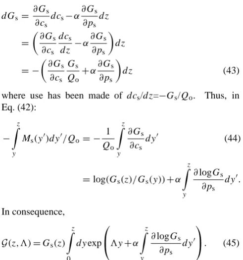
−t/t is the exponential integral. Figure 1a plotsPsas a function of Qofor two values ofβ. For sufficiently high value ofβ,Ps exhibits two increasing branches connected by a decreasing branch. Letβ* be the critical value ofβ above which these three branches exist.
β* is found from the conditiondPs/dQo=d2Ps/dQ2o=0 to beβ*=2.989.
The frequency equation is taken from Eq. (46) with
∂Gs/∂ps=0. It reads:
ε−1+Q2o3eβ[Ei(−β)−Ei(−βe−1/Qo)] −Qo{exp[β(1−e−1/Qo)] −1}
−Qoeββ−Qo3[0(1+Qo3,β)−0(1+Qo3,βe−1/Qo)] =0 (50) where 0(a,x)≡R∞
x z
a−1e−tdt is the incomplete Gamma function. From this expression, it is straightforward to ob-tain the Hopf bifurcation curve εH, an example of which is illustrated in Fig. 1b for β=5.5. The vertical dotted lines correspond to the two values Qo* of Qo for which
dPs/dQo|Qo∗=0. In fact, it is easy to show analytically fromPs=Qoµand from Eq. (47) (in the limit→0)that the boundaries of the Hopf bifurcation curve are bounded byQo*. This is true for an arbitrary growth rateGof the form (34) and it shows an important property: a necessary condition for a Hopf bifurcation to exist is to haveβ > β* and to choose a value of Qo for which the corresponding
Ps(Qo)lies on a decreasing branchdPs/dQo<0. However, in contrast to what was suggested in Wylie et al. (1999), this not a sufficient condition: εmust be sufficiently large (ε > εH)for an instability to occur.
Fig. 1. (a) Steady state overpressurePsas a function of the flow rate
Qoat the base of the conduit for the WVW bubble growth model, for two values of the viscosity response coefficientβ. As discussed in Appendix B, the path ABCD describes the oscillatory cycle in (P,Q)space obtained in the limit whereε→ ∞. (b) Steady state stability phase diagram in parameter space (Qo,ε)forβ=5.5 for the WVW bubble growth model. S=stable node; SF=stable focus; U=unstable focus. The Hopf bifurcation line (continuous curve) resides within the region where the steady statePs(Qo)exhibits two extrema (dashed vertical lines).
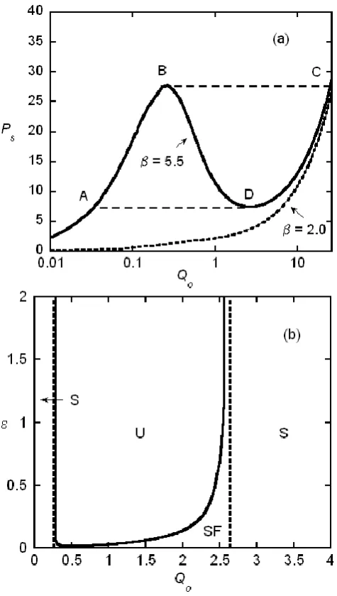
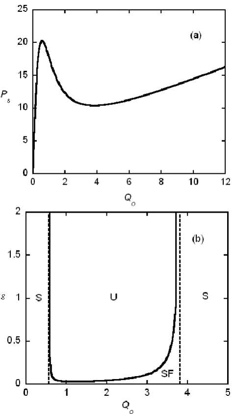
a Hopf bifurcation curve for the two growth models, respec-tively. The choice of parameter values is discussed in the next section. For this choice, the critical values ofβ* are 2.60 for the SBG model and 3.75 for the MBG model. Although the details are quantitatively different from the WVW case, the topology of the curves is identical.
Fig. 2. (a) Steady state overpressurePs as a function of the flow rateQoat the base of the conduit for the SBG model withβ=5.5. (b) Steady state stability phase diagram in parameter space (Qo,
ε) forβ=5.5 for the SBG bubble growth model. S=stable node; SF=stable focus; U=unstable focus. The Hopf bifurcation line (continuous curve) resides within the region where the steady state
Ps(Qo)exhibits two extrema (dashed vertical lines).
Fig. 3. (a) Steady state overpressurePsas a function of the flow rateQoat the base of the conduit for the MBG model withβ=5.5. (b) Steady state stability phase diagram in parameter space (Qo,ε) forβ=5.5 for the MBG model. S=stable node; SF=stable focus; U=unstable focus. The Hopf bifurcation line (continuous curve) resides within the region where the steady statePs(Qo)exhibits two extrema (dashed vertical lines).
4 Numerical results and discussion
4.1 Numerical approach
In order to investigate the nature of the attractor in the un-stable regime, numerical solutions of the system (28, 29, 31) were generated. The overpressure Eq. (29) is solved by a second-order finite difference scheme in the time-like vari-ableτ of step sizeh:
Table 1. Parameter values used in the calculations of Sect. 4.2. These are typical of the Montserrat system (Wylie et al., 1999). The value ofβis estimated from the temperature and from the empirical relation (19) (Shaw, 1972). The value of Henry constantKH, the volatile diffusion constantDand the initial bubble radiusR(0) are taken from Proussevitch et al. (1993). The bubble number density
Nis inferred from Proussevitch et al. (1993).
Parameter Units Value
co Mass proportion 0.05
D m2/s 10−11
g m/s2 9.8
k s−1 2.77×10⁻⁴
KH Pa−1 1.6×10⁻¹¹
L m 400
M kg/mol 0.018
n – 1/2
N m−3 2.38×10⁸
pa Pa 101.32×10³
r m 10
R(0) m 10−5
To K 1173
β – 5.5
ρ kg/m3 2500
Pn+1=Pn+Qoh 2ε (1/Q
n+1/Qn+1)−h
ε (51)
wherePn andQndenote respectively the overpressure and the flow rate atτ=nhwithnan integer. The advection equa-tion (Eq. 28) is solved using an upstream explicit scheme. The step sizesh inz- andτ-space are chosen to be equal, so as to minimize numerical dispersion. Let cinandpni de-note the concentration and pressure fields at positionz=ih andτ=nh whereiis an integer. This algorithm gives
cni+1=cni−1−hG(cni,pni)(1/Qn+1/Qn+1)/2. (52) 1/Qn+1is chosen in a self-consistent manner (via a Newton-Raphson algorithm) so as to be consistent with the dis-cretized version of the integral constraint (31):
Pn+1/Qn+1−hX
i
wiexp[β(1−cni+1)] =0 (53)
wherewi are weight constants associated with the particu-lar numerical integration method used (withhsmall enough, a trapezoidal integration method was found to be suffi-cient).With the fieldcupdated, the full pressure field can be finally found by the numerical integration of Eq. (30). The algorithm is fast, simple and convergent.
4.2 Numerical solutions
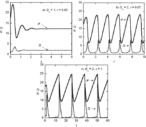
Fig. 4. Time seriesP (t ),Q(t )for the MBG model withβ=5.5. (a)Qo=2,ε=0.02; (b)Qo=2,ε=0.07; (c)Qo=2,ε=1.0. Parameters values as in Table 1. The initial condition has been chosen asQ(0)=1 with an initial pressure and concentration profiles that have the steady state form for this value ofQ(0).
With these parameter values, the time scalet¯is 1 h for the WVW model and 1.58 h for the SBG and the MBG mod-els. The scaled parameters areα=29.1, γ=14.2,δ=0.3 and
A=0.046. In the growth rate expressions, we have also used the approximation of Eq. (34) in order to verify the bifurca-tion analysis performed in Sect. 3.
Figure 4a illustrates for the MBG model an overpressure and flow rate time series in a regime wheredPs/dQo<0 but for a case where the steady state is stable (ε < εH). Figure 4b illustrates the corresponding time series whenεis just above
εH. In agreement with the analysis, the steady state is indeed unstable in the latter case. The solution evolves towards a stable limit cycle. Figure 4c illustrates a limit cycle obtained for a larger value ofε > εH. This illustrates that the pressure
cycle approaches a saw-tooth time-behavior and that the flow rate exhibits bursting. These features are typical and are sim-ilarly found in the two other growth models, WVW and SBG (not illustrated).
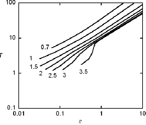
The cycle periodT (with respect to the time variablet )is a highly sensitive function ofQoandε. This is illustrated in Fig. 5 for the MBG growth model where each curve shows
T as a function ofεfor various values ofQo. The curves
T (ε)are similar for the two other growth models. In general,
Fig. 5. Cycle periodT as a function ofεfor the MBG model with
β=5.5 and for various values ofQo, as indicated on the curves. Parameters values as in Table 1.
easy to show that the period takes the asymptotic value (see Appendix B):
T ∼=ε
P
sB(QC−QB)
(Qo−QB)(QC−Qo)
− PsA(QD−QA) (Qo−QA)(QD−Qo)
− B
Z
A
Ps(Q)dQ
(Qo−Q)2 +
C
Z
D
Ps(Q)dQ
(Qo−Q)2
(54)
wherePs(Q)is the steady state overpressure curve and the labels A, B, C, D correspond to the boundary of the limit cy-cle in{P,Q}space, as shown, for instance, in Fig. 1a. The fact that that the period curves obtained from the numerical solutions go smoothly to its analytical asymptotic expression is a further indication of the adequacy of the numerical algo-rithm.
4.3 Comparison with observations: the Soufri`ere system
In this section, we present numerical results for the case where the full pressure expression is kept in the growth rate, so that the approximation (34) is relaxed. The general fea-tures of the solution are qualitatively identical as those de-scribed above. We will use this approach to see how the model applies to actual observations. For concreteness, we will consider the tilt angle measurements performed on the shallow Soufri`ere system in August 1997 (top of Fig. 5 in Voight et al., 1998). When the steady state is unstable, the asymptotic state of our model is a limit cycle with a well-defined period and amplitude. However, the observed peri-ods and oscillation amplitudes are not quite constant. This
Table 2. Values of the parameterεand the time scalet¯leading to a minimum in the error functioneof Eq. (55) for various bubble growth models. Here,Tobs=18 h andaobs=0.6. The dimensionless reservoir flow rateQ0ois calculated from Eq. (22) with the knowl-edge oft¯and assumingQo=10 m3/s. Also, T
calc= ¯t Tcalc0 . The productV ηois estimated from Eq. (22) with the knowledge oft¯and
ε, and assumingY=3×10¹⁰Pa andσ=0.2.1P is the amplitude of the overpressure drop over one cycle.1Qis the corresponding flow rate amplitude.χis defined in Eq. (56).
WVWa SBGb MBGc ¯
t(hours) 7.37 1.44 6.36
ε 0.20 1.30 0.34
Q0o 2.11 0.41 1.82
Tcalc(hours) 17.70 17.37 17.81
acalc 0.603 0.651 0.596
e(%) 1.73 9.17 1.34
V ηo(×105km3Pa-s) 6.51 8.26 9.56
1P /ηo(s−1) 1.53 1.80 1.20
1Q(m3/s) 8.9 15.6 10.3
χ 1.3 2.0 1.0
a Wiley-Voight-Whitehead;b Single-Bubble Growth; c Multiple-Bubble Growth
could be due to a combination of transient effects and/or sys-tematic slow or random variations in the system parameters which are not described by our simple model. Nevertheless, by requesting that the limit cycle solution is close to a typical measured cycle, our model can be used to obtain reasonable estimates of two of the parameter values that are not easily accessible: the time scale t¯and the dimensionless magma chamber elastic parameterε.
For the purpose of illustration, we selected the particu-larly well-defined cycle from 2 August to 3 August, which has a period Tobs=18 h and is characterized by a dimen-sionless asymmetry parameteraobs≡(tmax−tmin)/Tobs=0.6 wheretmax andtmin are the times at the cycle maximum or minimum, respectively. BothTobsandaobsdo not depend on the specific (possibly non linear) conversion between tilt an-gle measurements and overpressure values. We only need to assume that extrema in tilt angles occur at the same time as extrema in overpressure. From the limit cycle solutionsP (t ), we have adjustedt¯andεby minimizing the residual relative errore
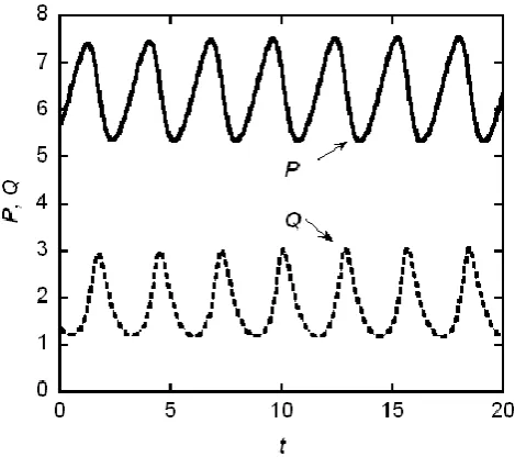
Fig. 6. Limit cycleP (t ),Q(t )for the MBG model withβ=5.5 and for values of the time scalet¯andεthat minimize the relative error
e(Table 2). The origin of the time axis is arbitrary as the transients are not illustrated.
values oft¯andε. The curves are qualitatively similar for the two other growth models. Nevertheless, the minimal residual error is about seven times larger for the SBG growth model than for the two other models.
Taking the estimates (Wylie et al., 1999)Y=3×10¹⁰Pa and
σ=0.2 with L, and r from Table 1, we obtain the product
V ηo from Eq. (22). This estimate is reported in Table 2. For comparison, the estimateV ηo=2.34×10⁵km3Pa-s is in-ferred from Wylie et al. (1999), with a time scale arbitrarily chosen ast¯=1 h. Table 2 also gives the ratio (in s−1)of the overpressure drop over a cycle,1P, by the viscosityηo. For
ηo=106Pa-s (Voight et al., 1999), the overpressure drop is of the order of the MPa, consistent with the observations. The table also gives the flow rate amplitude1Q in m3/s. Notwithstanding the difference in the values oft¯(which im-plies a difference in the pressure and flow rate scales), the amplitude of the variations1P and1Qare comparable for all three bubble growth rate models.
Assuming a linear scaling between the overpressureP at the base of the conduit and tilt angle measurements (Voight et al., 1999), the following chi-square
χ2=1 f
X
i
CPi+B−θi
σi
2
(56) can be estimated. Hereθiare measured tilt angles (from the 2–3 August cycle in Fig. 5 of Voight et al., 1998), B and
Care two constants defining the assumed linear relation be-tween the calculated (dimensionless) overpressurePiand the tilt angle.σi(estimated to be 10% ofθi)is the error on the tilt angle measurement andf the number of degrees of freedom.
We have selected the parameterst¯andεfrom Table 2. The values ofχare reported in Table 2. These values suggest that the SBG model does not provide a good fit, whereas both the MBG and WVW growth models lead to a marginally good fit (with a slightly better fit in favor of the MBG model). Never-theless, on physical grounds, one expects the bubble growth expression to have a more complex form than what Eq. (11) implies. Notwithstanding the large number of simplifying assumptions, the application of this model to data allows one to constraint the values of the time scalet¯and of the elastic response parameterε, which are not easily available other-wise.
5 Conclusion
In this contribution, we have extended the model of Wylie et al. (1999) describing a simple mechanism for the gener-ation of an oscillatory behavior in a shallow magmatic sys-tem. In this model, magma flow is coupled to the magma water content through the explicit volatile dependence of the melt viscosity. We have extended the original model by re-laxing three of its simplifying assumptions: use is made of an arbitrary volatile bubble growth rate law expression, we do not assume that the volatile concentration profile has a steady-state form and the spatial integral of the viscosity in Eq. (31) is properly evaluated. We have also performed a linear stability analysis of the system and have established that the oscillatory behavior occurs via a Hopf bifurcation. The range of parameter values for which oscillatory behav-ior exists have been found for three different bubble growth models: the linear growth model of Wylie et al., the single bubble diffusion-limited growth model and an approximate many-bubble growth model that has been recently published (L’Heureux, 2007). We have found that this modeling ap-proach can generate oscillatory magma dynamics with a pe-riod that is compatible with the observations. The quality of the fit with the observations can be used to constraint some system parameters that are not easily measured.
Appendix A
Notation and description of the variables
Notation Units Description
a – Asymmetry parameter (Eq. 55).
A – Scaled Henry constant in
Eq. (25).
B rad Constant in Eq. (56).
c – Dissolved volatile concentra-tion.
co – Value ofcat the base of the up-per conduit.
ceq – Equilibrium concentration.
ceq,o – Initial equilibrium concentra-tion.
C rad Constant in Eq. (56)
D m2/s Volatile diffusion coefficient.
e – Residual relative error in
Eq. (55).
f – Degree of freedom in Eq. (56).
g m/s2 Acceleration of gravity.
G s−1 Exsolution rate.
G – Factor relating δc to δQ in
Eq. (42).
h – τ step in the numerical imple-mentation.
J m−3s−1 Nucleation rate.
k s−1 Rate constant in WVW model.
K s−1 Rate constant in MBG model.
KH Pa−1 Henry constant.
L m Length of upper conduit.
m – Total volatile concentration.
M kg/mol Volatile molar mass.
N m−3 Bubble number density.
p Pa Total pressure.
pa Pa Atmospheric pressure.
po – Scaled initial pressure (Eq. 26).
P Pa Overpressure.
Q m3/s Magma flow rate.
Qo m3/s Input magma flow rate.
r m Radius of upper conduit.
R m Bubble radius.
R∞ m Large-time limit of the bubble radius (Eq. 18).
R J/K-mol Molar gas constant.
t s Time.
¯
t s Time scale.
To K Temperature.
T s Cycle period.
v m/s Radial bubble growth rate.
V m3 Volume of magma reservoir and lower conduit.
Notation Units Description
wi – Weights in the numerical inte-gration of Eq. (31).
Y Pa Young’s modulus.
z m Vertical coordinate with respect to the base of the upper conduit.
α – Scaled melt density (Eq. 22).
β – Viscosity response coefficient.
δ – Scaled atmospheric pressure
(Eq. 22).
δc,δP ,δQ – Variations ofc,P,Qabout their steady state.
ε – Scaled reservoir elastic response (Eq. 22).
εH – Value of εat the Hopf bifurca-tion point.
φ – Vesicularity.
γ – Constant in Eq. (26).
3 – Frequency of the perturbations of (c,P, Q)about their steady state.
η Pa-s Melt viscosity.
ηo Pa-s Melt viscosity at the base of the upper conduit.
µ – Integrated scaled viscosity
(Eq. 37).
θi rad Tilt angle.
ρ kg/m3 Melt density.
ρg kg/m3 Volatile density in the bubble phase.
σ – Poisson coefficient of the rock surrounding the system.
σi rad Error on tilt angle.
τ – Time-like variable (Eq. 27).
– Frequency of the cycle at the Hopf bifurcation point.
Appendix B
Cycle period in the largeεlimit
In this Appendix, we show that the period of the oscillatory solution in the limit of largeεis given by Eq. (54). Perform-ing a change of time scaleτ→ετ0in Eq. (28) and taking the limit ε→ ∞indicate that the concentration profile relaxes quickly to a pseudo-steady state form similar to Eq. (33), except thatQois replaced by the slowly varying flow rate
Q(τ0). One recalls that the overpressure at the base of the magma conduit is given by Eq. (31) (P (τ0)=Q(τ0)µ(τ0))
fromQo, the pressure cycle is described by a slow motion along the ascending branches of steady state diagrams such as those of Figs. 1a, 2a or 3a. The overpressure slow dynam-ics is described by Eq. (29):
dP dτ0=
Qo−Q(τ0)
Q(τ0) . (B1)
Thus it is seen that the pressure can not assume values on the decreasing branch of the steady state diagram(where
dPs/dQo<0). Rather, the motions along the two ascend-ing branches are connected by horizontal lines joinascend-ing B to C and D to A in Fig. 1a, resulting in very fast variations in
Q(τ0). To calculate the cycle periodT, we rewrite Eq. (B1) as εdP /dt=Qo−Q where we useddτ/dt=Q (Eq. 27). The period is then:
T=ε
I dP
Qo−Q =ε
B
Z
A
dP Qo−Q
+ε
D
Z
C
dP Qo−Q
(B2)
where we neglected the time used to run along the horizontal paths BC and DA. Integrating by parts with respect toQwith
P=Ps=Qµsfinally gives Eq. (54).
Acknowledgements. This research was supported by a grant from the Natural Sciences and Engineering Research Council of Canada. The author acknowledges fruitful discussion with Anthony D. Fowler and the assistance of Maria Stefanescu.
Edited by: S. Lovejoy
Reviewed by: A. G. Hunt and another anonymous referee
References
Barmin, A., Melnik, O., and Sparks, R. S. J.: Periodic behavior in lava dome eruptions, Earth Planet. Sci. Lett., 199, 173–184, 2002.
Behrens, H. and Gaillard, F.: Geochemical aspects of melts: Volatiles and redox behavior, Elements, 2, 275–280, 2006. Bottinga, Y. and Javoy, M.: Mid-ocean ridge basalt degassing:
Bub-ble nucleation, J. Geophys. Res., 95, 5125–5131, 1990. Burnham, C. W.: Water in magmas: A mixing model, Geochim.
Cosmochim. Act., 39, 1077–1084, 1975.
Clemens, J. D. and Petford, N.: Granitic melt viscosity and silicic magma dynamics in contrasting tectonic settings, J. Geol. Soc. (London), 156, 1057–1060, 1999.
Costa, A. and Macedonio, G.: Nonlinear phenomena in flu-ids with temperature-dependent viscosity: An hysteresis model for magma flow in conduits, Geophys. Res. Lett., 29, 1402, doi:10.1029/2001GLO14493, 2002.
Costa, A., Melnik, O., Sparks, R. S. J., and Voight, B.: Control of magma flow in dykes on cyclic lava dome extrusion, Geophys. Res. Lett., 34, L02303, doi:10.1029/2006GL027466, 2007. De Vivo, B., Lima A., and Webster, J. D.: Volatiles in
magmatic-volcanic systems, Elements, 1, 19–24, 2005.
Harris, A. J. L., Rose, W. I., and Flynn, L. P.: Temporal trends in lava dome extrusion at Santiaguito 1922–2000, Bull. Volcanol., 65, 77–89, 2003.
Hess, K.-U. and Dingwell, D. B.: Viscosities of hydrous leucogranitic melts: a non- Arrhenian model, Amer. Mineral., 81, 1297–1300, 1996.
Landau, L. D. and Lifshitz, E. M.: Theory of Elasticity, Pergamon Press, Oxford, 1970.
L’Heureux, I.: A new model of volatile bubble growth in a mag-matic system: Isobaric case, J. Geophys. Res., 112, B12208, doi:10.1029/2006JB004872, 2007.
Mader, H. M.: Conduit flow and fragmentation, in: The Physics of Explosive Volcanic Eruptions, edited by: Gilbert, J. S. and Sparks, R. S. J., Special Publication no. 145, Geol. Soc., London, 27–50, 1998.
Marqusee, J. A. and Ross, J.: Theory of Ostwald ripening: Com-petitive growth and its dependence on volume fraction, J. Chem. Phys., 80, 536–543, 1984.
Melnik, O. and Sparks, R. S. J.: Nonlinear dynamics of lava dome extrusion, Nature, 402, 37–41, 1999.
Melnik, O. and Sparks, R. S. J.: Controls on conduit magma flow dynamics during lava dome building eruptions, J. Geophys. Res., 110, B02209, doi:10.1029/2004JB003183, 2005.
Mourtada-Bonnefoi, C. C., Provost, A., and Albar`ede, F.: Ther-mochemical dynamics of magma chambers: A simple model, J. Geophys. Res., 104, 7103–7115, 1999.
Nakada, S., Shimizu, H., and Ohta, K.: Overview of the 1990–1995 eruption at Unzen Volcano, J. Volcanol. Geotherm. Res., 89, 1– 22, 1999.
Navon, O. and Lyakhovsky, V.: Vesiculation processes in silicic magmas, in: The Physics of Explosive Volcanic Eruptions, edited by: Gilbert, J. S. and Sparks, R. S. J., Special Publication no.145, Geol. Soc., London, 27–50, 1998.
Nakanishi, M. and Koyaguchi, T.: A stability analysis of a conduit flow model for lava dome eruptions, J. Volcanol. Geotherm. Res., 178, 46–57, 2008.
Ozerov, A., Ispolatov, I., and Lees, J.: Modeling Strombolian erup-tions of Karymsky volcano, Kamchatka, Russia, J. Volcanol. Geotherm. Res., 122, 265–280, 2003.
Proussevitch, A. A., Sahagian, D. L., and Anderson, A. T.: Dynam-ics of diffusive bubble growth in magmas: Isothermal case, J. Geophys. Res., 98, 22283–22307, 1993.
Proussevitch, A. A. and Sahagian, D. L.: Dynamics of coupled dif-fusive and decompressive bubble growth in magatics systems, J. Geophys. Res., 101, 17447–17455, 1996.
Proussevitch, A. A. and Sahagian, D. L.: Dynamics and energetics of bubble growth in magmas: Analytical formulation and numer-ical modeling, J. Geophys.Res., 103, 18223–18251, 1998. Shaw, H. R.: Viscosities of magmatic silicate liquids: an empirical
method of prediction, Amer. J. Sci., 272, 870–893, 1972. Sparks, R. S. J.: The dynamics of bubble formation and growth in
magmas: A review and analysis, J. Volcanol. Geotherm. Res., 3, 1–37, 1978.
Sparks, R. S. J. and Young, S. R.: The eruption of Soufri`ere Hills volcano, Montserrat (1995–1999): Overview of scientific results, Mem. Geol. Soc., 21, 45–69, 2002.
British West Indies, Science, 283, 1138–1142, 1999.
Voight, B., Constantine, E. K., Siswowidjoyo, S., and Torley, R.: Historical eruptions of Merapi Volcano, central Java, Indonesia, 1768–1998, J. Volcanol. Geotherm. Res., 100, 69–138, 2000. Wiesenfeld, K.: Noisy precursors of nonlinear instabilities, J. Stat
Phys., 38, 1071–1097, 1985.