www.atmos-meas-tech.net/9/5077/2016/ doi:10.5194/amt-9-5077-2016
© Author(s) 2016. CC Attribution 3.0 License.
Application of the full spectrum inversion algorithm
to simulated airborne GPS radio occultation signals
Loknath Adhikari1, Feiqin Xie1, and Jennifer S. Haase2
1Department of Physical and Environmental Sciences, Texas A & M University – Corpus Christi, Corpus Christi, TX, USA 2Scripps Institution of Oceanography, University of California, San Diego, La Jolla, CA, USA
Correspondence to:Loknath Adhikari ([email protected])
Received: 4 December 2015 – Published in Atmos. Meas. Tech. Discuss.: 18 January 2016 Revised: 29 August 2016 – Accepted: 20 September 2016 – Published: 18 October 2016
Abstract. With a GPS receiver on board an airplane, the airborne radio occultation (ARO) technique provides dense lower-tropospheric soundings over target regions. Large vari-ations in water vapor in the troposphere cause strong signal multipath, which could lead to systematic errors in RO re-trievals with the geometric optics (GO) method. The space-borne GPS RO community has successfully developed the full-spectrum inversion (FSI) technique to solve the multi-path problem. This paper is the first to adapt the FSI tech-nique to retrieve atmospheric properties (bending and refrac-tivity) from ARO signals, where it is necessary to compen-sate for the receiver traveling on a non-circular trajectory in-side the atmosphere, and its use is demonstrated using an end-to-end simulation system.
The forward-simulated GPS L1 (1575.42 MHz) signal am-plitude and phase are used to test the modified FSI algorithm. The ARO FSI method is capable of reconstructing the fine vertical structure of the moist lower troposphere in the pres-ence of severe multipath, which otherwise leads to large re-trieval errors in the GO rere-trieval. The sensitivity of the mod-ified FSI-retrieved bending angle and refractivity to errors in signal amplitude and errors in the measured refractivity at the receiver is presented. Accurate bending angle retrievals can be obtained from the surface up to ∼250 m below the re-ceiver at typical flight altitudes above the tropopause, above which the retrieved bending angle becomes highly sensitive to the phase measurement noise. Abrupt changes in the sig-nal amplitude that are a challenge for receiver tracking and geometric optics bending angle retrieval techniques do not produce any systematic bias in the FSI retrievals when the SNR is high. For very low SNR, the FSI performs as expected from theoretical considerations. The 1 % in situ
refractiv-ity measurement errors at the receiver height can introduce a maximum refractivity retrieval error of 0.5 % (1 K) near the receiver, but the error decreases gradually to ∼0.05 % (0.1 K) near the surface. In summary, the ARO FSI success-fully retrieves the fine vertical structure of the atmosphere in the presence of multipath in the lower troposphere.
1 Introduction
con-servative quantity for each signal ray. The tangent point is the point along a ray path where the radius vector from the center of curvature is normal to the ray, and it is the closest point on the ray path to the Earth surface. The bending angle can then be converted to refractivity through the inverse Abel trans-formation (Fjeldbo et al., 1971). The refractivity (N) or the refractive index (n) of the neutral atmosphere depends on the atmospheric temperature (T in Kelvin), total pressure (P in hPa), and water vapor pressure (ein hPa) (Kursinski et al., 1997, 2000), as follows:
N =(n−1)×106=77.6P
T +3.73×10
5 e
T2. (1) The fundamental observations made during an ARO event are the time series of phase and signal-to-noise ratio (SNR) of the RO signals. After the precise positions of the GPS and the receiver are known (e.g., Muradyan et al., 2010), the excess phase delay due to atmospheric refraction can be derived by differencing the measured signal total phase (with some initial ambiguity) with the GPS–receiver line-of-sight (LOS) distance. In this study we simulate GPS L1 sig-nals (1575.42 MHz) for an airborne receiver at 14 km. We neglect ionospheric effects, which can be removed through the linear combination of dual frequency measurements (e.g., Vorobev and Krasil’nikova, 1994; Hajj et al., 2002). Iono-spheric errors dominate spaceborne RO retrievals above 30 km (Kursinski et al., 1997); however, ARO retrievals are not possible above the height of the aircraft. In the-ory, the ionospheric effects are negligible for ARO retrievals in a spherically symmetric atmosphere, because the ARO retrieval requires the differencing between the RO signals originating from below (negative elevation angle) and above (positive elevation angle) the local horizon, which will cancel out most of the ionospheric errors (Xie et al., 2008) (hereafter referred to as X08). In practice, the largest part of the iono-spheric error is compensated by an initial code delay in the closed-loop tracking before transitioning to open-loop track-ing, and the remaining decrease in ionospheric delay (ad-vance) over the course of the occultation is much smaller than the neutral delay (Wang et al., 2016) and other error sources. This will minimize the need for dual GPS frequency ARO measurements. The partial bending angle, defined as the dif-ference between the bending angle measurements at the neg-ative elevation and the bending at the positive elevation, cor-responding to the same impact parameter, is then used to derive the refractivity through the inverse Abel transform. The derivative of the excess phase represents the Doppler shift of the carrier signal. The commonly used geometric op-tics (GO) method uses the measured Doppler and the GPS– receiver positions and velocities to retrieve the bending angle (Vorobev and Krasil’nikova, 1994). One major limitation of the GO method is its inability to account for signal interfer-ence, known as multipath, that frequently occurs in the moist lower troposphere due to sharp water vapor gradients. When multipath occurs, the signal at the receiver at a given time
consists of the superposition of multiple rays, each having a unique impact parameter, and the Doppler shift derived from the signal phase no longer corresponds to a unique ray path with one impact parameter. As a result, the GO method can lead to large retrieval errors.
Various radio holographic methods have been proposed to overcome the limitations of the GO method in the spaceborne RO retrievals (e.g., Gorbunov et al., 1996; Gorbunov and Gurvich, 1998; Sokolovskiy, 2001; Gorbunov, 2002; Jensen et al., 2003, 2004; Gorbunov and Lauritsen, 2004). The full-spectrum inversion (FSI) proposed by Jensen et al. (2003) (hereafter referred to as J03) has been applied to invert space-borne RO signals and outperforms the GO method in the presence of multipath. However, prior to this work it had not been implemented for airborne RO because of the need to ad-dress the unique characteristics of ARO occultation measure-ments. In particular, due to the the asymmetry of the ray path from GPS to a receiver inside the atmosphere, ARO retrieval requires additional measurement of RO signals above the lo-cal horizon. Moreover, the irregular (non-circular) flight path of the airborne platform must also be taken into account.
This paper is organized as follows: Sect. 2 describes the key implementation steps for the FSI method for ARO. An end-to-end simulation system is presented in Sect. 3. Sec-tion 4 presents simulated ARO observaSec-tions under severe multipath conditions, where the FSI is expected to provide major improvement. The sensitivity of the FSI retrievals to the ARO measurement errors in signal amplitude and the re-fractivity at the receiver are explored in Sect. 5. The conclu-sions are summarized in Sect. 6.
2 Theoretical derivation of FSI for airborne RO measurements
The FSI method operates directly on the measured signal along the receiver trajectory, recognizes the recorded RO sig-nal as radio waves of different frequencies determined by the refractive index of the media through which they pass, and accounts for interference of waves with different frequen-cies. In contrast, the GO retrieval does not account for the possible superposition in time of multiple waves. Jensen et al. (2003) demonstrated that the derivative of the phase of the Fourier transform of the measured signal as a function of open angle distinguishes the different frequency components by using the method of stationary phase (MSP). The open angle (θ) is defined as the angle between the two radius vec-tors from the center of curvature to the GPS transmitter and the airborne receiver. Therefore, the time series of phase and amplitude must be resampled with respect to equally spaced open angle rather than time. For a realistic occultation with an oblate Earth and non-coplanar near-circular trajectories for the GPS and the receiver, a correction must also be ap-plied to the observed phase to project the observations onto circular trajectories. In the case of ARO, the GPS time series is split into two parts, corresponding to the positive and neg-ative elevation angle measurements. Each time segment can then be separately processed with the FSI.
The GPS signal composed of several narrowband subsig-nals resampled with respect toθcan be expressed as
u(θ )=X p
Ap(θ )eiϕp(θ ), (2)
whereApandϕpare the amplitude and phase of thepth sub-signal, whose Fourier transform can be expressed as
F ωˆ=X p
θ2 Z
θ1
Ap(θ0)ei(ϕp− ˆω
0
)dθ0, (3)
whereθ1andθ2are the open angles at the beginning and the end of occultation, respectively.
The MSP assumes that at an instantaneous pseudo fre-quency in the Fourier integral in Eq. (3) is dominated by the contribution from a single subsignal near the stationary point (Born and Wolf, 1999). Equation (3) can then be simplified to Eq. (4):
F ωˆ≈
Bei(ϕq− ˆωqθs), (4)
where B is amplitude that is approximately constant and ˆ
ωq is the pseudo frequency corresponding to the subsignal at the stationary phase that satisfies
ˆ
ωq=
dϕq
dθ |θ=θs. (5)
The derivative of the phase (ψ=ϕq− ˆωqθs) of the Fourier transform with respect toωˆ gives the open angle (θs) that corresponds to the pseudo frequency, i.e.,
θs= −
dψ
dωˆ. (6)
Using the propagation path of a ray from the transmitter to the receiver, which corresponds to the individual subsignalq
mentioned above, it can be shown following Appendix A of J03 that the derivative of the phase (φq) of the subsig-nal with respect toθ(the pseudo frequencyωˆq) for the ARO signal can be expressed as
dϕq
dθ = ˆωq=ka±k dRrec
dθ
s 1−
a
nrecRrec
2
+kdRGPS dθ
s 1−
a RGPS
2
, (7)
wherek,a,nrec,Rrec, and RGPS are respectively the wave number of the GPS L1 carrier signal, impact parameter, re-fractive index at the receiver, radius of receiver, and radius of GPS from the center of the Earth. With the ARO receiver lo-cated within the atmosphere, the difference between Eq. (7) above and Eq. (13) in J03 arises from the inclusion of the refractive index at the ARO receiver (nrec), which is greater than 1 and is a function of receiver position. Similar to the the spaceborne RO case with receivers outside the Earth’s neutral atmosphere and only measuring at negative elevation angle, the sign of the second term in Eq. (7) is positive at negative elevation angle, but it becomes negative at positive elevation angle when the ARO receiver and the transmitter are located on the same side of the tangent point. Note that Eq. (7) is derived from the calculation of the path length of a signal ray. Therefore, at positive elevation, the tangent point to the receiver path length should be subtracted from the tan-gent point to GPS path length to get the total path length.
The last two terms in Eq. (7) are frequency changes caused by the radial variations due to the non-circular trajectories of the GPS and the receiver, which will be removed through a correction described in the following section. When both trajectories are circular, the equation can be simplified to
dϕq
which shows that the pseudo frequency is proportional to the impact parameter of the subsignal when the GPS and the re-ceiver travel in a circular orbit.
After identifying the contribution from individual subsig-nals, these can be attributed to distinct ray paths, and sub-sequently the impact parameter (a) can be derived based on Eq. (8). Note that the impact parameter (a) of a ray is defined as (Kursinski et al., 1997)
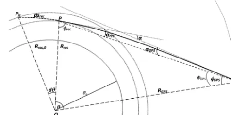
a=nGPSRGPSsinφGPS=nrecRrecsinφrec, (9) whereφGPSandφrecare the angle between the ray tangential direction and the radius vector at the GPS and the receiver, respectively (see Fig. 1). Using Eq. (9) and takingnGPS=1 at the GPS position, the angleφGPScan be calculated as
φGPS=arcsin
a RGPS
. (10a)
In the case of ARO,φrec=π/2 refers to the local horizon or zero elevation angle, whereas φrec> π/2 refers to the posi-tive elevation angle andφrec< π/2 refers to the negative ele-vation angle (see X08 for detailed description of positive and negative elevation angles). Therefore, φrec for positive and negative elevation angles are given by Eqs. (10b) and (10c), respectively as
φrec=π−arcsin
a nrecRrec
, (10b)
φrec=arcsin
a nrecRrec
. (10c)
The derivative of Eq. (8) gives
da=1
kdω.ˆ (11)
The value ofdωˆis the spectrum resolution (Fowles, 1989) of the phase of the Fourier transform and is given by
dωˆ= 2π
1θ, (12)
where1θ=θ2−θ1is the difference in the open angle from the start to the end of the occultation.
The open angle can be computed using Eq. (6). The bend-ing angle (α)can then be calculated using
α=θ+φrec+φGPS−π. (13) Subsequently, the refractivity profile as a function of geomet-ric height can be derived using the inverse Abel transforma-tion (see X08 and Healy et al., 2002, for details).
2.1 Correction for non-spherical trajectory
The FSI retrieval equations in the preceding section are de-rived assuming a circular orbit of the GPS and the receiver
Figure 1.Schematic plot of airborne radio occultation geometry.
Projection of the receiver from its original position P with
ra-diusRreconto a new positionP0on a circular trajectory with
ra-diusRrec,0 relative to local center of curvatureO. The radius of
curvature,Re, is shown as a solid black line.
relative to the center. When the GPS and the receiver trajecto-ries become non-circular, the radial velocity terms in Eq. (7) are nonzero.
In real airborne occultation measurements, the perfectly circular trajectory assumption is not valid in part because of the oblateness of the Earth, as well as any height variations of the receiver. In addition, the asymmetry of the ray path from the source to a receiver inside the atmosphere requires additional measurement of RO signals above the local hori-zon and correction for the irregular (non-circular) flight path of the airborne platform. To take into account the oblateness of the Earth, Syndergaard (1998) showed that the inversion of the RO data should be performed assuming local spherical symmetry tangential to the Earth’s ellipsoid.
tri-angle formed by joining the origin,O, withP and the point where the direction vector atP intersects the reference circu-lar trajectory with radiusRrec,0. The value ofRrec,0is taken as the highest receiver altitude for the duration of the occul-tation and is a constant. However, the atmospheric medium betweenP and the projected position P0 causes additional bending of the ray path, which can be estimated from
Rrecnrecsinφrec=Rrec,0nP0sinφrec,0, (14) wherenP0 is the refractivity at the projected point,P0.
In practice, the additional phase resulting from the bend-ing fromP toP0is estimated as the straight line projection multiplied by the mean refractive index (nrec), obtained from the CIRA+Q refractivity climatological model, between the original position and the projected position. The correction using a straight line approximation is sufficient at the height of the aircraft (∼14 km) because the vertical refractivity gra-dients are small at these heights and do not induce signifi-cant bending until approximately 6–7 km in the troposphere (Murphy et al., 2015). As shown in the figure, this projec-tion from posiprojec-tion P to P0 leads to a change in the total phase (s), zenith angle (φ), and open angle (θ). The changes in phase (dsrec) and the open angel (dθrec) at the receiver can be calculated as
dsrec=nrec −Rreccosφrec± r
Rrec2 cos2φrec+
Rrec,02 −R2rec
!
, (15)
dθrec=arcsin
dsrecsin
Rrec
Rrec,0
. (16)
Since the GPS is located outside the Earth’s atmosphere, the refractive index at the GPS altitude is 1. Therefore, the cor-responding change in phase at the GPS (dsGPS) is given by
dsGPS= −RGPScosφGPS± r
R2
GPScos2φGPS+
R2
GPS,0−RGPS2
. (17)
The total phase after projection then becomes
s=s0+dsrec+dsGPS, (18) wheres0is the simulated phase atP0before the projection. The excess phase (se) can then be defined as
se=s−d, (19)
whered is the geometric phase, i.e., the GPS–receiver LOS distance. Note that the excess phase is used to calculate the excess Doppler used in the GO retrievals.
After the projection at each sample time, the new trajec-tories of both GPS and receiver are circular relative to the local center of curvature, and bothRrec,0andRGPS,0are con-stants, so the two radial terms in Eq. (7) become zero. No adjustment is made to the signal amplitude because the at-mospheric attenuation at these heights over short distances is insignificant. After the adjustment, FSI is applied to the
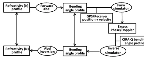
Figure 2.End-to-end simulation system for airborne RO data
pro-cessing. (Note: derivation of bending from refractivity in forward Abel does not need the occultation geometry information but only the receiver height and refractivity at the receiver.)
modified signal phase and the original signal amplitude with both GPS and receiver on circular trajectories. An alterna-tive method for correcting to a spherical orbit is to apply a Doppler shift (as in J03) or a diffraction correction (Gor-bunov and Lauritsen, 2004); however the phase correction in the time domain is the most straightforward to apply to the irregular flight trajectories of the research aircraft.
2.2 Estimation of the bending angle at the local horizon
In the case of airborne RO measurements, the bending an-gle is not a unique function of the impact parameter (a). The samea occurs twice, once each at negative and positive el-evation angle relative to the local horizon whereφrec=π/2 as seen in Fig. 1 (Zuffada et al., 1999; Healy et al., 2002). To avoid the non-unique relation betweenaand bending angle, the GPS total phase time series is split into two parts, i.e., the positive and negative elevation angle measurements. The FSI retrieval is then applied to each part separately. The time epoch when the occulting GPS is at the local horizon rela-tive to the ARO receiver (i.e., the separation point between positive and negative elevation angles) is estimated by ray-tracing through the CIRA+Q refractivity model to get the total bending angle (α) andaat each epoch. The time epoch whena reaches a maximum was selected as the separation between positive and negative elevation angle. The effect of any small time shift due to differences between the real atmo-sphere and the CIRA+Q climatological model will be min-imized when the time series is tapered prior to the Fourier transform.
3 End-to-end simulation system for airborne RO soundings
given an atmospheric refractivity model and occultation ge-ometry. The inverse simulator (or retrieval component) pro-cesses the simulated ARO signal phase and amplitude to re-trieve the atmospheric bending angle and refractivity profiles. 3.1 Forward ARO simulator (full-spectrum forward,
FSF)
Two different types of forward simulators were used in the study. The first option is a ray tracer that simulates the ARO signals as geometric optics rays (e.g., Xie et al., 2008). The initial ray direction from the transmitter is iteratively per-turbed until the ray is found that reaches the receiver. For-ward simulation using the ray-tracing technique becomes problematic when the atmosphere has sharp refractivity gra-dients. If the phase fluctuates rapidly for small perturbations in initial ray direction, the technique will not converge and cannot find a ray path connecting the GPS and receiver. Of-ten this occurs when there are multiple solutions (rays) for a given GPS-to-receiver geometry, i.e., atmospheric multipath. The second type of forward simulator that is used to simu-late the GPS signal in the presence of sharp refractivity gra-dients is a two-step procedure that combines an Abel integral forward model followed by a FSF simulator based on J03. The refractivity profile is input to the forward Abel integral (e.g., Fjeldbo et al., 1971; Xie et al., 2008), which calculates the bending as an integral function of radius from the sur-face to the aircraft height and GPS transmitter height. The resulting bending angle profile,α(a), which is geometry in-dependent, is then related to the given source-receiver geom-etryθ (a)using Eqs. (10) and (13). The bending angle profile as a function of the impact parameter and the correspond-ing θ (a) are the input atmospheric conditions to this FSF forward model to produce simulated phase and amplitude as a function of time.
The complex signal after Fourier transform in Eq. (4) can be expressed as a function ofaas follows:
F (a)≈B0(a)eiψ (a), (20) whereB0(a)can be approximated as a constant.
Each pseudo frequency corresponds to a single ray path having a unique impact parameter (a). As the pseudo fre-quency is proportional to the impact parameter as shown in Eq. (8), the derivative of the phase (ψ=ϕq− ˆωqθs) with re-spect to the impact parameter yields
dψ
da = −kθs. (21)
Therefore, the phase function ψ (a) of the Fourier-transformed occultation signals can be obtained by integrat-ing Eq. (7):
ψ (a)= −k
a2 Z
a1
θ (a)da+C, (22)
wherea1anda2are the impact parameters at the beginning and start of the occultation, andCis an unknown constant.
In this FSF forward model, the input atmospheric condi-tion is represented by a bending angle profile. Givenα(a), the θ (a) can be calculated using Eqs. (10) and (13). The phase function ψ (a) and thus F (a) can be be calculated through Eqs. (22) and (20), respectively.
Therefore, the complex occultation signal phase and am-plitude can be constructed through the inverse Fourier trans-form ofF (a), which can then be expressed as
u(θ )= a2 Z
a1
F (a)e−ikaθ (a)da. (23)
The complex signal, u(θ ), after the inverse Fourier trans-form, has a spectral resolution inθgiven by k(a2π
2−a1). The phase,φ (θ ), of the complex signal represents the total phase of the carrier signal with wave numberk plus an un-known constantCfrom Eq. (22). The signal amplitude,A(θ ), is calculated as the sum of the conjugate components of the complex signal. The pair (A(θ ),φ (θ )) and the correspond-ingθare thus evaluated from the inverse Fourier transform of the complex GPS signal in the impact parameter domain.
Subsequently, the excess phase as a function of the open angleθ, with an unknown constant, can be calculated by sub-tracting the LOS distance between GPS and receiver. Given the known occultation geometry for the GPS and the receiver, the relationship between the time andθcan then be applied to convert the excess phase into time space. The complex signal can therefore be generated through this full-spectrum forward operator, which eliminates the limitation of the geo-metric optics ray-tracing technique in the presence of multi-path.
3.2 Inverse ARO simulator (FSI)
Vapor mixing ratio (g kg–1)
Ex
cess doppler (m s
–1)
Heigh
t (k
m)
Impac
t heigh
t–R
ear
th
Tangen
t heigh
t (k
m)
Tangen
t heigh
t (k
m)
A
mplitude
Ex
cess phase (m)
Refractivity (N – unit) Refractivity error (%) Bending angle (°)
Temperature (°C) Time (s) Time (s)
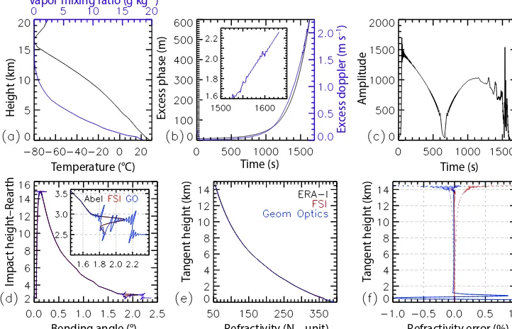
Figure 3. (a)ERA-I temperature and water vapor mixing ratio at 18:00 UTC on 13 September 2010 at 16.5◦N, 76.5◦W;(b)simulated
excess phase and derived Doppler velocity (inset shows the Doppler velocity after 1500 s);(c)simulated signal amplitude;(d) bending
angles retrieved using GO and FSI, and simulated bending observation with ERA-I refractivity profile (inset shows the close-up of the profile
near the surface);(e)refractivity profiles from GO, FSI retrievals and the ERA-I;(f)fractional refractivity error of GO (blue), and FSI (red)
compared to ERA-I. Dashed and solid lines are respectively for refractivity retrievals before and after the simple exponential atmospheric model near the receiver is applied.
4 Application of the FSI retrieval for simulated ARO measurements
To assess the performance of the ARO FSI retrieval algo-rithm, we used the occultation characteristics from an ac-tual aircraft flight and the atmospheric profile of tempera-ture and water vapor from the ERA-Interim reanalysis at the flight location and time. One specific occultation involves the GPS satellite PRN24 (the pseudo-random number identifies the satellite) and the airborne receiver during the PREDICT flight from 18:20 to 19:00 UTC on 14 September 2010 (re-search flight no. 19). In the simulation, the radius of the cur-vature of the Earth was found at the occultation location; then the aircraft height was set to a constant 14 km to produce an occultation geometry with a circular orbit for the receiver at the time when PRN24 was setting. The radius of the GPS orbit was set to a constant 26 000 km above the center of cur-vature. The grid profiles of ERA-I temperature and water va-por mixing ratio and the calculated refractivity profiles from the ARO sounding region are shown in Fig. 3a and e, respec-tively. Very moist atmospheric conditions with high mixing ratio (∼20 g kg−1) are seen near the surface, and moisture decreases rapidly at higher altitude; e.g., at 10 km, the tem-perature reduces to around 250 K (−23.15◦C). Observations from these flights showed that the contribution of water vapor to atmospheric refractivity becomes negligible in comparison
to that of temperature above a height of about 9 km (Murphy et al., 2015). Figure 3b shows the excess phase and excess Doppler obtained from the FSF forward simulator, where the initial time is referenced to zero when the open angle is 66.7◦, at∼5◦ elevation angle. The excess phase increases mono-tonically as a function of time, whereas its derivative, the excess Doppler, becomes a non-monotonic function of the time starting at∼1500 s (see inset figure). Such behavior in Doppler is a strong indication of signal interference due to multipath. The multipath is further illustrated by the time se-ries of the signal amplitude in Fig. 3c, which shows large variations around 1500 s. This signal amplitude variation is caused by superposition of multiple signals with varying fre-quencies.
and taper reduce the amplitude at the separation of the two ta-pered segments (Fig. 3c); therefore small errors in determin-ing the exact time (θ) separating positive and negative ele-vation angle due to the assumed CIRA+Q refractivity model have little effect on the FFT. In real observations this tapering will reduce the influence of observations at zero elevation an-gle, which in any case is constrained by the in situ refractivity observations.
The bending angle retrievals from GO (blue) and FSI (red) are plotted in Fig. 3d along with the “true” bending angle profile (black) from the Abel integral forward simulation. Two distinct and important features of the ARO retrievals are shown. The first is the large error in the retrieved bend-ing angle near zero elevation when the tangent point is near the receiver. This feature is present for both the GO and FSI methods. There is a singularity in both the GO and FSI re-trievals near zero elevation angle where small errors in ray tangent angle (near π/2) can result in large bending angle errors (e.g., Eqs. 10 and 13). In the case of FSI retrievals, there can be an additional error near the receiver height due to any uncertainties in the phase correction during the pro-jection from the non-spherical trajectory to the spherical tra-jectory in Eq. (15). However, this is resolved by knowing the refractivity at the receiver height, and hence impact pa-rameter, from in situ measurements from the aircraft. The second feature is the large error in the GO bending angle re-trieval associated with multipath in the lower troposphere. The inset in Fig. 3d shows that the GO-retrieved bending an-gle below impact height of 3 km (corresponding to geometric tangent point height∼1 km) deviates significantly from the known (forward Abel integral) bending angle, whereas the FSI retrieval closely follows the known bending angle. The FSI is capable of resolving the sharp bending angle structure in the presence of multipath that may be caused by signifi-cant changes in moisture and/or temperature gradients near the surface.
For both the GO- and FSI-retrieved bending angle, the re-fractivity below the aircraft is obtained through the inverse Abel transform, by integrating the partial bending angle (de-fined as the difference in bending angle between the nega-tive and posinega-tive elevation at each impact parameter) from the tangent point height up to the receiver height (Fig. 3e) (X08). The retrieved refractivity has high errors for both GO and FSI immediately below the aircraft due to higher bending an-gle errors discussed above. In the inverse Abel integral, the effect of bending angle errors at the receiver height propa-gates downward to lower levels; however the bending angle increases exponentially downwards, so the refractivity errors also decrease exponentially downward (Fig. 3f, solid lines). This is consistent with the GO simulation study in X08.
In the lower troposphere, the large refractivity errors in the GO retrieval in the lowest 1 km are due to the bending angle retrieval error in the presence of multipath. The FSI re-trieval, on the other hand, successfully resolves the fine ver-tical structure of both bending angle and refractivity in the
presence of the multipath in the moist atmosphere near the surface without introducing retrieval biases.
5 Sensitivity to signal amplitude and refractivity at the receiver
The accuracy of the FSI retrieval depends on the accuracy of the signal phase and amplitude measurements, the occulta-tion geometry, and the refractivity observaocculta-tion at the receiver. The sensitivity of the ARO retrieval to the excess phase or Doppler error in the geometrical determination of the aircraft position and velocity has been explored in the GO retrieval system in Xie et al. (2008) and Muradyan et al. (2010), and we expect the same sensitivity for the FSI retrievals. In this section, we will quantify the sensitivity of FSI retrievals to the errors in signal amplitude (not used in the GO retrieval), amplitude-dependent phase error, and the refractivity error at the receiver.
Residual phase (r
ad)
SNR
Heigh
t (k
m)
Impac
t par
amet
er – R
ear
th (k
m)
Time (s) Time (s)
Bending angle error (°) Refractivity error (%)
Figure 4. (a) The amplitude of the received signal simulated by
the ray-tracing model (blue) and the noise-added amplitude (red),
(b)residual phase with (red) and without (blue) the amplitude noise.
Note that the residual phases with and without the amplitude noise are close to each other and appear to be on top of each other in the
figure.(c)FSI-retrieved bending angle error,(d)fractional
refrac-tivity error. The radius of the Earth has been subtracted from the
impact parameter in(c), where the Earth’s surface is at∼2.5 km.
Wang et al. (2016) have shown that, at low SNR, increased phase variance results in larger errors in the unwrapped phase of the signal. Therefore, to test the impact of signal ampli-tude errors on the FSI retrievals, it is important to assess its impact on the measured signal phase. Wang et al. (2016) de-veloped and tested a realistic model that relates the phase er-ror from ARO open-loop signal processing to SNR, which we use here to estimate phase error and add to the simu-lated excess phase. Two different model atmospheric pro-files were used in the simulations. One ERA-Interim profile (12:00 UTC, 13 September 2010 at 15◦N, 77◦W) is used to represent the true atmospheric state, and a CIRA+Q climato-logical model profile is used to provide the initial prediction of the excess phase and Doppler of the expected ARO sig-nals that would be used, for example, in the open-loop signal processing. Given the ARO geometry, the excess phases are simulated based on the two model profiles using ray tracing. The phase difference between the two, i.e., the open-loop residual phase, is then generated. In the presence of mea-surement noise, the residual phase (ϕ) and amplitudeA(t )of the received signal can be expressed as the in-phase (I) and quadrature (Q) components as follows:
I (t )=A(t )cosϕt+In(t ), (25)
Q(t )=A(t )sinϕt+Qn(t ), (26) where the amplitude of the noise in the two components
InandQnis given by Eq. (24), and the random noise compo-nent is assumed to be independent and normally distributed with zero mean and 1 % variance. The two modified sig-nal components in Eqs. (25) and (26) were then used to reconstruct the noise-loaded residual phase (ϕn) and ampli-tudes (An) as
ϕn(t )=arctan
Q(t )
I (t ), (27)
An(t )=Q(t )2+I (t )2. (28) The new residual phaseϕn(Fig. 4b in red) was then added to the CIRA+Q climatological model phase, to represent the phase of the noise-added signal (Fig. 4b, in red).
Figure 4c shows the difference between the FSI-retrieved bending angle of the noisy signal and the true bending angle, calculated by forward Abel integration of the ERA-I refrac-tivity profile. Similarly, Fig. 4d shows the percentage error of the FSI-retrieved refractivity compared to the input refractiv-ity profile. Both bending and refractivrefractiv-ity errors show near-zero mean with small variations, which indicate that large variations in the amplitude measurement do not introduce systematic bias in the FSI bending and refractivity retrievals when the SNR is high. It is worth noting that in very low SNR conditions the amplitude error could potentially lead to integer cycle unwrapping errors manifesting as cycle slips, which could lead to a systematic bias in the signal phase or Doppler observation if a climatological profile is not used (e.g., Wang et al., 2016). Such biased phase or Doppler will lead to biases in both the bending and refractivity retrievals. In a simulation using noise variance of 10 % of the peak sig-nal power (not shown), the reconstructed residual phase de-viates from the original residual phase below the 3.5–4 km height range due to the large unwrapping errors. The re-trieved bending angle errors increase below this height, and the refractivity errors exceed±2 %, causing large uncertain-ties of the retrieved quantiuncertain-ties below 4 km. However, such errors are a result of the inability of the open-loop tracking software receiver to retrieve a phase observation at very low signal strength and are not introduced by the retrieval pro-cess (e.g., the FSI retrieval). When using a climatological model in the open-loop tracking, the refractivity biases are reduced, resulting in biases that exceed±2 % only below ap-proximately 2 km (Wang, 2015). In practice, SNR is adopted as the quality control parameter determining the lower limit of reliable ARO observations.
typical flight level during the PREDICT campaign, the water vapor contribution relative to other errors is negligible, so the refractivity at the receiver can be assumed to be only a func-tion of temperature and pressure. To quantify the sensitivity of the FSI retrieval to the refractivity measurement error at the receiver, in addition to the phase noise, Gaussian noise of 1 % in the refractivity (∼2 K error in temperature) at the receiver is added to the base refractivity at the receiver. Then the noisy FSF signal phase and amplitude from the ERA-I model profile in Fig. 3 were inverted using FSERA-I assuming the perturbed value of refractivity at the receiver. The bend-ing angle and the retrieved refractivity were then compared to the input profiles. Fifty realizations of random Gaussian noise on the refractivity at the receiver were carried out, and the statistics of the FSI retrieval errors were then compiled.
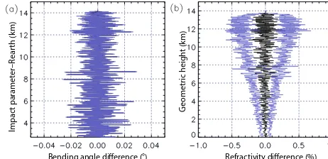
Figure 5a and b show the absolute bending angle error and fractional refractivity error of the FSI retrieval consid-ering the phase noise combined with the in situ refractivity error. The bending angle error is dominated by the phase er-ror of about 0.02◦ across all altitudes with a standard devi-ation maximum of ∼0.007◦near the receiver height due to the in situ refractivity error. The mean refractivity error due to phase noise in the simulation is less than 0.2 % (Fig. 5b). However, the standard deviation of the refractivity error due to the in situ refractivity error reaches a maximum of∼0.5 % and decreases to∼0.05 % near the surface. However, no sys-tematic bias is introduced by such random in situ measure-ment errors.
The refractivity at the receiver is also used to reduce the refractivity errors in the Abel inverse. Figure 3d shows that only the top∼250 m of the bending angle retrieval are noisy, due to the high sensitivity of both the GO and FSI retrieval to the measurement noise in Doppler or phase near the zero ele-vation. To reduce the propagation of larger refractivity errors at the receiver height to lower levels in the refractivity re-trieval, the noisy bending angle observations (e.g., top 250 m below the receiver height) are replaced with a model esti-mate of bending angle, constrained by the in situ refractivity at the receiver extrapolated exponentially with a scale height of 7 km (Murphy et al., 2015). At high flight altitudes where water vapor is very low (e.g., above 9 km), this assumption is justified and the downward propagation of flight level re-fractivity errors is almost completely removed for both GO and FSI retrievals. Ultimately the retrieval accuracy of the airborne technique at flight level is limited by the Doppler errors in the aircraft position (Muradyan et al., 2010) regard-less of retrieval method.
6 Conclusions and discussions
In this study, a FSI algorithm is developed and successfully applied to simulated airborne GNSS RO (ARO) measure-ments for the first time. The simulation study demonstrates the capability of the FSI method to retrieve the atmospheric
Impac
t par
amet
er
–R
ear
th (k
m)
G
eometr
ic heigh
t (k
m)
Bending angle difference (°) Refractivity difference (%)
Figure 5. (a)Mean (black) and standard deviation of FSI-retrieved bending angle error given 1 % Gaussian refractivity error at the
re-ceiver.(b)Same as(a)but for fractional refractivity error.
vertical structure in the lower moist troposphere where fre-quent multipath occurs.
In the FSI retrieval process, the oblateness correction is applied to transform the original occultation geometry to a local spherical radius of curvature to fulfill the local spher-ical symmetric assumption. Then the non-spherspher-ical trajec-tories of both the ARO receiver and the GPS satellite are projected onto circular trajectories relative to local center of curvature. Additional phase correction terms as a result of projection are then added to the measured phase. Afterward, the occultation phase and amplitude time series are divided into positive and negative elevation angle sections. The sep-aration point at the local horizon can be estimated by ray tracing through the CIRA+Q climatological model and se-lecting the epoch when the impact parameter is maximum at the receiver height. The FSI algorithm is then applied to the amplitude and the modified signal phase as a function of open angle for the new circular GPS–receiver trajectories for each time segment. An end-to-end simulation system is used to test the FSI retrieval using the realistic airborne occulta-tion geometry obtained from the PREDICT field campaign.
oc-culted by the Earth. However, such errors resulting from the open-loop tracking at low SNR are not introduced by the re-trieval process (e.g., the FSI rere-trieval) and are best addressed by improvements in antenna design.
Acknowledgements. Funding for this research was provided by NSF grant AGS 1262041. Jennifer S. Haase was supported by NSF grant AGS 1015904. Special thanks to Sergey Sokolovskiy at UCAR for helping develop the prototype FSI retrieval model. Brian Murphy, Kuo-nung Wang, and James Garrison at Purdue University are thanked for useful discussions over the course of the project. We would also like to acknowledge the continued support of NSF program managers Anjuli S. Bamzai and Eric DeWeaver. ERA-Interim reanalysis profiles were provided by the European Centre for Medium Range Forecasts (ECMWF).
Edited by: I. Moradi
Reviewed by: two anonymous referees
References
Born, M. and Wolf, E.: Principles of Optics, Cambridge University Press, New York, 1999.
Fjeldbo, G. F., Kliore, A. J., and Eshelman, V. R.: The neutral atmo-sphere of Venus as studied with the Mariner V radio occultation experiments, Astron. J., 76, 123–140, 1971.
Fowles, G. R.: Introduction to Modern Optics, Dover Publications, Dover, 1989.
Garrison, J. L., Walker, M., Haase, J. S., Lulich, T., Xie, F., Ventre, B. D., Boehme, M. H., Wilmhoff, B., and Katzberg, S. J.: Devel-opment and testing of the GISMOS instrument, paper presented at IEEE International Geoscience and Remote Sensing Sympo-sium, 23–27 July 2007, Barcelona, Spain, 1–4, 2007.
Gorbunov, M. E.: Canonical transform method for processing radio occultation data in the lower troposphere, Radio Sci., 37, 1076, doi:10.1029/2000RS002592, 2002.
Gorbunov, M. E. and Gurvich, A. S.: Microlab-1 experiment: Mul-tipath effects in the lower troposphere, J. Geophys. Res., 103, 13819–13826, 1998.
Gorbunov, M. E. and Lauritsen, K. B.: Analysis of wave fields by Fourier integral operators and their application for radio oc-cultations, Radio Sci., 39, RS4010, doi:10.1029/2003RS002971, 2004.
Gorbunov, M. E., Sokolovskiy, S. V., and Bengtson, L.: Ad-vanced algorithms of inversion of GPS/MET satellite data and their application to reconstruction of temperature and humidity, Tech. Rep. 211, Max Planck Inst. for Meteorol., Hamburg, Ger-many, 1996.
Haase, J. S., Murphy, B., Muradyan, P., Nievinski, F., Larson, K., Garrison, J. L., and Wang, K.-N.: First results from an airborne gps radio occultation system for atmospheric profiling, Geophys. Res. Lett., 41, 1759–1765, 2014.
Hajj, G. A., Kursinski, E. R., Romans, L. J., Bertiger, W. I., and Leroy, S. S.: A technical description of atmospheric sounding by GPS occultation, J. Atmos. Sol.-Ter. Phy., 64, 451–469, 2002.
Healy, S. B., Haase, J., and Lesne, O.:Letter to the EditorAbel
transform inversion of radio occultation measurements made
with a receiver inside the Earth’s atmosphere, Ann. Geophys., 20, 1253–1256, doi:10.5194/angeo-20-1253-2002, 2002. Jensen, A. S., Lohmann, M. S., Benzon, H.-H., and Nielsen, A. S.:
Full spectrum inversion of radio occultation signals, Radio Sci., 38, 1040, doi:10.1029/2002RS002763, 2003.
Jensen, A. S., Lohmann, M. S., Nielsen, A. S., and Benzon, H.-H.: Geometrical optics phase matching of radio occultation signals, Radio Sci., 39, RS3009, doi:10.1029/2003RS002899, 2004. Kirchengast, G., Hafner, J., and Poetzi, W.: The CIRA86aQ_UoG
model: An extension of the CIRA-86 monthly tables including humidity tables and a Fortran95 global moist air climatology model, IMG/UoG Techn. Rep. for ESA/ESTEC, 8, Eur. Space Agency, Paris, France, 1999.
Kursinski, E. R., Hajj, G. A., Schofield, J. T., and Linfield, R. P.: Observing Earth’s atmosphere with radio occultation measure-ments using the Global Positioning System, J. Geophys. Res., 102, 23429–23465, 1997.
Kursinski, E. R., Hajj, G. A., Leroy, S. S., and Herman, B.: The GPS radio occultation technique, Ter. Atmos. Ocean. Sci., 11, 53–114, 2000.
Montgomery, M. T., Davis, C., Dunkerton, T., Wang, Z., Valden, C., Torn, R., Majumdar, S. J., Zhang, F., Smith, R. K., Bosart, L., Bell, M. M., Haase, J. S., Heymsfield, A., Jensen, J., Campos, T., and Boothe, M. A.: The Pre-Depression Investigation of Cloud-systems in the Tropics (PR EDICT) experiment: Scientific basis, new analysis tools, and some first results, B. Am. Meteorol. Soc., 93, 153–172, 2012.
Muradyan, P., Haase, J. S., Xie, F., Garrison, J. L., Lulich, T., and Voo, J.: GPS/INS navigation precision and its effect on airborne radio occultation retrieval accuracy, GPS Solutions, 15, 207–218, doi:10.1007/s10291-010-0183-7, 2010.
Murphy, B. J., Haase, J. S., Muradyan, P. Garrrison, J. L., and Wang, K.-N.: Airborne GPS radio occultation refractivity profiles ob-served in tropical storm environment, J. Geophys. Res.-Atmos., 120, 1690–1709, doi:10.1002/2014JD022931, 2015.
Sokolovskiy, S. V.: Tracking tropospheric radio occultation signals from low Earth orbit, Radio Sci., 36, 483– 498, 2001.
Syndergaard, S.: Modeling the impact of the Earth’s oblateness on the retrieval of temperature and pressure profiles from limb sounding, J. Atmos. Sol.-Ter. Phy., 60, 171–180, 1998.
Vorobev, V. V. and Krasil’nikova, T. G.: Estimation of the accu-racy of the atmospheric refractive index recovery from Doppler shift measurements at frequencies used in the NAVSTAR system, Phys. Atmos. Ocean, 29, 602–609, 1994.
Wang, K. N.: Signal analysis and radioholographic methods for air-borne radio occultations, Doctoral dissertation, Purdue Univer-sity, Purdue, 149 pp., 2015.
Wang, K. N., Garrison, J. L., Acikoz, U., Haase, J. S., Murphy, B. J., Muradyan, P., and Lulich, T. D.: Open-loop tracking of rising and setting GPS radio occultation signals from an airborne platform: signal model and error analysis, IEEE T. Geosci. Remote, 54, 3967–3984, doi:10.1109/TGRS.2016.2532346, 2016.
Xie, F., Haase, J. S., and Syndergaard, S.: Profiling the atmo-sphere using the airborne gps radio occulation technique: A sensitivity study, IEEE T. Geosci. Remote, 46, 3424–3435, doi:10.1109/tgrs.2008.2004713, 2008.